Estimation of white matter fiber parameters from compressed multiresolution diffusion MRI using sparse Bayesian learning

Estimation of White Matter Fiber Parameters from

Compressed Multiresolution Diffusion MRI using

Sparse Bayesian Learning

Pramod Kumar Pisharadya,_{, Stamatios N Sotiropoulos}b_{, Julio M}

Duarte-Carvajalinoa_{, Guillermo Sapiro}c,d_{, Christophe Lenglet}a

a_{CMRR, Radiology, University of Minnesota, Minneapolis, Minnesota, USA} b_{FMRIB, John Radcliffe Hospital, University of Oxford, Headington, UK} c_{Electrical and Computer Engineering, Duke University, Durham, North Carolina, USA}

d_{Biomedical Engineering and Computer Science, Duke University, Durham, North}

Carolina, USA

Abstract

We present a sparse Bayesian unmixing algorithmBusineX:BayesianUnmixing forSparseInference-basedEstimation of Fiber Crossings (X), for estimation of white matter fiber parameters from compressed (under-sampled) diffusion MRI

(dMRI) data. BusineX combines compressive sensing with linear unmixing and

introduces sparsity to the previously proposed multiresolution data fusion

al-gorithm RubiX, resulting in a method for improved reconstruction, especially

from data with lower number of diffusion gradients. We formulate the

estima-tion of fiber parameters as a sparse signal recovery problem and propose a linear

unmixing framework with sparse Bayesian learning for the recovery of sparse

signals, the fiber orientations and volume fractions. The data is modeled using

a parametric spherical deconvolution approach and represented using a

dictio-nary created with the exponential decay components along different possible

diffusion directions. Volume fractions of fibers along these directions define the

dictionary weights. The proposed sparse inference, which is based on the

dictio-nary representation, considers the sparsity of fiber populations and exploits the

spatial redundancy in data representation, thereby facilitating inference from

under-sampled q-space. The algorithm improves parameter estimation from

dMRI through data-dependent local learning of hyperparameters, at each voxel

and for each possible fiber orientation, that moderate the strength of priors

gov-erning the parameter variances. Experimental results on synthetic and in-vivo

data show improved accuracy with a lower uncertainty in fiber parameter

esti-mates. BusineX resolves a higher number of second and third fiber crossings.

For under-sampled data, the algorithm is also shown to produce more reliable

estimates.

Keywords: Sparse Bayesian learning, compressive sensing, linear unmixing ,

diffusion MRI, fiber orientation, sparse signal recovery

1. Introduction

1.1. White Matter Parameter Estimation

Multi-compartment models are used to represent the diffusion MR signal

from the brain white matter and to estimate microstructure features of the

im-aged tissue (Behrens et al., 2003; Panagiotaki et al., 2012; Daducci et al., 2015).

Estimation of orientations and volume fractions of anisotropic compartments in

these models helps infer the white matter fiber anatomy (Behrens et al., 2007).

Accurate estimation of these parameters is challenged by the relatively limited

spatial resolution of diffusion MRI (dMRI) data, which may lead to increased

partial volume artifacts. Advances in magnetic field strength have significantly

improved spatial resolution (Vu et al., 2015), although it may lead to increased

noise and scanning time. One effective way to mitigate the effects of noise is the

multiresolution data fusion approach introduced in RubiX (Sotiropoulos et al.,

2013), which combines high SNR characteristics of low resolution (LR) data with

high spatial specificity of high resolution (HR) data. It allows combining

im-ages with different diffusion contrast at different spatial resolutions and finding

the right trade-off between SNR and resolution. This method was further

ex-tended recently for fusion of data acquired at different magnetic field strengths,

combining the benefits of high spatial and angular resolutions (k / q-space

recent developments in compressive sensing (Ji et al., 2009; Otazo et al., 2015;

Paquette et al., 2015; Duarte-Carvajalino et al., 2014; Michael Lustig and Pauly,

2007; Seeger et al., 2010; Ramirez Manzanares et al., 2007) are effective ways to

deal with the increased scan time, which result in fewer measurements (diffusion

gradients) within a voxel.

Prior efforts in estimation of white matter fiber parameters include both

parametric approaches (Tuch et al., 2002; Behrens et al., 2003; Anderson, 2005;

Kaden et al., 2007; Sotiropoulos et al., 2008, 2013; Coupe et al., 2013;

Scher-rer et al., 2016) and non-parametric approaches (Tournier et al., 2004, 2007;

Ozarslan et al., 2006; Dell’Acqua et al., 2007; Aganj et al., 2010). These

meth-ods exploit multiple diffusion measurements with a large number of diffusion

gradients. Considering the fact that the number of crossing fiber bundles within

a voxel is limited, we propose a novel sparse signal recovery algorithm for

im-proved inference from data with under-sampled q-space (i.e., data acquired with

lower number of diffusion encoding directions). We introduce sparsity based

rep-resentation and inference into the data fusion approach of RubiX, combining the

benefits of regularized noise and reduced scan time.

1.2. Compressive Sensing and Sparse Bayesian Learning

Compressive sensing approaches exploit the sparsity for optimal

acquisi-tion and recovery of signals (Ji et al., 2009; Michael Lustig and Pauly, 2007).

Compressive sensing is used for reconstruction from accelerated imaging

tech-niques across different MRI modalities; in structural MRI (Otazo et al., 2015;

Michael Lustig and Pauly, 2007; Seeger, 2010; Seeger et al., 2010), functional

MRI (Zong et al., 2014), and dMRI (Duarte-Carvajalino et al., 2014; Ramirez

Man-zanares et al., 2007; Rathi et al., 2011; Tristan-Vega A, 2011; Aranda et al.,

2015). A comparison of sampling strategies and sparsifying transforms to

im-prove compressive sensing in diffusion spectrum imaging pointed out the

impor-tance of joint optimization of the sampling scheme and the sparsifying transform

(Paquette et al., 2015).

2001) using automatic relevance determination (ARD) (MacKay, 1994) provides

a framework for obtaining sparse solutions to regression and classification

prob-lems. The sparsity of parameters is enforced by selection of appropriate prior

probability distributions for the parameters to be estimated. Relevance

learn-ing is done in SBL by uslearn-ing a mixture of zero-mean Gaussian distributions with

individual hyperparameters for variance prior distributions. The

hyperparam-eters associated independently with every weight moderate the strength of the

prior and govern the variances of the Gaussian scale mixture, adapting to the

data. Considering the success of SBL for sparse signal recovery in fields such

as computer vision and machine learning (Wright et al., 2010), in this work we

use SBL for the recovery of sparse fiber parameters from dMRI.

1.3. Linear Unmixing

Data sample vectors are assumed to be composed of a mix ofendmembersin linear unmixing algorithms (Dobigeon et al., 2008). Linear unmixing algorithms

estimate both the number of endmembers and their individual contributions.

These algorithms are mostly used in the unmixing of component spectra of

hyperspectral imagery in remote sensing signal processing (Dobigeon et al., 2008;

Bioucas-Dias et al., 2012; Tang et al., 2015; Iordache et al., 2011; Pardo and

Sapiro, 2001; Castrodad et al., 2011).

In this work, we consider the multiple anisotropic components

(correspond-ing to fibers) and the s(correspond-ingle isotropic component in the diffusion model as the

endmembers in unmixing problem, and recover these endmembers using an

SBL based linear unmixing approach. Previous study (Daducci et al., 2014b)

has shown that l1 norm minimization based approaches for promoting

spar-sity, which are widely used in spherical deconvolution based methods, have the

drawback of inconsistency with the sum-to-one constraint (i.e., the physical

constraint that the volume fractions of anisotropic and isotropic compartments

within a voxel sum to unity) (Panagiotaki et al., 2012). They addressed the issue

using a constrained formulation between the data and a sparsity prior bounding

demonstrate that sparse Bayesian learning within a linear unmixing framework

is another way to address the sum-to-one and non-negativity (volume fractions

≥0) constraints, simultaneously promoting sparsity. The approach in SBL is

typically much sparser as it is based on the notion of setting weights to zero

(rather than constraining them to small values), and as it offers probabilistic

predictions without the need to set additional regularization parameters

(Tip-ping and Faul, 2002).

1.4. Proposed Method: Bayesian Unmixing for Sparse Inference-based

Estima-tion of Fiber Crossings (BusineX)

The above mentioned works on compressive sensing in dMRI utilized

basis-based transforms and exploited the sparsity in the basis representation. Our

approach in BusineX is different in several aspects. A major difference is the

Bayesian linear unmixing formulation with SBL based relevance learning. The

unmixing formulation makes the Bayesian inference hard, but it helps in

re-covering fiber parameters with better accuracy, especially when the number of

diffusion measurements are reduced. The SBL framework identifies relevant

fiber orientations by enforcing sparsity, and it further enhances accuracy in

estimation of multi-fiber volume fractions and orientations.

ARD has been used for data-adaptive estimation of fiber parameters (Behrens

et al., 2007), avoiding data unsupported model complexities. The relevance

learning in the proposed approach, which explicitly models sparsity, enhances

the relevance determination by tuning the variance prior hyperparameters

in-dividually and independently for each possible fiber orientation. The

non-negativity and sum-to-one constraints, which make the sparse representation

and inference challenging, are addressed using the linear unmixing framework.

The proposed BusineX algorithm exploits the spatial redundancy in data

rep-resentation, and it improves the estimation of fiber parameters. The number

of fibers that best fit the observed data is estimated by the automatic

detec-tion of number of endmembers using a reversible jump Markov chain Monte

case, the proposed algorithm is shown to produce reliable estimates from data

under-sampled in q-space, by a factor of up to four.

The results from a preliminary version of the proposed framework with linear

unmixing (without relevance learning using SBL) are presented in our prior work

(Pisharady et al., 2015). In this paper we extend the framework by introducing

SBL based relevance learning. The paper also presents detailed experimental

results and analysis, including comparisons of estimated fiber volume fractions

in addition to the fiber orientations and diffusivity.

2. Methods

This section details the proposed BusineX algorithm. The dictionary

repre-sentation of the HR data using compartment model (ball & stick) is described

in Subsection 2.1. The representation of LR data using a spatial partial

vol-ume model is briefly discussed in Subsection 2.2. The sparse Bayesian learning

approach and sparsity based linear unmixing algorithm are described in

Sub-sections 2.3 and 2.4 respectively. Subsection 2.5 explains the MCMC sampling

procedure.

2.1. Dictionary Representation of High Resolution Data

The HR data is represented using a dictionary containing exponential decay

component vectors in the compartment model of diffusion. The measured dMRI

signal at each HR voxel is first modeled using the ball & stick (1) model (Behrens

et al., 2003; Panagiotaki et al., 2012),

S_HRk =S0_HR

" 1−

N

X

n=1 fn

!

e−bkd₊

N

X

n=1

fne−bkd(g

T kvn)2

#

(1)

where,

S_HRk is the signal at HR voxel after application ofkthdiffusion-sensitizing gradient with directiongk and b-valuebk,

S0

HR is the HR signal without diffusion gradient applied,

fn is the volume fraction of anisotropic compartment with orientationvn, and

The measured signal at an HR voxel is the sum of the attenuation signal and

measurement noise (2),

y_HRk =S

k HR

S0

HR

+η_HRk . (2)

Based on (1) and (2), the measured signal along all K diffusion-sensitizing

directions can be written in adictionary form (3) as

yHR= 

   

e−b1d _e−b1d(gT1v1)2 _{. . . e}−b1d(gT1vN)2 ..

. ... . .. ...

e−bKd _e−bKd(gKTv1)2 _{. . . e}−bKd(gTKvN)2

             f0 f1 .. . fN        

+ηHR, (3)

where

f0= 1−

N

X

n=1 fn

!

, fn≥0.

Hence,

yHR= Ef +ηHR. (4)

In Equation (4),Erepresents the local dictionary matrix (5) for the HR diffusion data andf is the sparse vector representation of the HR data in this dictionary

E. The non-zero entries in f define the number and volume fractions of fibers (sticks) in a voxel.

E=     

e−b1d _e−b1d(gT1v1)2 _{. . . e}−b1d(gT1vN)2 ..

. ... . .. ...

e−bKd _e−bKd(gTKv1)2 _{. . . e}−bKd(gKTvN)2

     . (5)

The possible orientations of anisotropic components in the dictionary (second

column onwards) are pre-specified and formed using a 5th _{order icosahedral}

tessellation of the sphere with 10242 points. The estimated orientation is

ap-proximated to the nearest pre-specified orientation during the dictionary update

process.

With the above dictionary formulation, the problem of finding the number of

sparse vectorf. The estimation of the sparse vectorf is detailed in Subsections 2.3 and 2.4. Another unknown parameter in the model, the apparent diffusivity

d, is estimated through the Bayesian inference that maximizes the joint posterior

probability of the HR and LR data, as per the multiresolution graphical model

in RubiX (Sotiropoulos et al., 2013), as detailed in Appendix A. The partial

volume model used to represent the LR data is discussed in the next Subsection

(Subsection 2.2).

2.2. Partial Volume Representation of Low Resolution Data

The significance of LR data is its high SNR, which is useful for regularizing

the noise in HR data, as in the RubiX framework (Sotiropoulos et al., 2013). In

the RubiX framework, the LR data and HR data are collected from the same

subject through two scans at different spatial resolutions (voxel sizes). The two

datasets are aligned (if necessary) using rigid body transformations. Once the

data is aligned, the LR data can be represented using corresponding HR data

(data that correspond to the same physical location, but at a different spatial

resolution grid), with a partial volume model (Sotiropoulos et al., 2013). The

model calculates attenuation signal at an LR voxel as a linear combination of

the signals at overlappingM HR voxels (6).

Sk LR

S0

LR

=

M

X

m=1 wm

Skm HR

S0m HR

, wm=e

−krm−r0k2

γ2 _{. (6)}

The HR signal contributes to the LR signal via a discretized Gaussian distance

weighing function (DWF) with weightswmgiven by the normalized Euclidean

distance between the DWF center r0 at LR voxel and the spatial position of

each HR voxel rm, and the unknown standard deviation of the DWF, γ. γ

is same forM HR voxels overlapped by an LR voxel, but can be different for

different LR voxels.

2.3. Hierarchical Bayesian Inference and Sparse Bayesian Learning

The volume fractions and fiber orientations are estimated using a

sparse Bayesian inference dealing with constraints (Araki et al., 2009; Tipping,

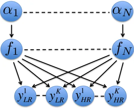
2001). A hierarchical Bayesian framework (Fig. 1) is utilized for the sparse

inference. In Bayesian inference, prior probability distributions, namelypriors,

are defined for constraining the parameters to be estimated (Jaynes, 1968). In

SBL a mixture of zero-mean Gaussian distributions with individual

hyperpa-rameters controlling the variances is used as the prior on the parameter to be

estimated (volume fractions here). Gamma distributions are used as

hyperpri-ors, which form the priors over the hyperparameters. The mixture of Gaussians

with hyperparameters associated independently with every weight was shown

equivalent to using a product of Student-t priors, once the hyperparameters are

integrated out (Tipping, 2001). This hierarchical formulation leads to a sparse

solution.

Figure 1: The hierarchical Bayesian network used in BusineX.yk

LRandyHRk are the measured signals along diffusion gradient directionk, at LR and HR voxels respectively.fnis the n-th

component of the anisotropic volume fractions vector andαn is the hyper-parameter in the

prior distribution offn. The influence of the parameters on LR data is through the spatial

partial volume model (6).

Mathematically the prior over volume fractions is given by,

p(f|α) =

N

Y

n=1

where the hyper-parameter αn controls the variance of individual Gaussians.

The update procedure forαi (detailed in Subsection 2.4) is such that many of

theαare pushed to higher values, adapting to the data. The variance 1/α of

the corresponding Gaussians are pushed towards zero which forces the

corre-sponding weights to be zero (or negligibly small), leading to a sparse solution.

The proposed sparse approach and independent tuning of the

hyperparam-eters for each voxel and for each possible fiber orientation promote adaptation

of the estimated number of fibers to the data. Thus the complexity of fiber

patterns (single fiber vs. multiple fibers) at each voxel is decided better by the

data (refer to Section 4.1 for a discussion).

2.4. Sparsity based Bayesian Linear Unmixing Inference

Finding the volume fractions f in (4) with a large number of possible fiber orientations (N) is an ill-posed problem. We introduce sparsity in the dictionary

and estimation process, to propose an efficient algorithm for volume fraction and

fiber orientation estimations. The non-negativity and sum-to-one constraints of

volume fractions make the sparse representation and inference especially

diffi-cult. We fix the sparsity level (the number of fibers, which is the same as the

number of non-zero anisotropic components) to a small numbern0 (n0<< N).

The problem is then formulated as a linear unmixing inference where the

diffu-sion signals correspond to a mixture of the dictionary components with positive

weights f. We follow a semi-supervised hierarchical Bayesian linear unmixing approach (Dobigeon et al., 2008) for sparsity-based inference of fibers. The

method is semi-supervised because the dictionary is known for a given

diffusiv-ity, gradient directions, b-values, and possible fiber orientations, but we don’t

know the values of diffusivity, fiber orientations, or the volume fractions within

each compartment.

Assuming Gaussian noise1 the likelihood function of the HR data can be

1_{We implemented Rician noise model (Henkelman, 1985) as well, which provided identical}

expressed as (8)

p yHR|f, α, σ2

=

₁

2πσ2

K2 e−

kyHR−Efk2₂

2σ2 _{, (8)}

where σ2 corresponds to the variance of the error in representation of yHR

using dictionary E and volume fractions f. Let f+ _{= [f}

1, . . . , fn0]

T _{be the}

volume fractions withn0 non-zero anisotropic components, thenf+ belongs to

a simplexS (9),

S= (

f+|fn>0,∀n= 1, . . . , n0, n0

X

n=1 fn≤1

)

. (9)

Once the prior and likelihood are defined, Bayesian inference proceeds by

calculating the posterior using Bayes’ rule. The generative model of RubiX is

adapted here with a novel inference algorithm for the volume fractions and fiber

orientations. The proposed algorithm introduces an additional layer of adaption

to the data adaptive ARD framework, to enhance the automatic detection of

the number of fibers, by tuning the volume fraction variance for each possible

fiber orientation and by explicitly modeling sparsity to improve the relevance

determination.

The volume fractions posterior is given by (10) (Tipping, 2001)

p f+, α, σ2|yHR

=p yHR|f

+_{, α, σ}2

p f+_{, α, σ}2

p(yHR)

. (10)

We cannot compute (10) as the normalizing integral (11) cannot be computed

analytically.

p(yHR) =

Z

p yHR|f+, α, σ2

p f+, α, σ2df+dα dσ2. (11)

Instead the posterior (10) is decomposed as

p f+, α, σ2|yHR=p f+|yHR, α, σ2p α, σ2|yHR, (12)

where

p f+|yHR, α, σ2=

p yHR|f+, σ2p(f+|α)

p(yHR|α, σ2)

. (13)

We can compute (13) as its normalizing integral (14) is a convolution of

Gaus-sians (Tipping, 2001),

p yHR|α, σ2

=

Z

p yHR|f+, σ2

p f+|α

df+. (14)

We now introduce the linear unmixing framework to the sparse inference.

Blind unmixing under positivity constraints was introduced by Moussaoui et

al. (Moussaoui et al., 2006). Dobigeon et al. (Dobigeon et al., 2008) further

extended this by including the sum-to-one constraint, attempting to resolve the

scale indeterminacy inherent in blind source separation problems. We

intro-duce these linear unmixing constraints to the posterior computation in (13), to

propose sparsity based linear unmixing inference (15),

p f+|yHR, α, σ2

∼e−(f+−µf) T

Λ−_f1(f+−µf)1

S(f+), (15)

where

Λf =

h

σ−2 E_n+₀−e0uT

T

E_n+₀−e0uT

+Ai

−1

, (16)

and

µf =σ−2Λf En+0−e0u

TT

(yHR−e0), (17)

withuis a 1 xn0vector, [1, . . . ,1]T, andA=diag(α0, α1, ..., αN). En+0contains

the columns of E that correspond to n0 non-zero coefficients in f+ _(effective

dictionary) and e0 is the column corresponding to the isotropic compartment

(ball in the HR model). 1S(f+) in (15) is 1 iff+∈S and 0 otherwise.

Each hyper-parameter αn in A are updated iteratively (Tipping, 2001) as

per (18),

αnew_n =γn/µ2n, (18)

whereγn= 1−αn∗Λnn, and Λnn is thenthdiagonal element of the posterior

volume fractions covariance (16). The noise varianceσ2is updated as per (19),

(σ2)new=k(yHR−e0)−(E

+

n0−e0uT)µfk2

K−P

nγn

. (19)

The priors we used for volume fractions are a mixture of Gaussians with

We followed the rest of the parameter priors and the inference procedure2, in-cluding the estimation of diffusivityd, as in RubiX (Sotiropoulos et al., 2013).

The priors used forS0andσare unconditional and non-informative (uniform). Conditional priors are used for orientation and diffusivity and are defined as

a mixture of Watson distributions with non-informative hyper-parameter for

orientation and normal distribution with informative hyper-parameter for

dif-fusivity.

2.5. Hybrid Metropolis-Within, Reversible Jump Gibbs Sampler for Detecting

the Number of Fibers

The generation of samples according to (15-17) is accomplished using a Gibbs

sampler (Algorithm 1). It proceeds by repeated application of (18) and (19) and

the corresponding updates of posterior statistics Λf andµf from (16) and (17).

Each column in the effective dictionary E+_n0 can be switched at random with another to test a different fiber orientation.

In order to find the number of fibers that best fits the data automatically we

used a metropolis-within reversible jump Gibbs sampler (Dobigeon et al., 2008)

whichkills orgenerates fibers as per the death and birth probabilities (Denison

et al., 2002), respectively (Algorithm 1). The following 3 cases can occur in

each iteration:

• CASE 1 - Add a new fiber through BIRTH move: The volume fraction

of the new fiber is drawn from a Beta distribution, Be(1, n0). The other

anisotropic volume fractions are scaled so that anisotropic and isotropic

volume fractions sum to one.

• CASE 2 - Remove a fiber throughDEATH move: The remaining anisotropic

volume fractions are scaled so that anisotropic and isotropic volume

frac-tions sum to one.

Algorithm 1Hybrid Metropolis-Within Reversible Jump Gibbs Sampler 1: procedureInitialization

2: InitializeE; %dictionary, using ball&stick model f itting(1) 3: Initializef+; %volume f ractions, using ball&stick model f itting(1) 4: Initialize prior probabilities;

5: Initializeα+_;

6: end procedure

7: procedure_Iterations % we used 1,500 iterations 8: fori=1 to # iterations do

9: Calculate Λf andµf; %posterior covariance&mean, (16) & (17)

10: Updateα+; %variance of volume f ractions prior(18) 11: Updateσ2; %noise variance (19)

12: Switch(p) %p is random[0−1], cases p≤1/3, 1/3< p≤2/3, p >2/3 13: CASE 1: ProposeBIRTH move,n0=n0+ 1;

14: CASE 2: ProposeDEATH move,n0=n0−1;

15: CASE 3: ProposeSWITCH move,n0=n0;

16: End

17: Accept / RejectBIRTH / DEATH / SWITCH move;

18: propose newf+; %new volume f ractions proposal

19: end for

• CASE 3 - Maintain the number of fibers throughSWITCH move: Neither

a fiber is added nor removed. The inference is proceeded by switching the

fiber orientations, columns in the effective dictionaryE_n+₀ .

In our experiments, we limited3 _{the maximum number of anisotropic}

compo-nents (the number of fibers), nmax

0 to 3. No BIRTH move is allowed when

n0=nmax0 and noDEATH move is allowed whenn0= 1. In all iterations, all

possible cases (from the above 3 cases) are kept equally likely, i.e. probability

of 1/3 when all the 3 cases are possible and 1/2 when only 2 cases are possible.

The update in the number of fibers is accepted or rejected based on the

move acceptance probability. The acceptance probability for aBIRTH moveρb

is given byρb=min{1, Ab}, whereAb is the acceptance ratio. The acceptance

probability for aDEATH moveρdis given byρd=min{1, Ad}, whereAdis the

rejection ratio (refer Appendix B for the derivation of Ab and Ad). SWITCH

moves are accepted or rejected using Metropolis sampling criterion.

3. Experiments and Results

We conducted experiments using 2 sets of synthetic data and one set of

in-vivo data. The datasets and the results are detailed in this section.

3.1. Synthetic Data from HARDI Reconstruction Challenge

The first synthetic data we used is simulated from the 2 structured field

phantoms used to evaluate algorithms in the HARDI reconstruction challenge

organized as part of theISBI 2012 conference (Daducci et al., 2014a). We used

this challenging dataset with complex fiber configurations to test the general

performance of the algorithm and to compare it with other existing methods.

We used 50 diffusion gradients to simulate the data, using a multi-Tensor model.

3_{We limited the maximum number of fibersn}max

0 to 3 to have a reasonable convergence time, and since more than 3 fibers is not expected. The algorithm is generic with respect to

nmax

Daducciet al. (Daducci et al., 2014a) reported the results of the challenge and

compared 20 algorithms used for recovering the intra-voxel fiber structures.

Here we compare the performance of BusineX using these reported results.

There are 2 phantoms in the structured field dataset, a simple one (the

dataset released with the challenge announcement, the training set, hereafter

called ISBI dataset-1) and a complex one (the dataset used to evaluate

algo-rithms to decide the winner, the testing set, hereafter called ISBI dataset-2).

Both phantoms had a size of 16×16×5 voxels. We copied the 5th slice of the

phantom and added it as an additional slice to generate the dMRI data with

an image size 16×16×6, using the simulation algorithm the challenge

organiz-ers released (http://hardi.epfl.ch/static/events/2012_ISBI/download.

html#testingdata). We added the 6th slice as we need to simulate the LR dataset with half the resolution with an image size 8×8×3, which we did by

down-sampling the HR data to LR image size (averaging the signals at groups

of 2×2×2 HR voxels). We report the average results from all the voxels (6

slices) making the comparisons fair with the average results (5 slices) reported

previously (Daducci et al., 2014a). The HR data is simulated at an SNR 10

(with Rician noise) (Daducci et al., 2014a). A factor of 8/√2 is maintained in

the ratio of SNR of LR to that of HR signal (Sotiropoulos et al., 2013).

Fig. 2 shows a visualization of the orientations and the sum of anisotropic

volume fractions (upper panels) estimated from ISBI dataset-1 (SNR=10), which

has the same sum of volume fractions (unity) at every voxel. The histograms of

corresponding sum of anisotropic volume fractions (lower left panel) and

orien-tation error (lower right panel) for all the voxels show the improved estimations

in BusineX.

We further evaluated and compared the performance of BusineX using 2

criteria, the correct assessment of the number of fiber populations expressed

withsuccess rateand the error in orientation estimation expressed withangular

precision (Daducci et al., 2014a). These measures are reported for the testing

Figure 2: Comparison showing volume fraction and orientation estimations from the ISBI

dataset-1. The SNR of the data is 10. Color coded orientation estimates from BusineX

(upper left panel) and RubiX (upper right panel) are shown with the corresponding sum of

anisotropic volume fractions in the background. Lower panels show the normalized histograms

of sum of anisotropic volume fractions (left) and orientation error (right) for both cases, for all

the 6 slices. The comparisons show the improved volume fraction and orientation estimations

3.1.1. Success Rate and Angular Precision

The success rate and angular precision is calculated as below (20 and 21)

(Daducci et al., 2014a).

Success Rate(SR) =

1−|Mtrue−Mestimated| Mtrue

× 100, (20)

whereMtrue andMestimated are, respectively, the true and estimated number of

fiber compartments inside a voxel.

Angular P recision(AP) = 180

π arccos(|dtrue·destimated|), (21)

where dtrue and destimated are a pair of true and estimated fiber orientation

vectors in a voxel.

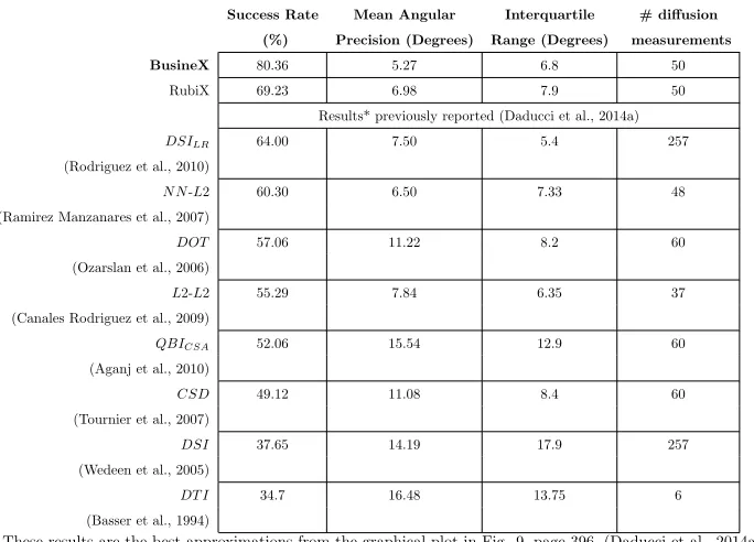
The reported results are the mean SR and AP across all voxels and fibers

(Table 1). The better performance of BusineX is evident in these results. In

particular, for dataset-2 (the dataset used to evaluate algorithms to decide the

winner of the challenge), BusineX provided an SR of 80.36%, 11.13% better

than RubiX (69.23%) and 16.36% better than the algorithm reported as top

in SR (64%) (Rodriguez et al., 2010), in the comparison provided in (Daducci

et al., 2014a) (Refer Fig. 9, page 396). This shows the benefit of BusineX in

detecting fibers more accurately, which is made possible through the explicit

calculation of volume fractions posterior probability (15), as detailed in Section

2.4. Table 1 also reports the interquartile range representing the dispersion in

AP and also the number of diffusion measurements used by each method.

The results reported in Table 1 are obtained using the uncorrected SNRs

from (Daducci et al., 2014a). The SNR corrected for the variable echo-time

(TE) is 24.3 in our case (b-values 1500, see Table II in (Daducci et al., 2014a)).

We also did experiments with a corrected SNR of 24.3 (instead of 10). The

corresponding SR and AP are 82.99% and 4.88 degrees respectively.

In order to study whether the estimated fiber populations are close enough to

the real ones, we calculated the SR using thetolerance cone approach (Daducci

Table 1: Mean Success Rate and Angular Precision - ISBI dataset-2

Success Rate Mean Angular Interquartile # diffusion

(%) Precision (Degrees) Range (Degrees) measurements

BusineX 80.36 5.27 6.8 50

RubiX 69.23 6.98 7.9 50 Results* previously reported (Daducci et al., 2014a)

DSILR 64.00 7.50 5.4 257

(Rodriguez et al., 2010)

N N-L2 60.30 6.50 7.33 48

(Ramirez Manzanares et al., 2007)

DOT 57.06 11.22 8.2 60 (Ozarslan et al., 2006)

L2-L2 55.29 7.84 6.35 37 (Canales Rodriguez et al., 2009)

QBICSA 52.06 15.54 12.9 60

(Aganj et al., 2010)

CSD 49.12 11.08 8.4 60 (Tournier et al., 2007)

DSI 37.65 14.19 17.9 257 (Wedeen et al., 2005)

DT I 34.7 16.48 13.75 6 (Basser et al., 1994)

* These results are the best approximations from the graphical plot in Fig. 9, page 396, (Daducci et al., 2014a).

DT I- diffusion tensor imaging,DSI- diffusion spectrum imaging,DSILR- DSI Lucy-Richardson,DOT- diffusion

orientation falls within a tolerance cone of 20◦around the real fiber population.

This measure, which is reported as SR6 (Daducci et al., 2014a) is 70.95% for

BusineX and 63.86% for RubiX.

3.2. Synthetic Data Simulated using Camino

To study the effect of under-sampling and to have uniform ground truth

values for volume fractions, we simulated a second synthetic dataset using the

Camino toolbox (Cook et al., 2006). A Tensor-Cylinder-Sphere model is used

to simulate single and crossing fiber structures (with 2 and 3 fibers) with image

size 10×10×2 (LR) and 20×20×4 (HR), at different under-sampling factors.

The diffusivity value used to simulate the data is 1.7 x 10−9m2_{/s. To make}

the fiber pattern in the image continuously varying, the orientation of fibers at

each HR voxel is selected such that it varies across each dimension by 1 degree

/ voxel. A minimum crossing angle of 45 degrees is maintained in this case.

Diffusion signals are simulated along 200 uniformly distributed directions, with

a b-value of 1500s/mm2. The noise free LR signal is created by down-sampling the HR data to LR image size (averaging the signals at groups of 2×2×2 HR

voxels). Rician noise is added to both LR and HR images by adding zero-mean

Gaussian signal in quadrature. A factor of 8/√2 is maintained in the ratio of

SNR of LR to that of HR signal (lower noise in LR data) (Sotiropoulos et al.,

2013). We simulated HR data with two SNRs, 15 and 25. Under-sampling of

diffusion directions is done by a factor of up to four to simulate acceleration in

image acquisition.

The algorithm performance is compared with the ball & stick model applied

to the HR dataset (usingBedpostX tool (Behrens et al., 2007) in FSL) and

Ru-biX (Sotiropoulos et al., 2013) applied to HR and LR datasets. Both RuRu-biX and

BusineX are applied to HR and LR datasets, with the first 100 measurements

forming theno-accelerationdata. This is done in order to approximately match

the acquisition time, making the comparisons fair (as BedpostX uses data at

only HR resolution). The 100 measurements are under-sampled again up to

Caruyeret al. (Caruyer et al., 2011) for under-sampling, which makes any first

N samples isotropic.

3.2.1. Fiber Orientation Estimation

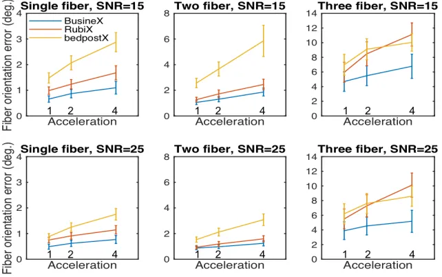
Fig. 3 shows the mean error and standard deviation in fiber orientation

estimation, and the variations with acceleration, for 1, 2, and 3 fiber cases,

with SNR 15 and 25. On comparison, BusineX provided better estimation

accuracy, at a slightly lower uncertainty. The variation in estimation error with

acceleration is lower in BusineX.

Figure 3: Comparison of fiber orientation estimation error (mean across 1600 voxels) and

its variation with acceleration factor (under-sampling in number of diffusion measurements).

Three data points with no under-sampling (1), under-sampling by a factor of 50% (2) and

under-sampling by a factor of 75% (4) are shown. Y-axis represents mean error across voxels

and across fibers in 2 and 3 fiber cases. The error bars shown represent the standard deviation

in estimation (scaled by 50% for all the methods, for better visualization), representing the

3.2.2. Fiber Volume Fraction Estimation

Fig. 4 presents the histogram results of volume fraction estimation in the 2

fiber case with SNR 15. The true value of both fiber 1 and 2 volume fractions

is 0.3. The comparisons show the improved volume fraction estimation in both

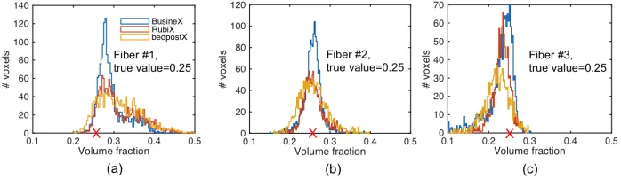
first and second fiber cases. A similar comparison in the 3 fiber case is shown

in Fig. 5, in which each fiber has equal volume fractions of 0.25.

Figure 4: Comparison of volume fraction estimation in the 2 fibers case (SNR=15,

no-acceleration). (a) & (b) are histograms of estimated volume fractions of fiber #1 & # 2

respectively. Each of the fibers have a true volume fraction of 0.30, marked with red cross on

the x-axis. The total number of voxels having a volume fraction of 0.3 is 1600.

Figure 5: Comparison of volume fraction estimation in the 3 fibers case (SNR=15,

no-acceleration). (a)-(c) are histograms of estimated volume fractions of fiber #1, #2, & #3

respectively. Each of the fibers have a true volume fraction of 0.25, marked with red cross on

the x-axis. The total number of voxels having a volume fraction of 0.25 is 1600.

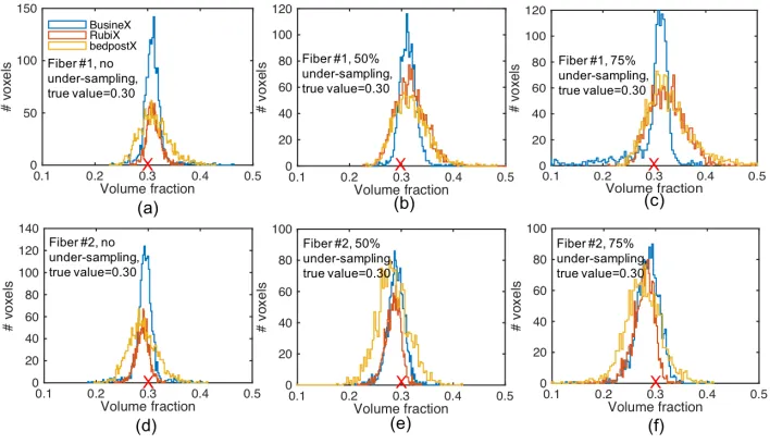
acceleration. Fig. 6 shows a comparison under different accelerations

(under-sampling factors) in 2 fibers case with SNR 15.

Figure 6: Comparison of volume fraction estimation of fiber 1 (row 1) and fiber 2 (row 2) at

different under-sampling factors. Left column shows the case with no under-sampling, middle

column shows the case with 50% under-sampling, and the right column shows the case with

75% under-sampling. Each of the fibers have a true volume fraction of 0.30, marked with red

cross on the x-axis. The total number of voxels having a volume fraction of 0.3 is 1600. The

SNR of the data is 15.

3.2.3. Diffusivity Estimation

We used a diffusivity value of 1.7 x 10−9_m2_{/sfor the data simulation using}

Camino. The estimated mean diffusivity (mean of the diffusivity across 1600

voxels) is 1.6868 x 10−9m2_{/s with a variance 1.02 x 10}−21_{. RubiX provided}

identical results: mean diffusivity of 1.6813 x 10−9m2_{/s with a variance 1.14}

x 10−21. BedpostX provided slightly lower accuracy in diffusivity estimation:

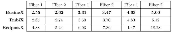
3.2.4. Estimation Uncertainty

Table 2 provides mean span of 95% cones of uncertainty, which is a measure

of the width of estimated distributions, representing the uncertainty in

esti-mation. The estimation uncertainty in BusineX is slightly better than that in

RubiX, and the estimation uncertainty in BedpostX is approximately two times

that in BusineX.

Table 2: Comparison of estimation uncertainties - Mean span of 95% cones of orientation

uncertainty (in degrees)

No under-sampling 50% under-sampling 75% under-sampling

Fiber 1 Fiber 2 Fiber 1 Fiber 2 Fiber 1 Fiber 2

BusineX 2.55 2.62 3.31 3.47 4.63 5.00

RubiX 2.65 2.74 3.50 3.70 4.80 5.12

BedpostX 4.88 5.24 6.93 7.89 10.7 18.28

3.3. In-vivo Data Acquired using 3T Siemens Prisma Scanner

We acquired in-vivo data from a healthy subject using 3T Siemens Prisma

scanner. For HR acquisitions the acquisition matrix was 140×140×92 voxels

with a resolution of 1.5×1.5×1.5mm3. For LR acquisitions the resolution was reduced to 3×3×3 mm3 for an acquisition matrix size 70×70×46 voxels. Diffusion weighting was applied in 200 evenly spaced directions with a b-value

of 1500 s/mm2_{. Twenty one volumes without diffusion weighting are equally}

interleaved in the dataset.

3.3.1. In-vivo Data Results

We report 4 sets of results from the in-vivo experiments showing, a) the

stability of fiber orientation and volume fraction estimates with acceleration

(Fig. 7),b) improved estimation of orientation and volume fractions (Fig. 8, 9

Fig. 11), andd) improved diffusivity estimation (Fig. 12). We used the

Con-nectome Workbench (Marcus et al., 2011) from the Human ConCon-nectome Project

for visualizing the results4 (Fig. 7-10).

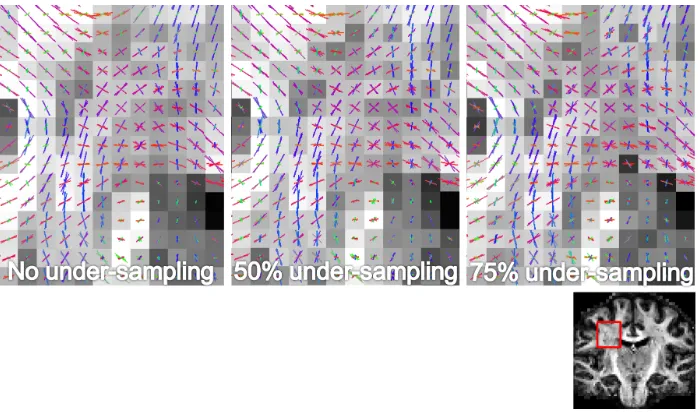
Fig. 7 shows a representative comparison of fiber orientation and sum of

volume fractions estimates at different accelerations (under-sampling factors in

number of diffusion scans). The region shown is the centrum semiovale area,

where commissural fibers (the corpus callosum, CC) and association fibers (the

superior longitudinal fasciculus, SLF) crosses the projection fibers (the

corti-cospinal tract, CST). The comparison shows the robustness of fiber orientation

and volume fraction estimates with acceleration.

We compare our in-vivo results to the reconstructions provided by RubiX

(Sotiropoulos et al., 2013), BedpostX (Behrens et al., 2007), and Constrained

Spherical Deconvolution (CSD) (Tournier et al., 2007). The implementations

of BedpostX available in FSL (Jenkinson et al., 2012a) and CSD available in

MRtrix3 (Tournier et al., 2012) are used for the experiments. The method used

for calculation of the response function is tourneir and for fiber orientation

distribution is csd. The spherical harmonic order (lmax) used is the default

value in MRtrix3 (lmax= 8). The visualization tool in MRtrix (mrview) is used

to visualize the estimated Orientation Distribution Functions (ODFs).

Fig. 8 provides representative comparisons from the centrum semiovale area,

showing improved detection of crossing fibers by BusineX, as compared to

Ru-biX. Fig. 9 compares performance of BusineX with that of RubiX, BedpostX,

and CSD, showing improved estimations of the fibers crossing the pons. The

highlighted regions show improved detection of crossing fibers by BusineX.We

calculated the mean sum of volume fractions of first, second, and third fibers

from the region of interest (ROI) highlighted in red in Fig. 9. BusineX,

Ru-biX, and BedpostX provided values of 0.469, 0.399, and 0.408 respectively. The

4_{The processing in Workbench estimates bingham distributions from the set of estimated}

posterior fiber parameter samples, for each fiber orientation in a voxel which is labeled a

Figure 7: Comparison showing the stability of fiber orientation and volume fraction estimates

with acceleration (under-sampling). Upper panel shows color coded orientation estimates at

the region near the centrum semiovale, highlighted in the coronal view in lower panel. The

background to the orientation estimates is the sum of anisotropic volume fractions. In the

upper panel left column shows the case with no under-sampling, middle column shows the case

Figure 8: Comparison between BusineX and RubiX, showing improved detection of crossing

fibers by BusineX. Panels 2 and 3 show color coded orientation estimates at the region near

right and left centrum semiovale, highlighted in the coronal view in uppermost and lowermost

panels, respectively. The background to the orientation estimates is the sum of anisotropic

volume fractions estimated by each method. The estimation is done from HR and LR datasets

higher mean sum of volume fractions obtained from BusineX may correspond

to improved detection of crossing fibers.

Fig. 10 shows another comparison of the performance of BusineX with

that of RubiX, BedpostX, and CSD, showing improved parameter estimates

near SLF. We also analyzed the performance improvement quantitatively, by

counting the number of second and third fiber crossings in the white matter, as

well as in several specific ROIs. Fig. 11 shows the number of second and third

fiber crossings in the white matter, near the pons in the ROI from Fig. 9, in the

left/right SLF and in the left/right posterior corona radiata (PCR). It can be

noticed that, while RubiX and BedpostX tend to recover fewer second and third

fiber crossings as the under-sampling factor increases, BusineX performs equally

well even with only a quarter of the original diffusion gradients. Lastly we have

shown a map of the estimated mean diffusivity in Fig. 12. By comparison with

DTI, both BusineX and BedpostX provide diffusivity estimates with improved

contrast. Compared to BedpostX, the estimate from BusineX also appears to

be less noisy.

4. Discussion

4.1. Complexity of Fiber Patterns

The use of SBL in BusineX enhances the variance adaptation of fiber volume

fractions to the data, at each voxel and for each possible fiber orientation. This is

made possible by moderating the strength of priors through associated

hyperpa-rameters. In other words, the proposed framework performs relevance learning

by tuning the variance hyperparameters spatially (across voxels) and angularly

(across possible fiber orientations), which is the main novelty of our approach.

Contrary to earlier approaches in fiber parameter estimation, which utilizes a

fixed ARD weight for all voxels and fibers (Behrens et al., 2007; Sotiropoulos

et al., 2013), this variance adaption through relevance determination improves

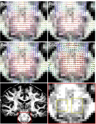
Figure 9: Comparison between BusineX, RubiX, BedpostX and CSD showing improved

de-tection of fibers crossing the pons. Upper and middle panels show color coded orientation

estimates (ODF in the case of CSD) at the pons region highlighted in the coronal view in

lower left panel. The background is the sum of anisotropic volume fractions estimated by

BedpostX for all the methods. A comparison of the areas highlighted in the lower right panel

shows improved detection of CST fibers at the level of the pontine crossing tract. The

estima-tion from BedpostX and CSD is done from the full HR dataset with 200 diffusion direcestima-tions.

The estimation from BusineX and RubiX is done from HR and LR datasets with 100 diffusion

directions per dataset. We use a total of 200 directions in all experiments to approximately

match the acquisition time (LR acquisitions can be done faster than HR). BedpostX and CSD

use only one dataset (HR), whereas BusineX and RubiX use two datasets (HR and LR) with

Figure 10: Comparison between BusineX, RubiX, BedpostX, and CSD showing improved

detection of crossing fibers by BusineX. Upper panels show color coded orientation estimates in

the SLF region highlighted in the sagittal view in lower right panel. Lower left panel shows the

color coded ODF estimated using MRtrix.The background is the sum of anisotropic volume

fractions estimated by BedpostX for all the methods. A comparison of the areas highlighted

in the lower middle panel shows improved detection of association fibers through the SLF.

BusineX resolves the association fibers in both highlighted areas. RubiX and BedpostX do

not resolve all the fibers at the yellow area, and CSD does not resolve all the fibers at the

magneta area. The estimation from BedpostX and CSD is done from the full HR dataset

with 200 diffusion directions. The estimation from BusineX and RubiX is done from HR and

LR datasets with 100 diffusion directions per dataset. We use a total of 200 directions in all

experiments to approximately match the acquisition time (LR acquisitions can be done faster

than HR). BedpostX and CSD use only one dataset (HR), whereas BusineX and RubiX use

Figure 11: Variation in number of second and third fiber crossings (with volume fractions

greater than 5%) in the white matter and in five selected ROIs.

Figure 12: Estimated mean diffusivity maps from BusineX (left), BedpostX (middle), and

the improved performance of BusineX, as illustrated in our simulation as well

as in-vivo results.

Another reason for the possible improvement in detection of crossing fibers

is the automatic tuning of fiber complexity using the hybrid Metropolis-within

reversible jump Gibbs sampler (Section 2.5), which helps fiber complexity

adap-tation by accepting or rejecting addition and deletion of fibers. Also, the

rescal-ing of volume fractions after every addition (BIRTH) and deletion (DEATH) move, as per the non-negativity and sum-to-one constraints, further facilitates

improvement in parameter estimation.

4.2. Local and Spatial Diffusion Models

The proposed algorithm is generic with respect to the local diffusion model

and the corresponding model parameters. The algorithm can be applied to

any model which can represent the data in dictionary form (Section 2.1) . We

chose the ball & stick model to approximate the diffusion signal, but it can

be replaced with more complex models such as a non-monoexponential decay

model to approximate multi-shell data (Jbabdi et al., 2012). In order to support

the flexibility of the proposed method, we used different models for synthetic

data simulation: A Tensor-Cylinder-Sphere model for the Camino dataset and

a Multi-Tensor model for the ISBI HARDI dataset.

To verify our spatial model, the assumption that the attenuation signal at an

LR voxel can be approximated by a weighted linear combination of attenuation

signals at corresponding overlapping HR voxels (6), we calculated the mean

and standard deviation of the root mean square error (RMSE) of estimated LR

attenuation signal from the actual LR attenuation data. The mean RMSE for

our in-vivo data is 0.067 with a standard deviation of 0.048, which justifies our

assumption (RMSE close to zero).

The HR local model (1) and the LR spatial partial volume model (6)

(Sotiropou-los et al., 2013) adapted in the proposed approach were recently modified to

im-prove the generalizability and performance (Sotiropoulos et al., 2016): the local

2012). Moreover the weighted sum of signal attenuations in the spatial partial

volume model is replaced with the ratio of weighted sums of diffusion-weighted

signals and non-diffusion-weighted signals. Improvement in estimation,

partic-ularly in volume fractions and diffusivities at tissue boundaries, is reported. In

our current implementation, we maintained the models as in RubiX

(Sotiropou-los et al., 2013) to make the comparisons fair and as our objective is to show

the benefits of modeling sparsity. These model changes can be easily adapted

to the presented framework.

The elements of our over-complete dictionary (5) created from the HR local

model are obtained from an icosahedral tessellation of the sphere. We use a 5th

order tessellation limiting the number of possible fiber orientations to 10242, as

a compromise between orientation accuracy and computational expense. The

worst-case discretization error due to this approximation is 1.18 degrees. The

order of tessellation can be increased for slightly improved orientation estimation

accuracy, at the expense of computational time.

4.3. Multiple Resolutions, Benefits for Data at Single Resolution

We have introduced a novel method for mapping white matter fiber

param-eters by combining information from data at high and low spatial resolutions

through a sparse linear unmixing framework. The algorithm works on any

com-bination of voxel sizes provided the LR voxel size is an integer multiple (e.g. 2x)

of the HR voxel size. The resolutions used in our experiments are 1.5 mm (HR)

and 3.0 mm (LR). The idea of combining multiple resolutions for noise

regu-larization was previously presented, discussing the specific aspects and issues

related to combining multiple resolutions (Sotiropoulos et al., 2013).

The fiber pattern in the HARDI reconstruction challenge dataset mainly

varies across two dimensions (in-plane) and has limited variation in the third

dimension (slices). Both our algorithm and RubiX might have benefitted from

this spatial consistency to some extent, as these algorithms use the same priors

for all HR voxels overlapped by an LR voxel (2×2×2 = 8 HR voxels overlapped

% in SR and 1.71 Degrees in AP) which is attributable to the volume fractions

posterior computation using the proposed sparse Bayesian learning algorithm.

It is straight-forward to apply the algorithm for inference from data at a

single resolution. The sparse Bayesian unmixing inference procedure detailed

in Section 2 remains the same. However the multiresolution inference as in

RubiX, detailed in Appendix A, and the partial volume model for LR data,

detailed in Section 2.2, need modifications (or deletions). The improvement in

accuracy due to the sparse formulation, as well as the benefit of lower number of

diffusion measurements may remain similar to the proposed approach, though

the inference from data at single resolution may affect the noise regularization

behavior of the algorithm (which is originally a benefit of fusing information

from LR data).

4.4. Current Limitations and Future Work

Estimation using the BusineX algorithm requires the acquisition of two scans

of the same subject at different spatial resolutions, which may lead to specific

challenges in the pre-processing steps. The combined inference from two scans

may be more sensitive to distortions (motion, B0 inhomogeneity, and eddy

cur-rent). These EPI distortions can be different for the two scans, as the spatial

resolutions are different. We corrected these distortions independently using

FSL (Jenkinson et al., 2012b; Andersson and Sotiropoulos, 2015) before

align-ing the two datasets, to minimize their effects in the inference.

The use of LR data in BusineX is to regularize and mitigate the noise in

HR data, by defining the priors and hyper-priors. To overcome the

above-mentioned limitations caused by two scans, we plan to explore the possibility of

learning these priors from an atlas which can be registered to the single

resolu-tion (HR) data. This would allow reconstrucresolu-tion and estimaresolu-tion by acquiring

images at a single spatial resolution. We also plan to develop a multi-shell

version of BusineX since such dMRI data has been shown to improve fiber

ori-entation mapping and tractography, for example, the multi-shell multi-tissue

The current implementation of our algorithm is computationally intensive,

mainly due to the MCMC iterations. The algorithm takes about 8 seconds to

process one voxel with a CPU speed of 2.6 GHz. To speed-up the

process-ing, we parallelized the algorithm using OpenMP. It takes an average time of

250 milliseconds / voxel on a server with 32 processors. The computational

performance of the algorithm can be further improved using GPU/CUDA.

4.5. Concluding Remarks

Reducing acquisition time and maintaining SNR are two challenging goals in

dMRI acquisition. We proposed a sparse Bayesian algorithm, namely BusineX,

to achieve these goals simultaneously, extending and improving an existing

mul-tiresolution approach (RubiX) by efficiently introducing sparsity. BusineX is

useful for reconstruction of fiber parameters from accelerated dMRI data. The

results from simulation and in-vivo experiments have shown detection of more

number of second and third fiber crossings, with improved accuracy and lower

estimation uncertainty, for data under-sampled by a factor of up to four. The

near linear behavior of the orientation estimation error as well as the number of

detected fiber crossings with acceleration shows the potential of the proposed

approach for application in shortening the acquisition time of dMRI.

Our main motivation for this work is to demonstrate improvements in the

estimation of white matter parameters through explicit modeling of sparsity

using sparse Bayesian learning. As discussed above, the main limitation of

the proposed algorithm is the need to acquire data at two different spatial

resolutions. Several single resolution algorithms are available in the literature

(for example the algorithms we compared in Table 1), which can also achieve

good angular precision. Our future work will focus on extending BusineX for

fiber parameter estimation from single resolution multi-shell data.

Appendix A. Bayesian Inference

The application of Bayes rule with the complete Bayesian inference

(Sotiropou-los et al., 2013) with the proposed sparse linear unmixing framework (Section

2),

p(Ω/Y)∝p(Y /Ω)p(Ω), (A.1)

whereY = (YLR,{YHRm }) represents both HR and LR data, and

Ω = (fn, vn, d, SHR0 , ηHR, S0LR, ηLR) is the set of all parameters to be estimated.

As the priors are conditional on hyperparametersC,

p(Ω, C/Y)∝p(Y /Ω)p(Ω/C)p(C), (A.2)

where

p(Y /Ω) =p(YLR/Ω) M

Y

m=1

p(YHRm /Ω) = K

Y

k=1

p YLRk /Ω

M Y m=1 K Y k=1

p YHRmk/Ω

,

(A.3)

(A.4)

p(Ω/C) =p(S0LR)p(σLR)p(γ) M

Y

m=1

p(S0m_HR)p(σm_HR)p(dm/Cd)p(fm/CF) N

Y

n=1

p(vn/Cvn),

and

p(C) =p(Cd)p(CF) N

Y

n=1

p(Cvn). (A.5)

The priors and hyper-priors (other than that for volume fractions, Equation

(7)) used are as detailed next.

Priors:

p(S0LR) =p(S0HR) =U(0,∞),

p(σLR) = 1/σLR, p(σHR) = 1/σHR,

p(γ) =U(0,∞),

p(d/Cd) =p(d/µd, σd) =N µd, σ2d

,

p(vn/Cvn) =p(vn/µr, kr) =|sin(θ)|

R

X

r=1

c(kr)e−kr(µ

T

Hyper-priors:

p(µd) = Γ(a, c), p σ2d

=U(0,∞),

p(Cvn) =

R

Y

r=1

p(kr)p(µr),

p(kr) =U(0,∞), p(µr) =U S2. (A.7)

Appendix B. Acceptance Probability forBIRTH andDEATH Moves

Consider aBIRTH move from the state{f+(t)_{, E}+(t)

n0 , n (t)

0 } to a new state {f+∗_{, E}+∗

n∗ 0, n

∗

0}. The acceptance probabilityρbforBIRTHmove isρb =min{1, Ab},

where Ab is the acceptance ratio given by (B.1) (Green, 1995; Denison et al.,

2002),

Ab=Pp×P rp×Tp× |J(f∗)|, (B.1)

where

Pp=

pf+∗_{, E}+∗

n∗ 0, n

∗

0

pf+(t)_{, E}+(t)

n0 , n (t) 0

,the ratio of the posterior probabilities,

P rp=

qf(+t)_{, E}+(t)

n0 |f+∗, E +∗

n∗ 0

qf+∗_{, E}+∗

n∗ 0|f

+(t)_{, E}+(t)

n0

,the ratio of proposal distributions,

Tp=

dR∗

bR(t)

,the ratio of transition probabilities, and

|J(f∗)|= the Jacobian of the transformation.

(B.2)

The Jacobian |J(f∗)| accounts for the change in scale when moving between

models of different dimensions. The ratio of transition probabilities is 1 in most

of the cases, when the birth and death moves are equally likely. The ratio of

the proposal distributionsP rp is given by (Dobigeon et al., 2008)

P rp=

1

g_1,n(t) 0

(f+∗₎

nmax

0 −n (t) 0 n(₀t)+ 1

wherega,b(.) denotes the pdf of a Beta distributionBe(a, b). The posterior ratio

Pp can be written as the product of the likelihood ratio and prior probability

ratios of volume fractions, dictionary, and number of fibers (B.4),

Pp=

p(f∗, E∗, n∗₀)

pf(t)_{, E}(t)_{, n}(t) 0

=

p(y|f∗_{, E}+∗_{, n}∗

0) py|f(t)_{, E}+(t)_{, n}(t)

0

× p(f

∗_|n∗

0) pf(t)_|n(t) 0

×

p(E+∗_|n∗

0) pE+(t)_|n(t) 0

×

p(n∗₀)

pn(₀t)

. (B.4)

The prior ratio of volume fractions is given by (B.5)

p(f∗|n∗

0) pf(t)_|n(t) 0

=

Qn∗0

n=1N(fn+∗|0,1/α+n∗)

Qn

(t) 0

n=1N(f +(t)

n |0,1/α

+(t)

n )

=αn ∗ 0 2π

12 e−

α_n∗ 0f

2 n∗₀

2 . (B.5)

The prior ratio of the dictionary is given by (B.6) (Denison et al., 2002)

p(E+∗_|n∗

0) pE+(t)_|n(t) 0

=

n(₀t)+ 1

nmax

0 −n (t) 0

. (B.6)

The prior associated to the number of fibers is uniform, and so the prior ratio

of number of fibers is 1.

Substituting the values ofPp,P rp, andTp in B.1, the acceptance ratio Ab

is given by

Ab =e

−





kyHR−E+∗ n∗₀f

+_{∗ k}2_−kyHR−E+(t) n₀ f+(t)k2 2



 × dR∗

b_R(t)

× 1

g_1,n(t) 0

(f+∗₎

×αn∗0 2π

12 e−

α_n∗ 0 f2

n∗₀

2 . (B.7)

The acceptance probabilityρdforDEATH move isρd=min{1, Ad}, where

Ad is the rejection ratio. The derivation and calculation of Ad is similar to

the calculation ofAb except that the ratio of transition probabilitiesTpis bR

∗

d_R(t)

(Denison et al., 2002) and prior ratio of volume fractions is α

n(t)₀ 2π

12 e−

α n(t)₀ f

2 n(t)₀

2 .

Acknowledgements

This work was supported by NIH grants P41 EB015894, P30 NS076408, and

the Human Connectome Project (U54 MH091657). The work of GS on sparse

We would like to thank Sudhir Ramanna for his help with the acquisition of the

in-vivo dataset used in this paper.

References

Aganj I, Lenglet C, Sapiro G, Yacoub E, Ugurbil K, Harel N. Reconstruction of

the orientation distribution function in single and multiple shell q-ball imaging

within constant solid angle. Magnetic Resonance in Medicine 2010;64(2):554–

66.

Anderson AW. Measurement of fiber orientation distributions using high

angular resolution diffusion imaging. Magnetic Resonance in Medicine

2005;54(5):1194–206.

Andersson JLR, Sotiropoulos SN. Non-parametric representation and prediction

of single- and multi-shell diffusion-weighted mri data using gaussian processes.

Neuroimage 2015;122:166–76.

Araki S, Nakatani T, Sawada H, Makino S, Ieee . Blind sparse source separation

for unknown number of sources using Gaussian mixture model fitting with

dirichlet prior. In: IEEE ICASSP Proceedings. 2009. p. 33–6.

Aranda R, Ramirez-Manzanares A, Rivera M. Sparse and adaptive diffusion

dictionary (sadd) for recovering intra-voxel white matter structure. Medical

Image Analysis 2015;26(1):243–55.

Basser P, Mattiello J, LeBihan D. Mr diffusion tensor spectroscopy and imaging.

Biophysical Journal 1994;66:259–67.

Behrens TE, Berg HJ, Jbabdi S, et al. . Probabilistic diffusion tractography with

multiple fibre orientations: What can we gain? Neuroimage 2007;34(1):144–

55.

Behrens TE, Woolrich MW, Jenkinson M, Johansen-Berg H, Nunes RG, Clare

uncer-tainty in diffusion-weighted MR imaging. Magnetic Resonance in Medicine

2003;50(5):1077–88.

Bioucas-Dias JM, Plaza A, Dobigeon N, Parente M, Du Q, Gader P, Chanussot

J. Hyperspectral unmixing overview: Geometrical, statistical, and sparse

regression-based approaches. IEEE Journal of Selected Topics in Applied

Earth Observations and Remote Sensing 2012;5(2):354–79.

Canales Rodriguez E, Lin CP, Iturria-Medina Y, Yeh CH, Cho KH, Melie-Garcia

L. Diffusion orientation transform revisited. Neuroimage 2009;49:1326–39.

Caruyer E, Cheng J, Lenglet C, Sapiro G, Jiang T, Deriche R. Optimal design

of multiple q-shells experiments for diffusion MRI. In: MICCAI Workshop

Comput. Diffusion MRI (CDMRI). 2011. .

Castrodad A, Xing Z, Greer J, Bosch E, Carin L, Sapiro G. Learning

discrimi-native sparse representations for modeling, source separation, and mapping of

hyperspectral imagery. IEEE Transactions on Geoscience and Remote Sensing

2011;49(11):4263–81.

Cook PA, Bai Y, Nedjati-Gilani S, Seunarine KK, Hall MG, Parker GJ,

Alexan-der DC. Camino: Open-source diffusion-MRI reconstruction and processing.

In: Scientific Meeting of ISMRM, Seattle, WA, USA. 2006. .

Coupe P, Manjon JV, Chamberland M, Descoteaux M, Hiba B.

Collabora-tive patch-based super-resolution for diffusion-weighted images. Neuroimage

2013;83:245–61.

Daducci A, Canales-Rodriguez EJ, Descoteaux M, Garyfallidis E, Gur Y, Lin

YC, Mani M, Merlet S, Paquette M, Ramirez-Manzanares A, Reisert M,

Ro-drigues PR, Sepehrband F, Caruyer E, Choupan J, Deriche R, Jacob M,

Menegaz G, Prckovska V, Rivera M, Wiaux Y, Thiran JP. Quantitative

com-parison of reconstruction methods for intra-voxel fiber recovery from diffusion

Daducci A, Canales-Rodrguez EJ, Zhang H, Dyrbye TB, Alexander DC, Thiran

JP. Accelerated microstructure imaging via convex optimization (amico) from

diffusion mri data. Neuroimage 2015;105:32–44.

Daducci A, Ville DVD, Thiran JP, Wiaux Y. Sparse regularization for fiber

odf reconstruction: From the suboptimality of l2 and l1 priors to l0. Medical

Image Analysis 2014b;18(6):820–33.

Dell’Acqua F, Rizzo G, Scifo P, Clarke RA, Scotti G, Fazio F. A model-based

deconvolution approach to solve fiber crossing in diffusion-weighted MR

imag-ing. IEEE Transactions on Biomedical Engineering 2007;54(3):462–72.

Denison DGT, Holmes CC, Mallick BK, Smith AFM. Bayesian Methods for

Nonlinear Classification and Regression. Chichester, U K: Wiley 2002;.

Dobigeon N, Tourneret JY, Chang CI. Semi-supervised linear spectral unmixing

using a hierarchical bayesian model for hyperspectral imagery. IEEE

Trans-actions on Signal Processing 2008;56(7):2684–95.

Duarte-Carvajalino JM, Lenglet C, Xu J, Yacoub E, Ugurbil K, Moeller S, Carin

L, Sapiro G. Estimation of the CSA-ODF using bayesian compressed sensing

of multi-shell hardi. Magnetic Resonance in Medicine 2014;72(5):1471–85.

Green PJ. Reversible jump markov chain monte carlo computation and Bayesian

model determination. Biometrika 1995;82(4):711–32.

Henkelman RM. Measurement of signal intensities in the presence of noise in

MR images. Medical Physics 1985;12:232–3.

Iordache MD, Bioucas-Dias JM, Plaza A. Sparse unmixing of hyperspectral

data. IEEE Transactions on Geoscience and Remote Sensing 2011;49(6):2014–

39.

Jaynes ET. Prior probabilities. IEEE Transactions on Systems Science and

Jbabdi S, Sotiropoulos SN, Savio AM, Grana M, Behrens TEJ. Model-based

analysis of multishell diffusion MR data for tractography: How to get over

fitting problems. Magnetic Resonance in Medicine 2012;68(6):1846–55.

Jenkinson M, Beckmann C, Behrens T, Woolrich M, Smith S. Fsl. Neuroimage

2012a;62:782–90.

Jenkinson M, Beckmann CF, Behrens TE, Woolrich MW, Smith SM. Fsl.

Neu-roimage 2012b;62:782–90.

Jeurissen B, Tournier JD, Dhollander T, Connelly A, Sijbers J. Multi-tissue

con-strained spherical deconvolution for improved analysis of multi-shell diffusion

mri data. Neuroimage 2014;103:411–26.

Ji S, Dunson D, Carin L. Multitask compressive sensing. IEEE Transactions

on Signal Processing 2009;57(1):92–106.

Kaden E, Knosche TR, Anwander A. Parametric spherical deconvolution:

In-ferring anatomical connectivity using diffusion MR imaging. Neuroimage

2007;37(2):474–88.

MacKay DJC. Bayesian methods for backpropagation networks. Springer,

Mod-els of Neural Networks III, chapter 6 1994;:211–54.

Marcus DS, Harwell J, Olsen T, Hodge M, Glasser MF, Prior F, Jenkinson M,

Laumann T, Curtiss SW, Van Essen DC. Informatics and data mining: Tools

and strategies for the human connectome project. Frontiers in

Neuroinfor-matics 2011;5(4):1–12.

Michael Lustig DD, Pauly JM. Sparse MRI: The application of compressed

sens-ing for rapid MR imagsens-ing. Magnetic Resonance in Medicine 2007;58(6):1182–

95.

Moussaoui S, Brie D, Mohammad-Djafari A, Carteret C. Separation of