Three dimensional full loop modeling and optimization of an in situ gasification chemical looping combustion system

Full text

(1)Three Dimensional Full Loop Modeling and Optimization of an in Situ Gasification Chemical Looping Combustion System Yali Shao a, Yong Zhang a,, Xiaojia Wang a, Xudong Wang a, Baosheng Jin a,, Hao Liu b a. Key Laboratory of Energy Thermal Conversion and Control of Ministry of Education, School. of Energy & Environment, Southeast University, Nanjing 210096, People’s Republic of China b. Faculty of Engineering, University of Nottingham, Nottingham NG7 2RD, U.K.. KEYWORDS: Chemical looping combustion; CO2 capture; Numerical simulation; Full loop; Two-stage air reactor. ABSTRACT: This study presents a comprehensive three dimensional full loop simulation on a novel in situ gasification chemical looping combustion (iG-CLC) system. This iG-CLC model mainly consists of a high-flux circulating fluidized bed fuel reactor, a counter-flow moving bed air reactor, an inertial separator, a J-valve and a downcomer. The Eulerian-Eulerian two-fluid. *Corresponding authors. Baosheng Jin. E-mail address: [email protected]. Yong Zhang. E-mail address: [email protected].. 1.

(2) model incorporated with the standard k   turbulence model for gas phase and the kinetic theory of granular flow for solids phase was applied to model the gas-solids flow dynamics characteristics in the whole system. The quasi-stable solids circulation in the whole system could be realized after about 20 s of the computational time with the Gidaspow drag model and the specularity coefficient of 0.5, in which the fuel reactor and air reactor achieved intense turbulence flow and steady near plug flow, respectively. However, when the AR inlet gas flow exceeded a critical value, the stable flow state in the AR would be destroyed due to the appearance of bubbles. Further, a two-stage AR was proposed and coupled into the original system, which successfully improved the AR carrying capacity of gas flow.. 1. Introduction Chemical looping combustion (CLC) has been regarded as a promising novel combustion technology with low energy penalty for CO2 separation.1,2 Different with the direct contact and reaction between air and fuel in a typical combustion method, the oxygen transport in a CLC process is realized through the continuous circulation of an oxygen carrier (OC) between two interconnected reactors: a fuel reactor (FR) and an air reactor (AR). Specifically, the fuel is oxidized by the OC to CO2 and H2O in the FR while the reduced OC is oxidized by the air for regeneration in the AR. Thus, without being diluted by the N2 from the air, the exhaust gas in the outlet of the FR only contains CO2 and H2O, which enables highly efficient and energy-saving CO2 capture via the condensation of H2O.3-5 For the past few years, considering the advantages of solid fuels in terms of reserve and cost, the development of solid-fueled CLC is attracting more and more attention.6-10 There is a promising approach for the implementation of solid-fueled CLC called in situ gasification. 2.

(3) chemical looping combustion (iG-CLC) which integrates gasification and oxygen carrier reduction in the FR. Thus, the reaction steps in the FR include the gasification reactions of solid fuels and the subsequent reactions of intermediate gasification products with the OC.11-13 Currently, the studies of the iG-CLC approach in the world have entered into the pilot-scale stage with different types of configurations.14 Berguerand and Lyngfelt7 from Chalmers University of Technology first put forward an interconnected fluidized-bed iG-CLC system with a bubbling fluidized bed (BFB) as the FR and a circulating fluidized bed (CFB) as the AR. Subsequently, some other pilot-scale units have also been established and well operated. The majority of these units were similar in terms of the configuration of AR (i.e., with CFBs as the ARs) but were different in the design concept of FR. Shen et al.9 from Southeast University developed a spout fluidized bed instead of the BFB as the FR, which has the advantage of a longer solids residence time for reaction. Thon et al.15 from Hamburg University of Technology proposed a two-stage BFB as the FR for a higher fuel conversion. Bayham et al.16 from Ohio State University developed a moving bed as the FR considering its advantages in terms of better control and more sufficient contact of the fuel and OC. Adánez et al.17 from CSIC developed a dual circulating fluidized bed (DCFB) system and used two CFB reactors as the FR and AR, respectively. This kind of DCFB design has an advantage of better gas-solids contact in the FR, which can also be found in the units by Markström et al.18 from Chalmers University of Technology, Ma et al.19 from Huazhong University of Science and Technology, and Ströhle et al.20 from Technische Universität Darmstadt. Besides the typical design concepts with a CFB as the AR, some other novel iG-CLC systems were also constructed and successfully operated. Xiao et al.21 from Southeast University established a pressurized iG-CLC unit of coal with a CFB as the FR and a BFB as the AR, and achieved high CO2 concentration, carbon conversion and combustion efficiency under pressurized conditions.. 3.

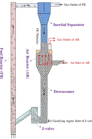
(4) Gas Outlet of FR. Inertial Separator OC Particles. Gas Outlet of AR. Air Reactor (AR). Fuel Reactor (FR). Air Inlet of AR. Downcomer. Gasifying Agent Inlet of J-valve. J-valve Gasifying Agent Inlet of FR. Figure 1. Schematic of the novel iG-CLC system. In our previous experimental studies, we had developed a novel iG-CLC system which mainly comprised a high-flux circulating fluidized bed (HFCFB) as the FR and a counter-flow moving bed (CFMB) as the AR, as shown in Figure 1.22 It should be noted that in our previous study,22 considering the cross directions with gas horizontally flowing into the AR and solids moving downwards in the AR, the AR was named as “cross-flow moving bed AR”. However, in view of. 4.

(5) the actual gas-solids contact with gas flowing upwards and solids moving downwards, it should be better to call the AR “counter-flow moving bed AR”. The HFCFB FR achieved intense turbulence, which could provide a favorable gas-solids contact and avoid the phenomenon of gas bypass via the bubbles, just like what typical CFB FRs17-19 can do. The unique feature of high-flux operation of the system could greatly increase the concentration and flow rate of solids in the FR, and enhance the gas-solids contact and reaction efficiencies. The AR was designed as a CFMB reactor because of its features of compact structure, low pressure drop, steady particle flow, and sufficient residence time of solids. In addition, as the location of the AR was arranged in the middle of the downcomer, the driving source of particle circulation in the whole iG-CLC system was only from the HFCFB, which was beneficial for the operation stability and adjustment flexibility. Although the experimental results show that the iG-CLC system could be operated under a favorable condition with stable solids circulation and effective solids separation, we also found that the power capacity of the system was limited by the carrying capacity of the gas flow in the AR, because the gas flow introduced to the AR determined the oxygen transported to the FR by the OCs, and further greatly influenced the reaction performance in the FR. In order to meet the high power capacity requirement of future industrial application, it was essential to improve the carrying capacity of the gas flow in the AR. Although extensive experimental studies on CLC had been carried out to investigate the running performance of the system, some important operational information, such as instantaneous flow behaviors and inner solids distributions, is still largely missing and rarely available. With the development of numerical techniques, computational fluid dynamics (CFD) has been accepted as a reliable approach to make up for the limitation of experimental methods, and further provides some forward guidance for deeper experimental studies.23-28 Previous publications on the CFD. 5.

(6) simulation studies of CLC mainly focused on gas-fueled CLC units29-39 and few were on the iGCLC systems. Mahalatkar et al.40 took the lead in developing a two dimensional model to investigate the flow and reaction performance in a BFB FR. Subsequently, Wang et al.41 established a CFB FR model together with an upgrade from two dimension to three dimension. However, in their work, the iG-CLC systems were simplified as a single FR, which could make the results inaccurate and insufficient, as the integration of different parts could influence the flow and reaction characteristics of the whole system. So far, few studies, if any, have been carried out on full loop iG-CLC simulations because of the complexities in model geometry and flow kinetics. Zhang et al.42 developed a quasi-three-dimensional full-loop iG-CLC model, including a spout fluidized bed FR, a cyclone separator, a downcomer, and a loop-seal, to investigate the multiphase flow and circulation dynamics in the system and the performance of a simplified reaction between CH4 and the OC. However, it was not feasible for continuous redox circulation of the OC in their work, as the AR was not included in their full loop model, which could lead to further limitations and/or inaccuracies in the whole system modeling. In the CLC simulations, the gas-solids flow behaviors are greatly influenced by modeling parameters such as the drag model and the specularity coefficient. Currently, researches focusing on the effects of drag models could be found in existing literatures. The Wen-Yu model,43 Gidaspow model44 and Syamlal-O’Brien model45 were carefully studied and commonly used in fluidized bed simulations.29-39 The simulation results agreed well with the experimental data with different drag models. As to the specularity coefficient, it reveals the roughness of the wall and depends on the material and geometry of the wall, the properties of the particle, and so on. By far, experimental studies on the specularity coefficient were almost unavailable in the open literature due to the difficulty in measurement, and the simulation studies on it were few, although it had. 6.

(7) great influence on the hydrodynamics. Wang et al.46 and Xue et al.47 chose the no-slip solid-wall boundary condition with the specularity coefficient value of unity, and Jin et al.48 and Sasic et al.49 applied the free-slip solid-wall boundary condition with the value of zero. However, Guan et al.37 and Wang et al.50 preferred to use the partial-slip solid-wall boundary conditions with different values between zero and unity. Overall, no generic modeling parameters of the drag model and the specularity coefficient are available in the existing studies, and thus, it is essential to study the effects of the modeling parameters in detail and finally choose a value which can well predict the gas-solids flow behaviors in the specific CLC system. In this study, a three dimensional full loop model was developed based upon our previous experimental apparatus.22 A series of CFD simulations were carried out to comprehensively investigate the hydrodynamic characteristics in the iG-CLC system. This model mainly comprised an HFCFB as the FR, a CFMB as the AR, an inertial separator, a J-valve and a downcomer. Moreover, a two-stage AR was first proposed in this work to improve the power capacity of the system. Compared to the previous studies, the main advances of this simulation work include: (1) successful establishment of a three dimensional full loop model for a novel iG-CLC system, (2) in-depth study of the effects of the modeling parameters on the solids flow behaviors, (3) predictions of detailed flow dynamics characteristics in the whole system, (4) successful increase of the power capacity in the optimized iG-CLC system.. 2. Mathematical model The Eulerian-Eulerian two-fluid model was applied to model the gas-solids flow behaviors in the iG-CLC system. The gas phase and solids phase were regarded as the primary phase and second phase, respectively, and the two phases were mathematically described as the fully. 7.

(8) interpenetrating continuum. The gas phase was modeled by the    turbulence model, and the solids phase was described by the kinetic theory of granular flow.. 2.1. Governing equations 2.1.1. Continuity equations   g  g     ( g  g vg )  0 t. (1).   s  s     ( s  s vs )  0 t. (2). where  denotes the volume fraction which is the space occupied by each phase (  g   s  1 )..   and v represent the density and the instantaneous velocity vector, respectively. The subscripts. g and s stand for the gas phase and the solids phase, respectively. 2.1.2. Momentum equations   g  g vg     ( g  g vg vg )   g pg     g   g  g g   (vs  vg ) t. (3).   s  s vs     ( s  s vs vs )   sps    s   s  s g   (vg  vs ) t. (4).  where g , p and  are the gravity acceleration, the pressure and the stress tensor, respectively..  is the momentum transfer coefficient between the gas and solids phases.. 2.2. Constitutive equations In order to close the governing equations, the momentum transfer coefficient between the gas and solids phases  , the stress-strain tensor of the gas phase  g and the solids phase  s were. 8.

(9) described by the constitutive equations which were derived from the physical properties of the gas and solids phases. 2.2.1. Inter-phase momentum transfer In the gas-solids flow, the drag force were determined by the product of the inter-phase momentum transfer coefficient  and the gas-solids slip velocity. Different drag models have been proposed to estimate the inter-phase momentum transfer coefficient  in the existing literature. The Wen-Yu model,43 Gidaspow model44 and Syamlal-O’Brien model45 got wide application therein. The Wen-Yu model43 was based on the settling experiments of particles in a liquid over a wide range of solids volume fractions, which was recommended for the dilute phase. The interphase momentum transfer coefficient  took the following form:.   0.75CD. 1   s  s  g  g  s ds. 1   s 2.65. (5). . (6). where. CD . . 24 0.687 1  0.15 g Re s   g Re s. Re s .    g g v s  v g d s. g. (7). where d s is the solids diameter, and  g is the gas phase shear viscosity. The Gidaspow model45 was a combination of the Wen-Yu43 model and the Ergun equation51, which can separately calculate the inter-phase momentum transfer coefficient  in the dilute phase and the dense phase. For the dilute phase with the gas volume fraction higher than 0.8, the. 9.

(10) Wen-Yu model was applied, while for the dense phase with gas volume fraction lower than 0.8, the Ergun equation was adopted:     s g  g vs  vg 2.65 0.75C D  g , ( g  0.8) ds       g s vs  v g  s2  g  , ( g  0.8) 150  d 2  1.75 d g s s . (8). The Syamlal-O’Brien model46 was based on the measurements of the terminal velocities of particles in the fluidized beds or settling beds:.   0.75C D.  s (1   s )  g 2. Vr d s.  g  s. (9). where CD is the drag function derived by Dalla Valle,52 and Vr is the ratio of the suspension falling velocity to the single particle terminal velocity:53  V  C D   0.63  4.8 r  Re   Vr . 1 a  0.06 Re  2 . 2. (10). 0.06 Re 2  0.12 Re2b  a   a 2  . (11). a  (1   s ) 4.14. (12). 1   s 2.65 ,   g  0.15 b 1.28 0.81   s  ,  g  0.15. (13). 2.2.2. Stress tensor of the gas phase The stress tensor of the gas phase  g can be expressed as:. . .   2   g   g  g vg  (vg )T   g  g   vg I 3. (14).  g   gl   gt. (15). 10.

(11) where,  g , gl. and gt are the gas phase shear viscosity, laminar viscosity and turbulent. viscosity, respectively. In this work, the standard    turbulence model was applied to compute the gas phase turbulent kinetic energy  and the dissipation rate of turbulent kinetic energy  . The turbulent viscosity gt can be calculated as a function of the  and  :.  gt   g C. 2 . (16). where C  is a constant which is set as 0.09. The turbulence kinetic energy  and its rate of dissipation  are obtained from the following transport equations:.   g  g     ( g  g vg )    ( g  gt  )   g G   g  g   g  g  t . (17).   g  g     ( g  g vg )    ( g  gt  )   g  (C1G  C2  g )   g  g  t  . (18). In Eqs. (17) and (18),  k and   are the turbulence exchange terms between the gas and solids phases. Gk is the production of turbulent kinetic energy. The constants C1 =1.44 and C 2 =1.92. The turbulent Prandtl numbers  k = 1.0 and   = 1.3. 2.2.3. Stress tensor of the solids phase The solids phase was described by the kinetic theory of granular flow which was derived from the kinetic theory of gases. Equivalent to the thermodynamic temperature for gases, the granular temperature  was introduced as a measure for the energy of the particle fluctuating velocity.45 The stress tensor of the solids phase  s is given by:54. 11.

(12)    2  s   s  s (vs  vsT )   s ( s   s )  vs I 3. (19). where  s and  s are the solids bulk viscosity and the solids shear viscosity, respectively, which can be written in the following forms:55. 4   s   s  s d s g 0 (1  e) 3 . (20). 4  10s d s   4 p sin   s   s s d s g0 (1  e)  1   s g0 (1  e)  s  5  96 s g0 (1  e)  5 2 I2D  2. (21). where g 0 is the radial distribution function:.    1 / 3  g 0  1   s      s , max    . 1. (22). The conservation equation of the granular temperature derived from the kinetic theory of granular flow takes the following form:   s  s     ( s  s vs)  2   ps I   s  : vs        s  s   t 3  . (23). where  is the granular temperature, p s the solids pressure,  the diffusion coefficient for granular energy,  s the dissipation of fluctuating energy due to the inelastic collisions, and  s the exchange of fluctuating energy between the gas and solids phases: . 1    vs  v s  3. (24). ps   s  s   2 g 0 s2  s (1  e). 150  s d s    384(1  e) g0. (25) 2.   6  2 1  5 (1  e) g0 s   2  s s d s g0 (1  e)   . (26). 12.

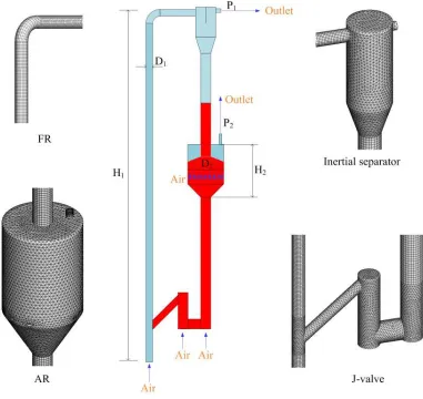
(13)  s  3(1  e 2 ) s  s g 0 s ( 2. 4 ds. s    vs ) .  s  3  . (27) (28). 2.3. Geometry and mesh As shown in Figure 2, an iG-CLC full loop model based on our previous cold experimental apparatus22 was developed in this study, which was mainly composed of an HFCFB FR (D1=60 mm, H1=5.8 m), a CFMB AR (D2=418 mm, H2=0.7 m) , a J-valve, an inertial separator and a downcomer.. Figure 2. Sketch and grids of the iG-CLC full loop model.. 13.

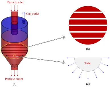
(14) Figure 3 specifically shows the schematic drawing and model processing of the CFMB AR. As shown in Figure 3a, the AR mainly comprised a cylindrical channel, a cone channel, a particle inlet, a particle outlet, a gas distributor, and a gas outlet. From Figure 3b, we can further observe the gas distributor were composed of five parallel tubes which were placed in the horizontal crosssection of the cylindrical channel. In the experimental system, each tube of the gas distributor was cylindrical with 20-40 nozzles arranged symmetrically at the bottom with an angle of 90o. However, in order to reduce the model complexity and computational cost, each tube of the gas distributor in the model was simplified to a semi-cylindrical tube, and the air was injected into the AR from the flank uniformly and vertically during the simulation process (see Figure 3c).. Figure 3. Schematic drawing and model processing of the CFMB AR: (a) inside view, (b) top view of the gas distributor, (c) side view of one tube of the gas distributor.. 14.

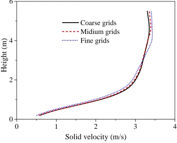
(15) As for meshing, the computational domain was divided into several parts so as to obtain most structured grid cells. Most parts of the cylindrical volumes (e.g., the FR and the downcomer) were meshed with hexahedrons, while the connecting parts, the J-valve, the inertial separator and the AR were meshed with tetrahedrons. The grid independence tests were carried out with three computational domains of 0.141, 0.282, and 0.414 million cells. Figure 4 shows the distributions of solids velocity in the FR predicted with the three different computational grids. It indicates that the simulation results reached a good agreement, and the maximum relative error was less than 10%, implying the gird independence was verified. Therefore, in view of the time cost, the medium grid resolution of 281 849 cells was finally chosen in this work.. Height (m). 6 Coarse grids Midium grids Fine grids. 4. 2. 0 0. 1. 2. 3. 4. Solid velocity (m/s) Figure 4. Axial distributions of solids velocity in the FR with different computational grids.. 15.

(16) 2.4. Data evaluation 2.4.1. FR fluidizing number Nf represents the FR fluidizing number which is defined as the ratio between the superficial gas velocity of the FR and the minimum fluidizing velocity of the OC.22. Nf . Uf U min. (29). where Uf , Umin are the superficial gas velocity of the FR and the minimum fluidizing velocity of the OC, respectively. 2.4.2. AR fluidizing number Na represents the AR fluidizing number which is defined as the ratio between the superficial gas velocity of the AR and the minimum fluidizing velocity of the OC.22 Na . Ua U min. (30). where Ua is the superficial gas velocity of the AR.. 2.5. Numerical procedure In this study, the phase coupled Semi-Implicit Method for Pressure-Linked Equations (PCSIMPLE) algorithm, which is an extension of the SIMPLE algorithm to the multiphase flow field, was applied to deal with the pressure-velocity coupling and correction. All the differential equations were solved by a finite volume method. The second order upwind scheme was chosen for the momentum equations while the first order upwind scheme was chosen for all the other governing equations. The convergence criterion was set as 1×10-4. A time step of 5×10-4 s and 5 iterations per time step were chosen as the parameters for iteration.. 16.

(17) The velocity-inlet boundary condition was applied for all of the inlets. The pressure-outlet boundary condition was selected for the two outlets of the system. At the walls, the no-slip wall condition was adopted for the gas phase. The Johnson and Jackson slip boundary condition56 was chosen for the solid phase, in which the tangential velocity  s, w and solids granular temperature  w at the wall take the following forms:.  s ,w  . 6 s s ,max.  s ,w. 3 s s g 0  n. 3 s sus , slip g03 / 2 k w w     w n 6 s , max w. w . . . 3 1  ew  s  s g03 / 2 4 s , max 2. (31). (32). (33). where  is the specularity coefficient, and ew is the restitution coefficient of the solid-wall collisions. The value of ew was set as 0.9 in this study.37, 39 Initially, about 150 kg of the OC particles were packed in the J-valve, lower downcomer, AR and part of the upper downcomer with an initial solids volume fraction of 0.6 while the maximum packing of solids was set as 0.63. The OC in this study was an iron ore from China, which has an apparent density of 2558 kg/m3 with a mean diameter of 0.65 mm. The gas used was air with a density of 1.293 kg/m3 and a viscosity of 1.78×10-5 pa·s.. 3. Results and discussion This work mainly devoted to the development of a three dimensional full loop iG-CLC model, the study on the effects of modeling parameters, and the research on the gas-solids flow characteristics and operating mechanism of the novel iG-CLC system proposed by us. Moreover, a two-stage AR was first proposed to optimize the iG-CLC system so as to increase the power. 17.

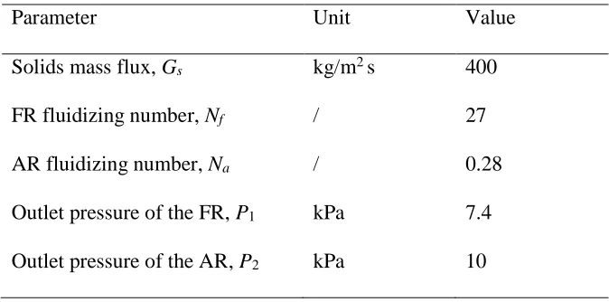
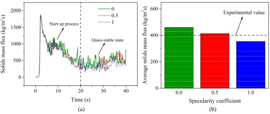
(18) capacity. The simulations were carried out under the same operating conditions as those applied in our previous experiments.22 Table 1 lists the detailed operating parameters. Table 1. Operating parameters applied to the simulation. Parameter. Unit. Value. Solids mass flux, Gs. kg/m2 s. 400. FR fluidizing number, Nf. /. 27. AR fluidizing number, Na. /. 0.28. Outlet pressure of the FR, P1. kPa. 7.4. Outlet pressure of the AR, P2. kPa. 10. 3.1. Effect of the specularity coefficient The specularity coefficient is defined to be the fraction of the relative tangential momentum transfer through solid-wall collisions, which specifies the roughness of the wall.48 The value of zero represents zero shear at the wall, which means the completely smooth wall condition or the free-slip solid-wall boundary condition. The value of unity means perfectly diffuse collision between the particles and the wall or the no-slip solid-wall boundary condition. The values can vary between zero and unity, where the roughness of the wall increases with an increase in the value. In this study, three values of 0, 0.5 and 1 were set to account for different slip boundary conditions so as to obtain an appropriate specularity coefficient for the 3D full loop model. Figure 5 shows the profiles of the solids mass fluxes with different specularity coefficients, where the solids mass fluxes were sampled from a horizontal cross-section set in the FR. In Figure 5a, we observed intense fluctuations of solids mass fluxes between 0 s and 20 s of the computational time, which could be regarded as the start-up process. Afterwards, the solids mass. 18.

(19) fluxes fluctuated around a constant value, indicating the achievement of quasi-stable solids circulation in the whole system. Meanwhile, the unique high flux (>200 kg/m2s) operation was innovatively realized in the CFB FR, which could enhance the gas-solids contact and reaction performance.. (a). (b). Figure 5. Profiles of the solids mass fluxes with different specularity coefficients: (a) solids mass flux fluctuations with the computational time, (b) time-averaged solids mass fluxes at the quasistable state. For more accurate analysis of the effects of the specularity coefficients, the time-averaged solids mass fluxes were obtained from the quasi-stable state between 20 s and 40 s with the interval of 0.1 s, as shown in Figure 5b. It can be seen that compared with the experimental value, the specularity coefficient of 0 overpredicted the average solids mass flux, and the specularity coefficient of 1 underpredicted it. The value of 0.5 shows a reasonable result with the relative error less than 5%, and hence, the specularity coefficient of 0.5 was finally adopted for the 3D full-loop model, which was the same as the value Wang et al.50,57 applied in their simulations for CLC systems.. 19.

(20) Z/H=0.2. Z/H=0.2. Z/H=0.5. Z/H=0.5. Figure 6. Radial profiles of the time-averaged solids volume fraction and velocity in the riser with different specularity coefficients. In order to further investigate the influence mechanism of the specularity coefficient, the radial profiles of the time-averaged solids volume fraction and velocity under the quasi-stable state in the riser were studied, as shown in Figure 6. Different specularity coefficients predicted similar solids distribution trends at the same height, which presents larger solids volume fraction and smaller velocity in the near-wall region, compared with those in the center region. In the bottom section of the riser (Z/H=0.2), the radial solids volume fraction and velocity distributions show obvious asymmetry due to the influence of the solids inlet set in the right side of the riser. In the middle section of the riser (Z/H=0.5), the gas-solids flow had been fully developed, and hence, the. 20.

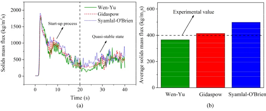
(21) radial solids concentration distribution was more homogeneous just with slight difference between the near-wall region and the center region, and the central high solids velocity area was obviously enlarged. In Figure 6, for clearer presentation, the solids velocity distribution in the near-wall region was zoomed to a certain extent. With an increase in the specularity coefficient, the solids volume fraction increased, while the solids velocity decreased. This was due to the larger resistance at the wall leading to the inhibition of the solids upward movement. Hence, the solids mass flux decreased with an increase in the specularity coefficient, as shown in Figure 5b.. 3.2. Effect of the drag model. (a). (b). Figure 7. Profiles of the solids mass fluxes with different drag models: (a) solids mass flux fluctuations with the computational time, (b) time-averaged solids mass fluxes at the quasi-stable state. Figure 7 shows the profiles of solids mass fluxes with different drag models, when the specularity coefficient was set as 0.5. Figure 7a illustrates the solids mass flux fluctuations with the computational time, which presents the similar trends as those shown in the Figure 5a. Figure. 21.

(22) 7b presents the time-averaged solids mass fluxes at the quasi-stable state. The Syamlal-O’Brien drag model predicted the largest solids mass flux, and the Wen-Yu model presented the minimum value. The Gidaspow model reported the closest value to the experimental result with the relative error less than 5%. In the existing literature, Jung et al.29,31,35 also chose the Gidaspow drag model in the CLC simulation. Hence, the Gidaspow drag model was finally chosen in this full loop model for further study.. Z/H=0.2. Z/H=0.2. Z/H=0.5. Z/H=0.5. Figure 8. Radial profiles of time-averaged solids volume fraction and velocity in the riser with different drag models.. 22.

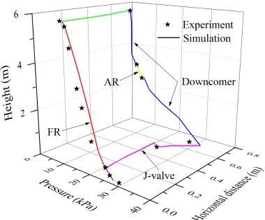
(23) In order to study the effects of the drag model on the solids movement in the riser, the radial profiles of solids concentration and velocity at different heights were studied in detail. As shown in Figure 8, the three drag models predicted similar solids volume fraction and velocity distribution trends. However, the Syamlal-O’Brien model predicted the largest volume fraction and velocity, which led to the largest solids mass flux, as shown in Figure 7b. The Wen-Yu model reported the smallest volume fraction and velocity, which caused the smallest solids mass flux accordingly.. 3.3. Model validation and flow patterns of the whole system. The feasibility of the three dimensional full loop model was further verified by comparing the pressure profile of the iG-CLC cold system between experimental data22 and simulation predictions, as shown in Figure 9. Here, the point at the left bottom of the FR was defined as the origin coordinate of the height and horizontal distance in this figure. In the FR, the pressure decreased almost linearly with the increasing bed height. Similarly, the pressure in the downcomer showed proportional decrease trend along the bed height. However, the average gradient of the pressure variation in the FR was smaller than that in the downcomer due to the lower solids holdups. As for the AR, the pressure only had a slight drop of about 2 kPa between the inlet and outlet, which was beneficial for the stability of gas-solids flow. The maximum pressure occurred in the intersection part of the J-valve and the lower downcomer, indicating that the J-valve was the driving source of solids circulation in the whole system. In general, the simulation results agreed well with the experimental data, and the maximum relative error was less than 15%. Hence, the three dimensional full loop model developed in this study should be reasonable for the further predictions of the flow characteristics in our iG-CLC system.. 23.

(24) Figure 9. Comparisons of the pressure profiles of the iG-CLC cold system between experimental data and simulation predictions. Figure 10 shows the instantaneous solids holdup distributions of the whole system at the quasi-stable state. It could be observed that the OC particles were driven and lifted by the gas stream in the FR, and then were separated by the inertial separator into the downcomer and the AR. Further, they were sent back to the FR via the J-valve. The bed height above the AR almost kept constant from 40 s to 60 s, indicating the quasi-stable solids circulation along the path of “Jvalve - FR - Inertial separator - Downcomer - AR - Downcomer - J-valve”. Meanwhile, the particles packed above the AR was able to act as the material seal to restrain the gas leakage between the inertial separator and the AR. The FR and the AR achieved intense turbulence flow and steady near plug flow, respectively. In the J-valve, the bubbling fluidization structure was. 24.

(25) realized in the vertical pipe to ensure the continuous transport of the particles from the downcomer to the FR with the help of the overflow.. 0.60 0.55 0.50 0.45 0.40 0.35 0.30 0.25 0.20 0.15 0.10 0.05. Figure 10. Instantaneous solids holdup distributions in the iG-CLC system.. 3.4. Flow characteristics of the FR For CFB typed FRs, the solids holdup is a key operating parameter affecting the gas-solids contact and reaction efficiencies. The radial solids distributions had been shown in section 3.1 and section 3.2. Figure 11 shows the axial profiles of the predicted solids holdups in the FR. It can be. 25.

(26) seen that the solids holdup generally decreased along the FR height, but with a slight increase near the exit. Meanwhile, the solids holdup at any height was over 0.05, demonstrating the positive effects of high solids flux on the gas-solids contact, and further the gas-solids reaction efficiency. Hence, under a high-flux operating condition, the gas-solids reaction performance could be greatly enhanced in terms of CO2 yield, carbon capture efficiency, fuel conversion, and so on. It should be noted that the application of the two-fluid model to different apparatus parts, including the HFCFB FR, CFMB AR, downcomer, inertial separator and J-valve, so as to achieve full loop iGCLC simulations inevitably led to a certain calculation deviation of flow characteristics, such as the lower height of the bottom dense region compared to that in the experiment.22. Height (m). 6. 4. 2. 0 0.00. 0.05. 0.10. 0.15. 0.20. 0.25. 0.30. Solids volume fraction (-) Figure 11. Axial profiles of the predicted solids holdups in the FR.. 3.5. Flow characteristics of the AR. 26.

(27) For a moving bed as the AR, the achievement of a uniform distribution and smooth flow of solids is crucial, which can directly influence the effect of oxygen transfer from the air to the reduced oxygen carrier for regeneration.. Figure 12. Radial profiles of the predicted solids volume fraction and velocities in the AR at different bed heights. Figure 12 shows the radial profiles of the predicted solids volume fractions in the AR at different bed heights. It should be noted that the cross section where the gas distributor located was defined as the reference plane of the AR, that is, the bed height HAR for this plane was set to be zero. It can be observed that, at a given bed height, the solids volume fraction in the center region was slightly lower than that in the near-wall region. This is believed to be related to the solids flow behaviors from the large-diameter AR to the small-diameter downcomer and the wall resistance to the solids. In addition, the solids volume fraction rose slightly along the bed height of AR, indicating the effect of loosening due to the solids downward flow was more obvious at the bottom region of the AR. Generally, the solids distribution in the CFMB AR was quasi-uniform, which should be beneficial to the contact and reaction efficiencies between the air and the OC. It can also be found that the spatial distributions of the solids velocities presented reverse trends to. 27.

(28) those of the solids volume fractions in both of the radial and axial directions. On the other hand, the average residence time of solids derived from the mean solids velocity in the AR was sufficient time to ensure the contact and reaction efficiencies between the air and OC.. Q < Qc. Q ≈ Qc. Q > Qc. Figure 13. Different flow states in the CFMB AR with an increase in the inlet gas flow Q. The gas-solids flow behaviors in the CFMB AR were greatly influenced by the inlet gas flow Q. In order to ensure the stable flow state in the AR, the gas flow introduced to the AR should be lower than a limit value which could be defined as the carrying capacity of the gas flow Qc. Figure 13 shows different flow states in the CFMB with an increase in the inlet gas flow Q. It can be seen that under the safe gas flow condition (Q < Qc), the AR was operated under the near plug flow state, where uniform solids distribution could ensure favorable gas-solids contact, high reaction efficiency and stable solids circulation. With the increase of the AR inlet gas flow (Q ≈ Qc), small bubbles were observed around the gas inlets, which wouldn’t influence the regeneration of the reduced OCs due to the sufficient solids resistance time in the AR. However, when the inlet gas flow exceeded the critical value (Q > Qc), the AR was operated under the bubbling fluidization. 28.

(29) regime. Lots of bubbles in the reactor not only provided shortcuts for gas to flow through, causing a decrease in gas-solids contact and reaction efficiency, but also led to the bed expansion which increased the risk of solids exiting from the AR outlet. The above observations were consistent with our previous experimental studies.22 Overall, the different flow states in the CFMB AR indicate that lots of bubbles in the reactor should be avoided in case of adversely affecting sufficient gas-solids contact and stable solids circulation.. 3.6. Operating performance of the optimized iG-CLC system In order to improve the power capacity of the iG-CLC system, it was essectial to fundamentally increase the oxygen transported from the AR to the FR. That’s to say, the carrying. 3. Carrying capacity of the AR gas flow (Nm /h). capacity of the gas flow Qc in the AR should be enhanced. 280 240 200 Upper CFMB. 160 120 80. Lower CFMB. 40 0. Primary system. Optimized system. Figure 14. Comparison of the carrying capacity of the AR gas flow Qc between the primary system and the optimized system. We proposed a two-stage AR with two identical CFMBs connected in series which also located in the middle of the downcomer. Figure 14 shows the comparison of the carrying capacity. 29.

(30) of the AR gas flow Qc between the primary system and the optimized system. It can be seen that Qc of the optimized system was about two times as much as that of the primary one, which verified the improvement effect of the two-stage AR on the carrying capacity of the gas flow Qc. This means the power capacity of the iG-CLC system could be successfully doubled.. 50 s. 60 s. 70 s. Figure 15. Instantaneous solids distribution in the optimized iG-CLC system. Figure 15 shows the instantaneous solids distribution in the optimized iG-CLC system coupled with a two-stage AR. The gas introduced to each AR was the same as that applied in the model for the primary iG-CLC system. It can be seen that two CFMBs were both operated in near. 30.

(31) plug flow regimes, where the homogeneous solids distribution could ensure the steady gas-solids contact and stable regeneration reaction of the reduced OCs with the air. Meanwhile, the two-stage configuration enabled staged OC regeneration and extended the solids residence time, which could facilitate the oxidization of the reduced OCs.. FR. 17. Pressure drop (kPa). 16 15 Upper CFMB of AR. 2 1 0. Lower CFMB of AR. 2 1 0 50. 60. 70. 80. 90. 100. Time (s) Figure 16. Pressure drop fluctuations with the computational time in the FR and the two-stage AR. In order to further investigate the solids circulation stability in the optimized iG-CLC system coupled with a two-stage AR, the pressure drop fluctuations in the CFB and two CFMBs were monitored, as shown in Figure 16. It can be seen that the FR pressure drop fluctuated around 16.0 kPa, indicating the quasi-stable state was achieved in the system. As to the AR, the pressure drops of the upper CFMB and the lower CFMB almost stayed constant at the value of about 1.0 kPa and 1.2 kPa, respectively. This indicates the steady gas-solids flow with low pressure drop was. 31.

(32) successfully realized in the two-stage AR, which was beneficial for improving the running stability of the whole system. Due to the intense turbulence in the HFCFB FR and the steady near plug flow in the two-stage AR, the amplitudes of the pressure drop in the FR were much larger than those in the AR. Overall, the differential pressure fluctuations reflected that the optimized iG-CLC system was able to realize stable solids circulation and favorable gas-solids contact. As the feasibility of the proposed two-stage AR was just preliminarily verified based on the model of the previous iG-CLC system, further studies should be carried out to validate the 3D full loop model for the optimized iG-CLC system. On one hand, the two-stage AR will be coupled into the experimental apparatus, and the experimental measurement accuracy should be improved. On the other hand, the modeling parameters (e.g. gas-solids collision restitution coefficient, drag model, and specularity coefficient) should be checked to minimize the relative error between the experimental results and the simulation predictions.. 4. Conclusions A comprehensive three dimensional full loop numerical model has been developed to simulate the flow dynamics characteristics of a novel in situ gasification chemical looping combustion (iGCLC) system. This model is mainly composed of a high-flux circulating fluidized bed (HFCFB) riser as the fuel reactor (FR), a counter-flow moving bed (CFMB) as the air reactor (AR), an inertial separator, a J-valve and a downcomer. A two-stage AR was first proposed to enhance the power capacity of the system. The effects of the modeling parameters on the solids mass flux and solids distribution were studied in detail. The modeling results have presented favorable operation performance in terms of gas-solids flow behaviors and pressure distribution. The following conclusions can be drawn from the present study: (1) The Gidaspow drag model and the specularity coefficient of 0.5 were suitable for the three. 32.

(33) dimensional full loop iG-CLC model to predict reasonable gas-solids flow behaviors. (2) The continuous and stable solids circulation was successfully realized along the path of “Jvalve - FR - Inertial separator - Downcomer - AR - Downcomer - J-valve”. The high-flux solids circulation was innovatively achieved in the aspect of the full loop iG-CLC simulations to enhance the performances of reaction and heat transfer of the oxygen carrier. The FR and AR achieved intense turbulence and steady near plug flow, respectively. (3) The power capacity of the iG-CLC system was successfully increased by coupling a two-stage AR. In addition, the optimized system also exhibited continuous solids circulation, reasonable pressure distribution and favorable operation performance. AUTHOR INFORMATION Corresponding Author * Email: [email protected] (Baosheng Jin) * Email: [email protected] (Yong Zhang) Notes The authors declare no competing financial interest ACKNOWLEDGMENT This work has been financially supported by the National Natural Science Foundation of China (51676038, 51741603, and 51276038), Natural Science Foundation of Jiangsu Province (BK20170669), Fundamental Research Funds for the Central Universities, and Guangdong Provincial Key Laboratory of New and Renewable Energy Research and Development (Y707s41001).. 33.

(34) REFERENCES (1) Fan, LS. Chemical Looping Systems for Fossil Energy Conversions; Wiley-AIChE: New York, 2010. (2) Lyngfelt, A.; Leckner, B.; Mattisson, T. A fluidized-bed combustion process with inherent CO2 separation; application of chemical-looping combustion. Chem. Eng. Sci. 2001, 56, 31013113. (3) Abad, A.; Mattisson, T.; Lyngfelt, A.; Rydén, M. Chemical-looping combustion in a 300W continuously operating reactor system using a manganese-based oxygen carrier. Fuel 2006, 85, 1174-1185. (4) Mattisson, T.; García-Labiano, F.; Kronberger, B.; Lyngfelt, A.; Adánez, J.; Hofbauer, H. Chemical-Looping Combustion using syngas as fuel. Int. J. Greenhouse Gas Control 2007, 1, 158-169. (5) Abad, A.; Mattisson, T.; Lyngfelt, A.; Johansson, M. The use of iron oxide as oxygen carrier in a chemical-looping reactor. Fuel 2007, 86, 1021-1035. (6) Cao, Y.; Pan, WP. Investigation of Chemical looping combustion by solid fuels, 1 Process analysis. Energy Fuels 2006, 20, 1836-1844. (7) Berguerand, N.; Lyngfelt, A. Design and operation of a 10 kWth chemical-looping combustor for solid fuels-testing with South African coal. Fuel 2008, 87, 2713-2726. (8) Leion, H.; Mattisson, T.; Lyngfelt, A. Solid Fuels in Chemical-Looping Combustion. Int. J. Greenhouse Gas Control 2008, 2, 180-193. (9) Shen, LH.; Wu, JH.; Xiao, J. Experiments on chemical looping combustion of coal with a NiO based oxygen carrier. Combust. Flame 2009, 156, 721-728. (10) Xiao, R.; Song, QL.; Song, M.; Lu, Z. J.; Zhang, S.; Shen, LH. Pressurized chemical-looping. 34.

(35) combustion of coal with an iron ore-based oxygen carrier. Combust. Flame 2010, 157, 114011. (11) Abad, A.; Gayán, P.; de Diego, LF.; García-Labiano, F.; Adánez, J. Fuel reactor modelling in chemical-looping combustion of coal, 1. Model formulation. Chem. Eng. Sci. 2013, 87, 277293. (12) García-Labiano, F.; de Diego, LF.; Gayán, P.; Abad, A.; Adánez, J. Fuel reactor modelling in chemical-looping combustion of coal, 2-simulation and optimization. Chem. Eng. Sci. 2013, 87, 173-182. (13) Cuadrat, A.; Abad, A.; Gayán, P.; de Diego, LF.; García-Labiano, F.; Adánez, J. Theoretical approach on the CLC performance with solid fuels, optimizing the solids inventory. Fuel 2012, 97, 536-551. (14) Lyngfelt, A. Chemical-looping combustion of solid fuels-status of development. Appl. Energy 2014, 113, 1869-1873. (15) Thon, A.; Kramp, M.; Hartge, EU.; Heinrich, S.; Werther, J. Operational experience with a system of coupled fluidized beds for chemical looping combustion of solid fuels using ilmenite as oxygen carrier. Appl. Energy 2014, 118, 309-317. (16) Bayham, S.; McGiveron, O.; Tong, A.; Chung, E.; Kathe, M.; Wang, D.; Zeng, L.; Fan, LS. Parametric and dynamic studies of an iron-based 25-kWth coal direct chemical looping unit using sub-bituminous coal. Appl. Energy 2015, 145, 354-363. (17) Adánez, J.; Abad, A.; Perez-Vega, R.; de Diego, LF.; García-Labiano, F.; Gayán, P. Design and Operation of a Coal-fired 50 kWth Chemical Looping Combustor. Energy Procedia 2014, 63, 63-72. (18) Markström, P.; Linderholm, C.; Lyngfelt, A. Operation of a 100 kW chemical-looping. 35.

(36) combustor with Mexican petroleum coke and Cerrejón coal. Appl. Energy 2014, 113, 18301835. (19) Ma, J.; Zhao, H.; Tian, X.; Wei, Y.; Rajendran, S.; Zhang, Y.; Bhattacharya, S.; Zheng, C. Chemical looping combustion of coal in a 5 kWth interconnected fluidized bed reactor using hematite as oxygen carrier. Appl. Energy 2015, 157, 304-313. (20) Ströhle, J.; Orth, M.; Epple, B. Design and operation of a 1 MWth chemical looping plant. Appl. Energy 2014, 113, 1490-1495. (21) Xiao, R.; Chen, L.; Saha, C.; Zhang, S.; Bhattacharya, S. Pressurized chemical-looping combustion of coal using an iron ore as oxygen carrier in a pilot-scale unit. Int. J. Greenhouse Gas Control 2012, 10, 363-373. (22) Wang, X.; Jin, B.; Liu, H.; Wang, W.; Liu, X.; Zhang, Y. Optimization of in-situ Gasification Chemical Looping Combustion through Experimental Investigations with a Cold Experimental System. Ind. Eng. Chem. Res. 2015, 54, 5749-5758. (23) Yu, L.; Lu, J.; Zhang, XP.; Zhang, SJ. Numerical simulation of the bubbling fluidized bed coal gasification by the kinetic theory of granular flow (KTGF). Fuel 2007, 86, 722-734. (24) Zhong, W.; Jin, B.; Zhang, Y.; Wang, X.; Xiao, R. Fluidization of biomass particles in a gassolid fluidized bed. Energy Fuels 2008, 22, 4170-4176. (25) Wang, XF.; Jin, BS.; Zhong, WQ. Three-dimensional simulation of fluidized bed coal gasification. Chem. Eng. Process. 2009, 48, 695-705. (26) Chen, XZ.; Shi, DP.; Gao, X.; Luo, ZH. A fundamental CFD study of the gas-solid flow field in fluidized bed polymerization reactors. Powder Technol. 2011, 205, 276-288. (27) Zhou, W.; Zhao, CS.; Duan, LB.; Qu, CR.; Chen, XP. Two-dimensional computational fluid dynamics simulation of coal combustion in a circulating fluidized bed combustor. Chem. Eng.. 36.

(37) J. 2011, 166, 306-314. (28) Wang, X.; Jin, B.; Wang, Y.; Hu, C. Three-dimensional multi-phase simulation of the mixing and segregation of binary particle mixtures in a two-jet spout fluidized bed. Particuology 2015, 22, 185-193. (29) Jung, J.; Gamwo, IK. Multiphase CFD-based models for chemical looping combustion process, fuel reactor modeling. Powder Technol. 2008; 183, 401-409. (30) Deng, ZG.; Xiao, R.; Jin, BS.; Song, QL.; Huang, H. Multiphase CFD modeling for a chemical looping combustion process (fuel reactor). Chem. Eng. Technol. 2008, 31, 17541766. (31) Kruggel-Emden, H.; Rickelt, S.; Stepanek, F.; Munjiza, A. Development and testing of an interconnected multiphase CFD-model for chemical looping combustion. Chem. Eng. Sci. 2010, 65, 4732-4745. (32) Mahalatkar, K.; Kuhlman, J.; Huckaby, ED.; O'Brien, T. Computational fluid dynamic simulations of chemical looping fuel reactors utilizing gaseous fuels. Chem. Eng. Sci. 2011, 66, 469-479. (33) Wang, S.; Liu, G.; Lu, H.; Chen, J.; He, Y.; Wang, J. Fluid dynamic simulation in a chemical looping combustion with two interconnected fluidized beds. Fuel Process. Technol. 2011, 92, 385-393. (34) Wang, S.; Yang, Y.; Lu, H.; Wang, J.; Xu, P.; Liu, G. Hydrodynamic simulation of fuelreactor in chemical looping combustion process. Chem. Eng. Res. Des. 2011, 89, 1501-1510. (35) Harichandan, AB.; Shamim, T. CFD analysis of bubble hydrodynamics in a fuel reactor for a hydrogen-fueled chemical looping combustion system. Energ. Convers. Manage. 2014, 86, 1010-1022.. 37.

(38) (36) Parker, JM. CFD model for the simulation of chemical looping combustion. Powder Technol. 2014, 265, 47-53. (37) Guan, Y.; Chang, J.; Zhang, K.; Wang, B.; Sun, Q. Three-dimensional CFD simulation of hydrodynamics in an interconnected fluidized bed for chemical looping combustion. Powder Technol. 2014, 268, 316-328. (38) Peng, Z.; Doroodchi, E.; Alghamdi, YA.; Shah, K.; Luo, C.; Moghtaderi, B. CFD-DEM simulation of solid circulation rate in the cold flow model of chemical looping systems. Chem. Eng. Res. Des. 2015, 95, 262-280. (39) Geng, C.; Zhong, W.; Shao, Y.; Chen, D.; Jin, B. Computational study of solid circulation in chemical-looping combustion reactor model. Powder Technol. 2015, 276, 144-155. (40) Mahalatkar, K.; Kuhlman, J.; Huckaby, ED.; O'Brien, T. CFD simulation of a chemicallooping fuel reactor utilizing solid fuel. Chem. Eng. Sci. 2011, 66, 3617-3627. (41) Wang, X.; Jin, B.; Zhang, Y.; Zhang, Y.; Liu, X. Three Dimensional Modeling of a CoalFired Chemical Looping Combustion Process in the Circulating Fluidized Bed Fuel Reactor. Energy Fuels 2013, 27, 2173-2184. (42) Zhang, Z.; Zhou, L.; Agarwal, R. Transient simulations of spouted fluidized bed for coaldirect chemical looping combustion. Energy Fuels 2014, 28, 1548-1560. (43) Wen, CY.; Yu, Y. Mechanics of fluidization. Chem. Eng. Prog. Symp. Ser. 1966, 6, 100-101. (44) Gidaspow, D. Multiphase flow and fluidization: continuum and kinetic theory descriptions; Academic Press Inc.: Boston,1994. (45) Syamlal, M.; O'Brien, T. Simulation of granular layer inversion in liquid fluidized beds. Int. J. Multiphase Flow 1988, 14, 473-481. (46) Wang, X. Y.; Jiang, F.; Xu, X.; Fan, B. G.; Lei, J.; Xiao, Y. H. Experiment and CFD. 38.

(39) simulation of gas-solid flow in the riser of dense fluidized bed at high gas velocity. Powder Technol. 2010, 199, 203-212. (47) Xue, Q.; Heindel, T. J.; Fox, R. O. A CFD model for biomass fast pyrolysis in fluidized-bed reactors. Chem. Eng. Sci. 2011, 66, 2440-2452. (48) Jin, B.; Wang, X.; Zhong, W.; Tao, H.; Ren, B.; Xiao, R. Modeling on high-flux circulating fluidized bed with Geldart group B particles by kinetic theory of granular flow. Energy Fuels 2010, 24, 3159-3172. (49) Sasic, S.; Johnsson, F.; Leckner, B. Inlet boundary conditions for the simulation of fluid dynamics in gas-solid fluidized beds. Chem. Eng. Sci. 2006, 61, 5183-5195. (50) Wang, S.; Liu, G.; Lu, H.; Xu, P.; Yang, Y.; Gidaspow, D. A cluster structure-dependent drag coefficient model applied to risers. Powder technol. 2012, 225, 176-189. (51) Ergun, S. Fluid flow through packed columns. Chem. Eng. Prog. 1952, 48, 89-94. (52) DallaValle, J. Micrometrics: The technology of fine particles; Pitman, 1948. (53) Garside, J.; Al-Dibouni, M. R. Velocity-voidage relationships for fluidization and sedimentation in solid-liquid systems. Ind. Eng. Chem. Process Des. Dev. 1977, 16, 206-214. (54) Ding, J.; Gidaspow, D. A bubbling fluidization model using kinetic theory of granular flow. AIChE J. 1990, 36, 523-538. (55) Lun, CKK.; Savage, SB.; Jerey, DJ.; Chepurniy, N. Kinetic Theories for Granular FlowInelastic Particles in Couette-flow and Slightly Inelastic Particles in a General Flow field. J. Fluid Mech. 1984, 140, 223-256. (56) Johnson, P. C.; Jackson, R. Frictional-collisional constitutive relations for particulate flows and their application to clusters. J. Fluid Mech. 1987, 176, 67-93. (57) Wang, S.; Lu, H.; Zhao, F.; Liu, G. CFD studies of dual circulating fluidized bed reactors for. 39.

(40) chemical looping combustion processes. Chem. Eng. J. 2014, 236, 121-130. Gas Outlet of FR. iG-CLC Schematic. Numerical Model. Inertial Separator Gas Outlet of AR. Air Reactor (AR). Fuel Reactor (FR). Air Inlet of AR. Downcomer. Gasifying Agent Inlet of J-valve. J-valve Gasifying Agent Inlet of FR. For Table of Contents Only. 40.

(41)

No results found