Combining Spatial and Parametric Working Memory in a
Dynamic Neural Field Model
Weronika Wojtak, Stephen Coombes, Estela Bicho, Wolfram Erlhagen
IN:
Artificial Neural Networks and Machine Learning – ICANN 2016
Volume 9886 of the series
Lecture Notes in Computer Science
, pp 411-418
Date: 13 August 2016
memory in a dynamic neural field model
Weronika Wojtak1,3,⋆, Stephen Coombes2,
Estela Bicho1, and Wolfram Erlhagen3
1
Research Centre Algoritmi, University of Minho, Portugal
{w.wojtak,estela.bicho}@dei.uminho.pt
2
Centre for Mathematical Medicine and Biology, School of Mathematical Sciences, University of Nottingham, UK
3
Research Centre for Mathematics, University of Minho, Portugal
Abstract. We present a novel dynamic neural field model consisting of
two coupled fields of Amari-type which supports the existence of local-ized activity patterns or “bumps” with a continuum of amplitudes. Bump solutions have been used in the past to model spatial working memory. We apply the model to explain input-specific persistent activity that increases monotonically with the time integral of the input (paramet-ric working memory). In nume(paramet-rical simulations of a multi-item memory task, we show that the model robustly memorizes the strength and/or duration of inputs. Moreover, and important for adaptive behavior in dy-namic environments, the memory strength can be changed at any time by new behaviorally relevant information. A direct comparison of model behaviors shows that the 2-field model does not suffer the problems of the classical Amari model when the inputs are presented sequentially as opposed to simultaneously.
1
Introduction
A hallmark of higher brain function is the capacity to bridge gaps between sen-sation and action by maintaining goal-relevant information that is needed to perform a given task. Persistent neural activity which is commonly observed in prefrontal and association cortices is thought to represent a neural substrate for the accumulation and storage of information across time [11]. Neurophysi-ological studies of persistent activity have frequently used a delayed response task in which the animal is required to remember a transient sensory stimulus (e.g., spatial location or frequency) across a short period to guide a rewarded response [15]. To serve a working memory function, the internally sustained activity must be stimulus-selective so that the content of the memory can be decoded by downstream neural circuits. Neural discharge that varies according
⋆The work received financial support from the EU-FP7 ITN project NETT: Neural
2 W. Wojtak, S. Coombes, E. Bicho and W. Erlhagen
to the value of continuous sensory or motor variables can be broadly classified in two distinct but not mutually exclusive coding schemes. Summation coding re-flects the idea that parameter values are represented by a monotonic variation in neural firing rate [12]. Place coding assumes a smooth bell-shaped tuning curve of individual neurons with a peak at a preferred value. At the population level, a specific parameter value is represented by a localized activity pattern in para-metric space [5]. Depending on the specific coding scheme, stimulus-dependent persistent activity of neural populations has been classified as parametric or spatial working memory, respectively [15]. While theoretical and experimental work has focused mainly on distinguishing both coding schemes based on op-timality principles (e.g., accuracy of memorized sensory information), a more behavior-oriented perspective suggests that combining both types of memory representations might be advantageous for motor functions [13]. Imagine for in-stance a delayed response task in which the subject has to memorize the location of several stimuli, which, however, may differ in luminance contrast or the level of spatial attention directed to them. The memory strength of each item should reflect this additional information to bias, for instance, saccadic eye movements towards more salient stimulus locations.
2
Model details
The dynamics of the field model proposed and analyzed by Amari is governed by the following nonlinear integro-differential equation on a one-dimensional, spatially extended domain:
∂u(x, t)
∂t =−u(x, t) +
Z ∞
−∞
w(|x−y|)f(u(y, t)−h)dy+S(x, t), (1)
where u(x, t) represents the activity at timet of a neuron at field position x. In spatial working memory applications, neuron xis assumed to be tuned to a continuous parameter (e.g., target direction). The function w(|x−y|) denotes the distance-dependent strength of connections to neighboring neuronsy.S(x, t) represents a time-dependent localized input centered at site x, and f(u−h) defines a firing rate function with thresholdh >0 [1].
To simplify the analysis of pattern formation in his field model, Amari as-sumed f(u) to be the Heaviside step function. In the present study, we use a smooth sigmoidal function with steepness parameterβ, which approximates the Heaviside function forβ → ∞:
f(x) = 1
1 +e−β(x−h). (2)
Our novel model consists of two coupled fields,u(x, t) and v(x, t), governed by the two integro-differential equations
∂u(x, t)
∂t =−u(x, t) +v(x, t) +
Z ∞
−∞
w(|x−y|)f(u(y, t)−h)dy+S(x, t), (3a)
∂v(x, t)
∂t =−v(x, t) +u(x, t)−
Z ∞
−∞
w(|x−y|)f(u(y, t)−h)dy. (3b)
Note that the neurons in field v are driven by the summed activity from neu-rons in field u, but project their activity back locally only. For the coupling functionw(x), we follow Amari’s original work and chose a Mexican-hat connec-tivity given by the difference of two Gaussian functions with a constant global inhibition:
w(x) =Aexe(−x
2
/2σ2
ex)−Aine(−x 2
/2σ2
in)−gin, (4)
whereAex> Ain>0 andσin> σex>0 andgin>0.
Since the same coupling function is applied to the field v with a negative sign, the shape of the synaptic strengths represents an inverted Mexican-hat, that is, inhibition dominates at shorter and excitation at longer distances. To numerically approximate solutions of the continuum field models, we apply a forward Euler method with a sufficiently fine discretization mesh to equations (1) and (3). We assume a finite domainΩof lengthL= 120, which we discretize by dividing it intoNequal intervals of size∆x= 0.005. The chosen time interval
4 W. Wojtak, S. Coombes, E. Bicho and W. Erlhagen
To compute the spatial convolution, we used the convolution theorem, stating that convolution in one domain equals point-wise multiplication in the other domain. The Fourier transform and the inverse Fourier transform were performed using MATLAB’s in-built functionsfftandifft, respectively.
3
Results
In the following numerical examples, we consider an input distribution given by the sum of three equally spaced Gaussian functions
Snb(x) = n
X
j=1
Ssje
(−(x−xcj)2/2σ2 s)−S
i, (5)
centered at positions xcj ∈ {−40,0,40}. The parameter Si >0 has been
intro-duced to define a finite width of the positive input range. We use the same set of parameter values for both models to allow a direct comparison of results. These values are σs = 1.5 and Si = 1 for the input, Aex = 10, Ain = 3, σex = 2,
σin= 3.5 andgin= 1 for the coupling function given by (4), and β = 1000 for
the firing rate function given by (2). The strength Ssj and duration dsj of the
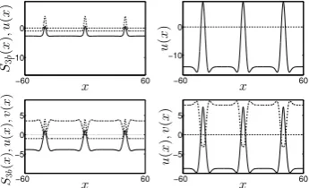
inputs are adjusted in the different examples as indicated in the figure captions. Fig. 1 shows the evolution of a 3-bump solution in response to the three in-puts applied simultaneously at timet= 1. The steady states of the field activity after cessation of the inputs indicate that both models support, in principle, the existence of multiple bumps, and thus, a multi-item working memory. However, the models behave quite differently when the same inputs are presented sequen-tially. As shown in the Fig. 2, the Amari model evolves a single bump whereas the 2-field model again converges to the 3-bump solution. In the Amari case, the steady state excitation pattern in response to the first input (which occupies the permitted total excitation length explained by the theory [1]) creates additional surround inhibition, which ultimately suppresses the initial excitation caused by the subsequent inputs. This is not the case for the 2-field model since the in-creased lateral inhibition in theu-field is compensated by positive feedback from the neurons in thev-field.
−60 60 −10 0 x S3 b ( x ) ,u ( x ) −60 60 −10 0 x u ( x ) −60 60 −5 0 5 x S3 b ( x ) ,u ( x ) ,v ( x ) −60 60 −5 0 5 x u ( x ) , v ( x )
Fig. 1: Left: snapshot of the evolution of a 3-bump solutions at a time when the input distribution S3b(x) (dashed line) is still present. Right: steady state
solutions at time t = 60. Top: activity u(x) (solid line) of the Amari model. Bottom: activities u(x) (solid line) andv(x) (dashed-dotted line) of the 2-field model. Input parameters areSsj = 5 and dsj = 1.
−60 60 0 30 x S1 b ( x ) ,u ( x ) −60 60 0 30 x S1 b ( x ) ,u ( x ) −60 60 0 30 x S1 b ( x ) ,u ( x ) −60 60 0 30 x u ( x ) −60 60 0 15 x S1 b ( x ) ,u ( x ) −60 60 0 15 x S1 b ( x ) ,u ( x ) −60 60 0 15 x S1 b ( x ) ,u ( x ) −60 60 0 15 x u ( x )
Fig. 2: Simulation of the field models with a sequence of three transient inputs
S1b(x) (dashed line). Top: activityu(x) of the Amari model with inputs given by
(5) with Ssj = 25 anddsj = 1. Bottom: activityu(x) of the 2-field model with
inputs given by (5) withSsj = 11 anddsj = 1. The inputs were applied at times
t1= 1 (first column),t2= 17 (second column) andt3= 33 (third column). The
forth column shows the steady state solutions at timet= 60.
[image:6.595.142.478.310.417.2]6 W. Wojtak, S. Coombes, E. Bicho and W. Erlhagen −60 60 0 30 x S1 b ( x ) ,u ( x ) −60 60 0 30 x S1 b ( x ) ,u ( x ) −60 60 0 30 x S1 b ( x ) ,u ( x ) −60 60 0 30 x u ( x ) −60 60 0 40 x S1 b ( x ) ,u ( x ) −60 60 0 40 x S1 b ( x ) ,u ( x ) −60 60 0 40 x S1 b ( x ) ,u ( x ) −60 60 0 40 x u ( x )
Fig. 3: Simulation of the Amari model with a sequence of three transient inputs
S1b(x) (dashed line). In the first row, the inputs were applied at timest1 = 1
(first column),t2= 2 (second column) andt3= 3 (third column). In the second
row, the inputs were applied at times t1 = 1 (first column), t2 = 17 (second
column) and t3 = 33 (third column). Input parameters are Ssj ∈ {5,16,30}
(first row) and Ssj ∈ {5,30,45} (second row) and stimulus duration dsj = 1.
The fourth column shows the steady state solutions at timet= 60.
−60 60 −10 0 10 x u ( x ) 5 15 0 12
Input strength (Ssj)
B u m p a m p li tu d e
β= 0.5
[image:7.595.221.394.336.388.2]β= 1000
Fig. 4: Left: Steady state solution of the 2-field model with a firing rate function given by (2) with steepness parameterβ= 1000. A sequence of three inputs with different strengths Ssj ∈ {5,10,15} and equal duration dsj = 1 was applied.
Right: bump amplitude as a function of the input strength for two steepness parameter values,β = 1000 andβ = 0.5.
−60 60 0 20 x u ( x ) −60 60 0 20 x u ( x )
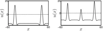
Fig. 5: Steady state solutions of the Amari model (left) and the 2-field model (right) triggered by a sequence of three inputs of different durations dsj ∈ {2.5,1,3}. The inputs are given by (5) withSsj = 25 (left) andSsj = 11 (right),
applied at timestj∈ {1,17,33}.
[image:7.595.221.394.473.525.2]bumps of equal strength (left) is updated by new inputs arriving at later times (right).
−60 60
0 20
x
u
(
x
)
−60 60
0 20
x
u
(
x
[image:8.595.220.396.165.220.2])
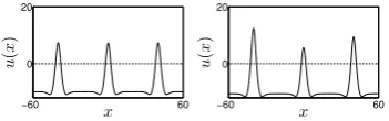
Fig. 6: Left: steady state solution of the 2-field model in response to a sequence of three inputs of equal strength Ssj = 10 presented at timestj ∈ {1,2,3}. Right:
steady state solution of the 2-field model after the presentation of additional inputs at positionxc4 =−40 (with strengthSs4 = 10) and at positionxc5 = 40
(with strengthSs5 = 5). The inputs were applied for a durationdsj = 1 at times
t4= 20 andt5= 22, respectively.
4
Discussion
In this paper we have incorporated a second population into Amari’s one-popula-tion neural field model of lateral inhibione-popula-tion type. The second populaone-popula-tion in-tegrates the activity from the first population with an inverted Mexican-hat connectivity function and projects its activity back locally. We have shown in numerical simulations that the novel field model is able to explain input-selective persistent activity that increases monotonically with the time integral of the in-put. Since the sustained activity is spatially localized, the model combines the defining features of spatial and parametric working memory [15]. Moreover, the model supports a robust temporal integration of behaviorally relevant informa-tion over longer timescales.
Carroll and colleagues [3] have recently proposed a field model that also supports a continuum of possible bump amplitudes. Their model consists of sep-arate excitatory and inhibitory populations that are intra- and interconnected with distance-dependent connectivity functions. However, the parameters of the network and the firing rate function (necessarily of piecewise linear shape) must be tuned precisely (see also [9]). In particular, the recurrent excitation must be inversely proportional to the slope of the nonlinearity to show a monotonic de-pendency of the bump amplitude on input strength. In contrast, the evidence of the present numerical study strongly suggests that the 2-field model is struc-turally stable to changes in model parameters. The lateral inhibition-type cou-pling function of the Amari model is known to support stable bumps over a whole range of parameter values [1,4], and significant changes in the shape of the firing rate function do not disturb parametric working memory (Fig. 4).
8 W. Wojtak, S. Coombes, E. Bicho and W. Erlhagen
model with the behavior of theu-population alone (Amari model). The results show that the feedback from the second population is necessary to ensure a ro-bust formation of a multi-bump solution independent of whether the inputs are presented simultaneously or sequentially.
In future work, we plan to complement the numerical analysis of the novel field model with a more rigorous analysis of bump stability and the dependence of bump amplitude on the integral of the input.
References
1. S. Amari. Dynamics of pattern formation in lateral-inhibition type neural fields.
Biological Cybernetics, 27(2):77–87, 1977.
2. M. Camperi and Xiao-Jing Wang. A model of visuospatial working memory in pre-frontal cortex: recurrent network and cellular bistability. Journal of computational neuroscience, 5(4):383–405, 1998.
3. S. Carroll, K. Josi´c, and Z. P. Kilpatrick. Encoding certainty in bump attractors.
Journal of Computational Neuroscience, pages 1–20, 2013.
4. S. Coombes. Waves, bumps, and patterns in neural field theories. Biological Cy-bernetics, 93(2):91–108, 2005.
5. W. Erlhagen, A. Bastian, D. Jancke, A. Riehle, and G. Sch¨oner. The distribution of neuronal population activation (dpa) as a tool to study interaction and integration in cortical representations. Journal of neuroscience methods, 94(1):53–66, 1999. 6. W. Erlhagen and E. Bicho. The dynamic neural field approach to cognitive
robotics. Journal of Neural Engineering, 3:36–54, 2006.
7. F. Ferreira, W. Erlhagen, and E. Bicho. Multi-bump solutions in a neural field model with external inputs. Physica D: Nonlinear Phenomena, 326:32–51, 2016. 8. I. C. Griffin and A. C. Nobre. Orienting attention to locations in internal
repre-sentations. Cognitive Neuroscience, Journal of, 15(8):1176–1194, 2003.
9. A. A. Koulakov, S. Raghavachari, A. Kepecs, and J. E. Lisman. Model for a robust neural integrator. Nature neuroscience, 5(8):775–782, 2002.
10. C. R. Laing, W. C. Troy, B. Gutkin, and G. B. Ermentrout. Multiple bumps in a neuronal model of working memory. SIAM Journal on Applied Mathematics, 63(1):62–97, 2002.
11. E. K. Miller. The prefontral cortex and cognitive control. Nature reviews neuro-science, 1(1):59–65, 2000.
12. R. Romo, C. D. Brody, A. Hern´andez, and L. Lemus. Neuronal correlates of parametric working memory in the prefrontal cortex. Nature, 399(6735):470–473, 1999.
13. E. Salinas. How behavioral constraints may determine optimal sensory represen-tations. PLoS Biol, 4(12):e387, 2006.
14. A. R. Schutte, J. P. Spencer, and Gregor Sch¨oner. Testing the dynamic field theory: Working memory for locations becomes more spatially precise over development.
Child development, 74(5):1393–1417, 2003.
15. Xiao-Jing Wang. Synaptic reverberation underlying mnemonic persistent activity.
Trends in neurosciences, 24(8):455–463, 2001.