Advance Access publication 2013 December 5
Classical T Tauri stars: magnetic fields, coronae and star–disc interactions
C. P. Johnstone,
1‹M. Jardine,
2S. G. Gregory,
2J.-F. Donati
3and G. Hussain
41University of Vienna, Department of Astrophysics, T¨urkenschanzstrasse 17, A-1180 Vienna, Austria 2School of Physics and Astronomy, Universtiy of St Andrews, St Andrews, KY16 9SS, UK
3LATT-UMR 5572, CNRS & Univ. P. Sabatier, 14 Av. E. Belin, F-31400 Toulouse, France 4ESO, Karl-Schwarzchild-Str. 2, D-85748 Garching, Germany
Accepted 2013 October 30. Received 2013 October 29; in original form 2013 July 10
A B S T R A C T
The magnetic fields of young stars set their coronal properties and control their spin evolution via the star–disc interaction and outflows. Using 14 magnetic maps of 10 classical T Tauri stars (CTTSs) we investigate their closed X-ray emitting coronae, their open wind-bearing magnetic fields and the geometry of magnetospheric accretion flows. The magnetic fields of all the CTTSs are multipolar. Stars with simpler (more dipolar) large-scale magnetic fields have stronger fields, are slower rotators and have larger X-ray emitting coronae compared to stars with more complex large-scale magnetic fields. The field complexity controls the distribution of open and closed field regions across the stellar surface, and strongly influences the location and shapes of accretion hot spots. However, the higher order field components are of secondary importance in determining the total unsigned open magnetic flux, which depends mainly on the strength of the dipole component and the stellar surface area. Likewise, the dipole component alone provides an adequate approximation of the disc truncation radius. For some stars, the pressure of the hot coronal plasma dominates the stellar magnetic pressure and forces open the closed field inside the disc truncation radius. This is significant as accretion models generally assume that the magnetic field has a closed geometry out to the inner disc edge.
Key words: stars: activity – circumstellar matter – stars: coronae – stars: magnetic field – stars: pre-main sequence – stars: rotation – stars: variables: T Tauri, Herbig Ae/Be.
1 I N T R O D U C T I O N
T Tauri stars are low-mass, pre-main-sequence (PMS) stars char-acterized by large irregular variability and the presence of strong
emission lines (Edwards et al.1994; Ardila et al.2013). They are
classified as either classical T Tauri stars (CTTSs) or weak-line T Tauri stars (WTTSs). CTTSs show excess IR emission from circum-stellar discs, and excess UV and optical emission from the accretion of disc material. WTTSs are in a more evolved state where they have lost their discs and are no longer accreting.
CTTSs host strong magnetic fields with measured surface
aver-aged strengths of up to a few kG (Johns-Krull2007). These fields are
responsible for several processes on CTTSs, such as X-ray emission from magnetically confined coronae, the truncation of circumstellar discs several stellar radii from the star, and magnetospheric accre-tion. In order to study these processes, surface averaged magnetic field strengths are not sufficient and it is necessary to know about the topologies of the large-scale magnetic fields of these stars. This is
E-mail:[email protected]
done using the Zeeman–Doppler Imaging (ZDI) technique, which uses time-resolved spectropolarimetric observations of stars over several rotations to reconstruct the distributions and orientations
of the large-scale magnetic fields over their surfaces (Semel1989;
Donati2001).
ZDI magnetic maps have recently been published for a sample of CTTSs with different masses and ages as part of the Magnetic
Pro-tostars and Planets project (Donati et al.2010a) and have shown that
CTTSs possess magnetic fields with a range of strengths and topolo-gies. The topologies range from simple, almost axisymmetric fields on AA Tau and BP Tau, to much more complex non-axisymmetric fields on CR Cha, CV Cha and V2247 Oph. The strengths and topologies of these fields appear to be related to the internal
struc-tures of the host stars (Gregory et al.2012). Stars that are yet to
develop radiative cores (e.g. AA Tau and BP Tau) possess strong simple axisymmetric fields dominated by low-order spherical har-monic components. Stars that are no longer fully convective possess much weaker and more complex non-axisymmetric fields. The ex-ception is V2247 Oph, which possesses a highly complex and weak field but has too low a mass to develop a radiative core as it evolves.
These results have been reviewed by Gregory & Donati (2011) and
C
2013 The Authors Published by Oxford University Press on behalf of the Royal Astronomical Society
at Library & Information Services, University of St Andrews on January 13, 2014
http://mnras.oxfordjournals.org/
Hussain (2012). Similar results have been found for the sample of main-sequence M dwarfs that have been studied using ZDI (Donati
et al.2008b; Morin et al.2008,2010), though for PMS stars, the
situation is more complicated because the internal structure of PMS
stars is determined by both mass and age (Gregory et al.2012).
T Tauri stars show very high levels of X-ray emission, with
typical X-ray luminosities of 1028–1032 erg s−1(Walter & Kuhi
1981; Preibisch et al.2005). In most cases, the majority of X-ray
emission comes from hot magnetically confined coronae (Stassun
et al.2006). Whereas the solar corona is at temperatures of a few
MK, the coronae of T Tauri stars can be up to 50 MK (Preibisch et al.
2005; G¨udel et al.2007). X-ray emission from CTTSs also comes
from large stellar flares (e.g. Getman et al.2008), X-ray jets (e.g.
G¨udel et al.2008) and accretion shocks where material accreting
from the disc impacts the stellar surface at supersonic speeds (e.g.
Argiroffi et al.2011). The most extreme example of X-ray emission
from an accretion shock is the case of TW Hya. TW Hya is viewed almost pole-on, which makes it ideal for observing emission from accretion shock regions. Analysis of TW Hya’s X-ray spectrum has indicated that the star’s X-ray emission measure is dominated by a low-temperature, high-density plasma, most likely formed in
accretion shocks (Kastner et al.2002; Robrade & Schmitt 2006;
Brickhouse et al.2010).
Early disc and accretion models assumed that discs extend all the way to the stellar surface and accretion occurs through a
bound-ary layer (e.g. Lynden-Bell & Pringle1974). However, the strong
magnetic fields of CTTSs are able to truncate the disc far from the stellar surface and funnel accretion along magnetic field lines at
approximately free-fall velocities – typically a few hundred km s−1
– on to the stellar surface. This model was originally developed for
magnetic neutron stars (Ghosh, Pethick & Lamb1977; Ghosh &
Lamb1979a,b) and applied to CTTSs by Camenzind (1990) and
K¨onigl (1991). When accreting material impacts the stellar surface,
accretion shocks are formed. The post-shock plasma has densities
of 1012–1013cm−3and temperatures of a few MK (Argiroffi et al.
2011). These shocks account for the excess UV and optical emission
from CTTSs (K¨onigl1991), and are also responsible for significant
amounts of softer X-ray emission.
By making assumptions about the magnetic fields, 2D surface magnetic maps can be used to reconstruct the 3D coronal field geometries. These extrapolations can be used to estimate the
struc-ture of the X-ray emitting closed corona. Jardine et al. (2002) used
potential field extrapolations of the young rapidly rotating main-sequence star AB Dor to infer the global X-ray emission measure and rotational modulation. They found that a magnetically confined isothermal corona in hydrostatic equilibrium could give the ob-served emission measures with average coronal electron densities
of 109.0–1010.7cm−3. Jardine et al. (2006) used a similar model to
show how the differences between the coronal properties of stars are related to their magnetic field geometries. They found that stars with complex magnetic fields tend to have coronal plasma densities that are of an order of magnitude higher than stars with simple dipolar geometries. They also found that the observed correlation between
X-ray emission and stellar mass (Preibisch et al.2005; G¨udel et al.
2007) can arise from variations in the surface gravities and the sizes
of the closed coronae.
These field extrapolations are also useful for studying magne-tospheric accretion on to CTTSs. Most accretion models assume that the stellar magnetic field is an axisymmetric dipole. However, recent studies using ZDI have shown that CTTSs often have much more complex field structures. For an axisymmetric dipole field, accretion footpoints can be expected to be seen distributed in bands
around the star. However, if the dipole component is tilted with respect to the star’s rotation axis, these bands no longer extend all the way around the star, and cover a smaller fraction of the stellar
surface (Mahdavi & Kenyon1998; Romanova et al.2003,2004;
Gregory et al.2006). Gregory et al. (2006) used field extrapolations
of surface fields for real stars to model accretion on to stars with complex magnetic fields. For such fields, accretion hotspots can be distributed over the stellar surface in highly complex patterns. Sim-ilar results were found using ZDI magnetic maps from BP Tau and
V2129 Oph by Gregory et al. (2008) and Jardine, Gregory & Donati
(2008), and using 3D magnetohydrodynamic (MHD) simulations
by Long et al. (2011) and Romanova et al. (2011). They found that
the latitudes at which accreting material impacts the stellar surface is determined by the distance from the star that the disc is trun-cated, with large disc truncation radii leading to accretion located at high latitudes and small disc truncation radii leading to accretion footpoints distributed over a range of latitudes.
In this paper, we analyse the magnetic fields of the sample of CTTSs with published ZDI magnetic maps and use field extrapo-lations to study the closed X-ray emitting coronae, and accretion
geometries on these stars. This is similar to Lang et al. (2012) who
used similar models to investigate the field structures and coronal X-ray emission on the sample of M dwarf main-sequence stars with published ZDI maps. In Section 2, we discuss the stars in the sam-ple; in Section 3, we analyse the ZDI magnetic maps for these stars; in Section 4, we model their closed X-ray emitting coronae; in Sec-tion 5, we calculate disc truncaSec-tion radii, and accreSec-tion geometries, for these stars; and in Section 6, we summarize the results, and discuss our conclusions.
2 T H E S A M P L E
In this paper, we use the published magnetic maps for the CTTSs
AA Tau (Donati et al.2010a), BP Tau (Donati et al.2008a), CR
Cha (Hussain et al.2009), CV Cha (Hussain et al.2009), GQ Lup
(Donati et al.2012), TW Hya (Donati et al.2011b), V2129 Oph
(Donati et al.2007,2011a), V2247 Oph (Donati et al.2010b), and
both stars in the binary system V4046 Sgr (Donati et al.2011c).
The original magnetic maps for CR Cha and CV Cha, published
by Hussain et al. (2009), were produced using a different fitting
technique than was used to produce the other maps; therefore, we do not use these maps. Instead, we use new maps produced using the same observational data but with an updated ZDI code that fits the maps directly to the circularly polarized line profiles as a series of spherical harmonic components, which is the technique used to fit the maps for the other stars. These maps can be seen
in Fig.1. Another difference between the fitting method used for
the CR Cha and CV Cha maps and the fitting method used for the other stars is the fact that Zeeman signatures from accretion proxies were used to fit the magnetic maps of the other stars, but were not used for CR Cha and CV Cha because no Zeeman signatures were detected in accretion related emission lines for these stars. This could potentially remove magnetic energy from the axisymmetric spherical harmonic components of the field, and move magnetic
energy to higherl-value modes. The effects of not including the
accretion related emission lines in ZDI fits were explored by Donati
et al. (2007) for the case of V2129 Oph.
The stellar parameters for these stars are summarized in Table1
and the published magnetic maps for AA Tau and V2247 Oph
are shown in Fig.1. Detailed discussions of the adopted stellar
parameters for each star can be found in the papers (listed above) where the magnetic maps have been published. As mass accretion
at Library & Information Services, University of St Andrews on January 13, 2014
http://mnras.oxfordjournals.org/
Figure 1. The radial components of the ZDI magnetic maps for AA Tau (Donati et al.2010a), V2247 Oph (Donati et al.2010b), CR Cha and CV Cha. We show the AA Tau and V2247 Oph maps because they are the most simple and the most complex large-scale magnetic fields in the sample; we show the CR Cha and CV Cha maps because they have not previously been published.
Table 1. Stellar parameters from the literature for all of the stars in the sample. The stars are ordered from top to bottom alphabetically. From left to right, the columns correspond to stellar mass, stellar radius, rotation period, age, corotation radius, projected rotational velocity, mass accretion rate, coronal temperature and coronal X-ray emission measure. References for each value are given as superscripts and correspond to the following papers: 1. Donati et al. (2010a); 2. Vrba et al. (1989); 3. Bouvier et al. (2007); 4. Hartmann & Stauffer (1989); 5. Nguyen et al. (2009); 6. G¨udel et al. (2007); 7. Johns-Krull, Valenti & Koresko (1999); 8. Donati et al. (2008a); 9. Vrba et al. (1986); 10. Donati et al. (2010b); 11. Robrade & Schmitt (2006); 12. Hussain et al. (2009); 13. Bouvier et al. (1986); 14. Nguyen et al. (2009); 15. Weise et al. (2010); 16. Stempels & Piskunov (2003); 17. Donati et al. (2012); 18. Donati et al. (2011b); 19. Hu´elamo et al. (2008); 20. Torres et al. (2003); 21. Donati et al. (2011a); 22. Grankin et al. (2008); 23. Donati et al. (2007); 24. Argiroffi et al. (2011); 25. Pillitteri et al. (2010); and 26. Donati et al. (2011c).
Star M R Prot Age Rco vsini log ˙Ma logT(K) log EM
(M) (R) (d) (Myr) (R) (km s−1) (M
yr−1) (K) (cm−3) AA Tau 0.701 2.001 8.202, 3 1.51 7.6 12.34, 5 −9.21 7.436 52.956 BP Tau 0.707 1.958 7.609 1.58 6.0 9.07, 8 −8.610 7.0611 53.2811 CR Cha 1.9012 2.5012 2.3013 3.012 3.6 35.014, 15 −9.012 7.1011 53.4011
CV Cha 2.0012 2.5012 4.4013 5.012 5.7 25.016 −7.512 – –
GQ Lup 1.0517 1.7017 8.4017 2.0-5.017 10.4 5.017 −9.017 – – TW Hya 0.8018 1.1018 3.5619 8.018 8.3 5.015, 20 −8.918 7.1111 52.6411 V2129 Oph 1.3521 2.0021 6.5322 2.321 8.1 14.515, 23 −9.221 7.0524 53.5924 V2247 Oph 0.3610 2.0010 3.5022 1.010 3.4 20.513 −9.810 7.1825 53.0825 V4046 Sgr A 0.9526 1.1226 2.4226 15.026 2.5 13.526 −9.326 – – V4046 Sgr B 0.8526 1.0426 2.4226 15.026 2.7 12.526 −9.326 – –
can be highly variable in time, in all cases we use mass accretion rates derived from the same observations as the ZDI maps. The lowest mass star in the sample is V2247 Oph, which has a mass
of 0.36 M and is therefore unlikely to develop a radiative core
at any age. Other than AA Tau and BP Tau, which are both still fully convective, the other stars in the sample all host radiative cores.
For the coronal models in Section 4, we require coronal temper-atures and X-ray emission measures for each of the stars. We take from the literature multitemperature component fits to the observed
X-ray spectra (for references, see Table1). For most of these stars,
these fits have low-temperature components that we assume are a result of accretion shocks; we therefore disregard these compo-nents. As our model assumes an isothermal corona, we combine the
at Library & Information Services, University of St Andrews on January 13, 2014
http://mnras.oxfordjournals.org/
[image:3.595.106.485.494.631.2]remaining components to get the coronal temperature and emission measure using
EM=
i
EMi (1)
and
logT =
iEMilogTi
iEMi .
(2)
For AA Tau, the components in the fit to the X-ray spectrum by
G¨udel et al. (2007) are all above 10 MK, and are therefore unlikely
to have been produced in accretion shocks; we therefore assume that all of these components correspond entirely to coronal emis-sion. For BP Tau and CR Cha, the three temperature component
fits given by Robrade & Schmitt (2006) both have low-temperature
components at approximately 2 MK, which could be a result of X-ray emission from accretion shocks; we therefore disregard these components. However, these components are only 18 per cent of the total emission measures, so this only makes a small difference to the coronal models. Similarly, for V2129 Oph, we disregard the three lowest temperature components of the nine-temperature
com-ponent emission measure distribution fit of Argiroffi et al. (2011);
these components only correspond to 8 per cent of the total emission measure. For V2247 Oph, the low-temperature component of the
three-temperature component fit given by Pillitteri et al. (2010) has
an emission measure that is comparable to the high-temperature components. For TW Hya, the X-ray emission measure is
domi-nated by a low-temperature, high-density plasma at∼3 MK which
probably corresponds to an accretion shock (Kastner et al.2002;
Stelzer & Schmitt2004; Brickhouse et al.2010). We use the
three-temperature component fit given by Robrade & Schmitt (2006) and
we disregard the low-temperature component. This may have a sig-nificant effect on the coronal model. No temperature and emission measure fits are available for CV Cha and GQ Lup.
3 S U R FAC E F I E L D S
In this section, we analyse the available sample of ZDI maps. Al-though most of these fields were fitted as the sum of poloidal and
toroidal components,1for the extrapolations that we use in this paper
we assume that the fields are potential, and we therefore disregard the toroidal components of the fields. We are therefore left with
only theBr(θ,φ) components of the ZDI fits as these are described
entirely by the poloidal components. TheBθ(θ,φ) andBφ(θ,φ)
components are then reconstructed fromBr(θ,φ) based on the
po-tential field model, which we describe in more detail in Section 4.1. In this model, the field is described as an expansion of spherical harmonic multipoles. For instance, at the stellar surface, the radial component of the field is given by
Br(θ, φ)= ∞
l=1 l
m=−l
clmPlm(cosθ)eimφ, (3)
wherePlm(cosθ) are the associated Legendre polynomials,θis the
colatitude (with values of 0 andπat the poles of the coordinate
system),φis the longitude andclmcharacterizes the strengths of the
1It is common in the literature to define the poloidal component of a mag-netic field as a combination of theBrandBθcomponents, and the toroidal component as theBφ components. Within the ZDI community, the defi-nitions of these terms are different and are described in appendix III of Chandrasekhar (1961).
spherical harmonic components. In this model, thel=1 components
represent dipole fields, thel=2 components represent quadrupole
fields and thel=3 components represent octupole fields. In general,
higherlvalues represent more complex fields.
It is useful to have a simple way to quantify how magnetic en-ergy is distributed between high- and low-order spherical harmonic
components.2For this, we use the energy-weighted averagelvalue
that describes the field. This is given by
l = ∞
l=1Ell
∞
l=1El
, (4)
whereElis the magnetic energy held within eachl-value
compo-nent. We compute this quantity using only the poloidal component of the field so that the results can be compared to the field
extrapola-tions in the following secextrapola-tions. Since the strengths of higherl-value
components decreases with distance from the star faster than the
strengths of lowerl-value components, this is a simple measure of
the rate at which the star’s magnetic field strength falls off with distance from the star (see Section 4). This can also be thought of as a simple measure of the complexity of a magnetic field because
fields with simple dipolar configurations have low values of l,
and fields with lots of small-scale features have higher values of
l. However, this does not take into account the amount of
mag-netic energy in non-axisymmetric spherical harmonic components, which can be considered when constructing a more representative measure of field complexity.
3.1 Results
The radial components of the previously published magnetic maps for AA Tau and V2247 Oph, and the new maps for CR Cha and
CV Cha are shown in Fig.1. There is significant variation in
mag-netic field complexity across all of the magnetograms in the sample. Some stars have large-scale fields that are well described with dipole plus octupole components, namely, in increasing/decreasing impor-tance of the octupole/dipole component, AA Tau, BP Tau, GQ Lup, V2129 Oph and TW Hya. The other stars, V2247 Oph, CR Cha, CV Cha, V4046 Sgr A and V4046 Sgr B, have more complex field
topologies. In Table2, we give the total unsigned magnetic fluxes,
surface averaged field strengths,lvalues, and the strengths of the
dipole and octupole components for each of the fields. We define the strength of the dipole component as the polar field strength of the dipole component (i.e. the polar field strength of a field that con-sists of the dipole component only), and we use a similar definition for the strength of the octupole component. The strengths of the dipole components are important as these components dominate far from the star and therefore primarily determine the open magnetic fluxes and disc truncation radii. The octupole components are im-portant because ZDI studies suggest that CTTSs often possess very strong octupole components. As we do not consider the toroidal components of the fields, the surface averaged field strengths are underestimates for the true values derived from the ZDI fits.
The simplest large-scale field in the sample is on the fully convec-tive star AA Tau, which has a strong dipole component of strength
2We define the magnetic energy as the magnetic energy density,B2, inte-grated over the stellar surface. Although this does not actually give energy, if we integrate this outwards in radius by a small distance, the magnetic field can be assumed to be uniform over this distance. Since we only ever consider the energy in each spherical harmonic component as the fraction of the total energy in the field, this integral outwards in radius can be ignored.
at Library & Information Services, University of St Andrews on January 13, 2014
http://mnras.oxfordjournals.org/
Table 2. Results for the analysis of the ZDI magnetic maps for all of the stars in the sample. The maps are arranged from top to bottom by decreasing strength of the dipole component of the field. From left to right, the columns correspond to the total unsigned magnetic flux, the surface field strength averaged over the stellar surface, the strength of the dipole component, the strength of the octupole component, the tilt angle of the dipole component relative to the rotation axis and the parameterldefined as the energy-weighted average lvalue that describes the field. The parameterlcan be used as a measure of the rate at which the magnetic field strength decreases with increasing distance from the star, and can also be used as a proxy for field complexity. For BP Tau, the magnetic maps used here were produced using an experimental version of the ZDI code. However, analysis conducted with a more advanced version of the code has produced similar results (see footnote 1 of Gregory & Donati2011).
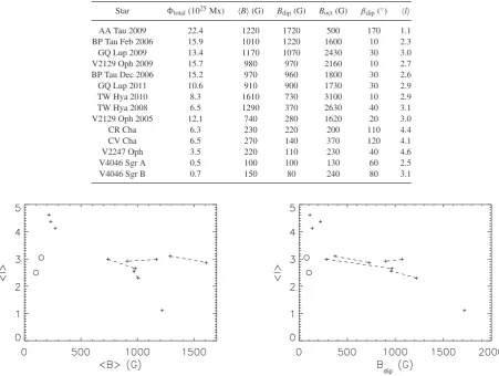
Star total(1025Mx) B(G) Bdip(G) Boct(G) βdip(◦) l
AA Tau 2009 22.4 1220 1720 500 170 1.1
BP Tau Feb 2006 15.9 1010 1220 1600 10 2.3
GQ Lup 2009 13.4 1170 1070 2430 30 3.0
V2129 Oph 2009 15.7 980 970 2160 10 2.7
BP Tau Dec 2006 15.2 970 960 1800 30 2.6
GQ Lup 2011 10.6 910 900 1730 30 2.9
TW Hya 2010 8.3 1610 730 3100 10 2.9
TW Hya 2008 6.5 1290 370 2630 40 3.1
V2129 Oph 2005 12.1 740 280 1620 20 3.0
CR Cha 6.3 230 220 200 110 4.4
CV Cha 6.5 270 140 370 120 4.1
V2247 Oph 3.5 220 110 230 40 4.6
V4046 Sgr A 0.5 100 100 130 60 2.5
V4046 Sgr B 0.7 150 80 240 80 3.1
Figure 2. Left-hand panel: correlation betweenland the surface averaged field strengthBfor the sample of ZDI magnetic maps. Right-hand panel: correlation betweenland the strength of the dipole component of the field. The two stars in the binary system V4046 Sgr are shown as open circles. Data points representing the same star from two different epochs are connected by dashed lines.
1.7 kG and an octupole component of strength 500 G. The field has
anlvalue of 1.1, which means that almost all of the magnetic
energy is held in the dipole component of the field. The stars BP Tau, GQ Lup, TW Hya, V2129 Oph, V4046 Sgr A and V4046 Sgr B
also possess simple large-scale fields, withlvalues of∼2–3. In
each case, the octupole component has a much stronger polar field strength than the dipole component. For the two BP Tau fields, and the V2129 Oph 2009 field, the dipole and octupole components have equal strengths at low latitudes. For the two TW Hya fields, and the V2129 Oph 2005 field, the octupole component dominates
at all latitudes. Due to the strong∼3 kG octupole component on
TW Hya, this field has the largest value of the surface averaged field strength. Due to its relatively old age, TW Hya has a relatively small surface area; this means that it has a much smaller unsigned
mag-netic flux. All of these fields have surface averaged field strengths above 500 G.
The magnetic fields on CR Cha, CV Cha and V2247 Oph, have
largerlvalues between 4 and 5. For V2247 Oph, the polar regions
show single polarity fields, and the low-latitude fields are covered in complex patterns of regions of opposite polarity field. For CR Cha and CV Cha, the complex patterns of regions of opposite polarity field cover the stellar surfaces at all latitudes. All of these stars have very weak large-scale fields, with surface averaged field strengths of a few hundred Gauss.
In Fig.2, we show that there is some correlation betweenland
B. The simple fields are the strongest, and the more complex fields
are the weakest. The possible exceptions are the fields on V4046 Sgr A and V4046 Sgr B, which appear to have relatively weak fields
at Library & Information Services, University of St Andrews on January 13, 2014
http://mnras.oxfordjournals.org/
given their small values ofl. A similar correlation between field strength and field complexity is seen on the M dwarfs that have been
studied using ZDI (Donati et al.2008b; Morin et al.2008,2010).
Since the spatial resolution of the ZDI technique is dependent on stellar rotation rate – the fastest rotators have the highest resolution – it is important to understand to what extent the differences in the complexities of the ZDI maps are resolution effects. Hussain et al.
(2009) explored this possibility for CR Cha, CV Cha, BP Tau and
V2129 Oph. These stars have projected rotational velocities of 35,
25, 9 and 14.5 km s−1, respectively. They produced simulated data
for CR Cha and CV Cha based on the reconstructed magnetic maps for the two stars, and assuming the stellar parameters of BP Tau and V2129 Oph. Using these simulated data, they again reconstructed the magnetic topologies for CR Cha and CV Cha. They found that the stellar parameters of V2129 Oph gave magnetic maps for CR Cha and CV Cha of similar complexity to the magnetic map of
V2129 Ophbut with much smaller field strengths. However, when
they assumed the BP Tau parameters, their reconstructed fields were significantly more complex than the field found on BP Tau. This indicates that the large-scale magnetic field of BP Tau is genuinely much simpler than those of CR Cha, CV Cha and V2129 Oph; if BP Tau hosted a more complex large-scale field, then it would have been detected by ZDI.
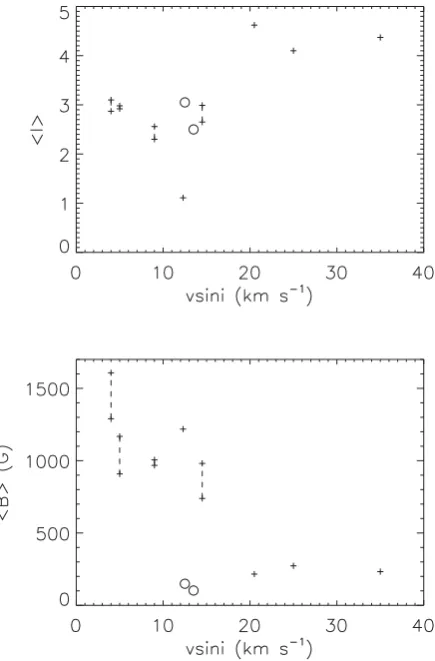
In Fig.3, we show a clear correlation betweenland projected
rotational velocity. Although this is consistent with the
[image:6.595.317.539.57.211.2]interpreta-Figure 3. Upper panel: correlation between the projected rotational velocity andl. Lower panel: correlation between the projected rotational velocity and the surface averaged field strength. The two stars in the binary system V4046 Sgr are shown as open circles. Data points representing the same star from two different epochs are connected by dashed lines.
Figure 4. Correlation between the strength of the dipole component of the field and the stellar rotation period. Stars with weak dipole components tend to be rotating faster than stars with strong dipole components. The two stars in the binary system V4046 Sgr are shown as open circles. Data points representing the same star from two different epochs are connected by dashed lines.
tion that the differences between the complexities of the magnetic maps is a resolution effect since greater field complexity can only be recovered on faster rotators, if this interpretation was correct, we would expect that the strongest field strengths would be seen on the rapid rotators due to a lower amount of flux cancellation. However,
these stars show the opposite trend, as we show in Fig.3. Also,
in the sample of M dwarfs with known large-scale fields geome-tries, reconstructed using the same ZDI technique, there is no clear correlation between field complexity and rotation rate. In fact, in many cases, the rapidly rotating main-sequence M dwarfs have the simplest fields.
The correlation betweenl, field strength and rotation rate may
be a result of star–disc magnetic interactions. Coupling between the stellar magnetic field and the disc leads to torques being exerted on the central star. Magnetic field lines extending from the star to regions of the disc inside the corotation radius exert a spin-up torque on the star; magnetic field lines extending from the star to regions of the disc beyond the corotation radius exert a spin-down torque on the star. Stars with stronger dipole fields might be expected to rotate slower for two reasons. First, a stronger dipole field will truncate the inner edge of the disc further from the stellar surface, which might lead to a smaller spin-up torque on the central star. At the same time, a stronger dipole field will couple to the disc beyond the corotation radius more efficiently, leading to a greater spin-down torque. Thus, the correlation between rotation rate and the
strength of the dipole component, seen in Fig.4, could be a natural
consequence of star–disc interactions. As the strength of the dipole component is positively correlated with the field complexity and the average field strength, this can explain why the faster rotators have stronger and more complex fields.
4 C L O S E D X - R AY E M I T T I N G C O R O N A E
4.1 Model
Based on the solar analogy, we model the coronal magnetic fields of the CTTSs as potential fields (meaning that they contain no electric currents) using the potential-field source-surface (PFSS) model. Although stellar closed coronae contain hot plasma that alters the magnetic field structures, in the Sun, the PFSS model is reasonably
at Library & Information Services, University of St Andrews on January 13, 2014
http://mnras.oxfordjournals.org/
[image:6.595.59.277.344.675.2]accurate when describing large-scale magnetic field geometries. This has been shown by comparisons of closed coronal structures predicted with the PFSS model with images of the green line solar
corona (Wang et al.1997) and by comparisons of the PFSS model
with the results of MHD modelling for the solar corona (Riley et al.
2006) and for other stars (Jardine et al. 2013). Although in the
large-scale corona, we do not expect currents to significantly alter the magnetic field structure, on small scales, the field structures will be significantly altered by subsurface convective motions. Since we do not model small-scale field structures, this issue is not considered in this paper. It is unclear to what extent large stellar flares affect coronal magnetic field structures, and such effects are not included in our models. Our models therefore correspond to quiescent (non-flaring) coronae.
Assuming the magnetic field is potential (current free) means that it can be described entirely by the gradient of a magnetostatic
scalar potential, whereB= −∇. In this case,must satisfy
Laplace’s equation∇2=0, the solution of which can be written
as a spherical harmonic expansion:
(r, θ, φ)= ∞
l=1 l
m=−l
almrl+blmr−(l+1)Plm
(cosθ)eimφ. (5)
If the field strength is assumed to vanish very far from the star, then
the values ofalmmust all be zero. However, the coronal magnetic
field structures that are consistent with this assumption are unreal-istic because they do not take into account the opening of magnetic field lines by coronal plasma. This happens approximately at the
point where the plasmaβbecomes greater than unity, and the field
lines beyond that point are approximately radial. This can be cor-rected for in the potential-field model by assuming a spherical source
surface with radiusRSwhere the field becomes entirely radial, i.e.
Bθ(RS)=Bφ(RS)=0. Making the source-surface assumption, and
definingclm=blm(l+1)R−(l+2)−almlRl−1, gives
Br(r, θ, φ)= ∞
l=1 l
m=−l
clmfl(r)Plm(cosθ)eimφ (6)
Bθ(r, θ, φ)= ∞
l=1 l
m=−l
clmgl(r)dPlm(cosθ)
dθ e
imφ (7)
Bφ(r, θ, φ)= ∞
l=1 l
m=−l
clmgl(r)Plm(cosθ) im
sinθe
imφ, (8)
wherefl(r) andgl(r) are given by
fl(r)=
⎡ ⎢ ⎣(l+1)
r R
−(l+2)
+l RS R
−(2l+1) r R
l−1
l RS R
−(2l+1)
+l+1
⎤ ⎥
⎦ (9)
gl(r)=
⎡ ⎢ ⎣
r R
l−1 RS R
−(2l+1)
− r R
−(l+2)
l RS R
−(2l+1)
+l+1
⎤ ⎥
⎦. (10)
This is the PFSS model, developed by Altschuler & Newkirk (1969)
and Schatten, Wilcox & Ness (1969), and is discussed in detail
by Gregory et al. (2010) and Johnstone (2012). When the
source-surface radius is very large, this is equivalent to taking alm =0
in equation (5). At the stellar surface,fl(r)=1, and equation (6)
reduces to equation (3). The values of theclmcoefficients are
calcu-lated using only the radial components of the ZDI maps. This means
that the non-potential components of the ZDI maps are not taken
into account in the extrapolations. Jardine et al. (2013) used MHD
stellar wind models to investigate the effects that ignoring toroidal fields can have on field extrapolations and found that the presence of toroidal surface fields is incompatible with a wind solution that is in force balance, and therefore such fields must be confined close to the stellar surface, below the heights at which the wind is launched. The code that we use to extrapolate the fields was originally developed
by van Ballegooijen, Cartledge & Priest (1998). The free parameter
in this model is the source-surface radius,RS, which we set to the
equatorial corotation radius. At this radius, the exact choice of the source-surface radius is unlikely to have a significant effect on the
coronal plasma model (Jardine et al.2008).
Using the field extrapolations, we model the closed coronal plasma by assuming an isothermal corona in hydrostatic equilib-rium that is corotating with the stellar surface. This model has been
developed by Jardine et al. (2002,2006,2008). The isothermal and
hydrostatic equilibrium assumptions mean that the plasma pressure along each magnetic loop is given by
p=p0exp
¯ m kT
gsds
, (11)
wherep0is the plasma pressure at the base of each field line, ¯mis
the mean molecular mass,sis the coordinate measured along the
path of the magnetic loop, andgsis the component of the effective
gravity parallel to the field line. This is given by
gs= g.B
|B|, (12)
where
g(r, θ)=−GM/r2+ω2rsin2θ, ω2rsinθcosθ. (13)
HereMis the stellar mass,ris the distance from the centre of the
star,ωis the stellar surface angular velocity (we ignore differential
rotation) andθis the colatitude coordinate. Although the opening of
coronal field lines is simulated using the source-surface assumption in the field extrapolation model, we further apply the condition that the density is zero at any point if the field line through that point has a gas pressure that exceeds the magnetic pressure anywhere along its length. Such field lines are assumed to be dark in X-rays and do not contribute to the X-ray emission measure.
We assume that the plasma pressure at the base of the corona,p0,
is proportional to the magnetic pressure, such that
p0=KB02, (14)
whereB0is the average of the magnetic field strengths at the two
footpoints of the magnetic loop. This ensures that regions of strong magnetic field give the highest densities and is similar to the model
of Wang et al. (1997). They modelled the solar corona using field
extrapolations of synodic magnetograms and fitted their model to simultaneous green light observations of the corona. We assume
thatKis uniform over the surface of each star, but varies from star
to star. In order for there to be a closed corona, the value ofKmust
be significantly less than unity. For each star, we scaleKsuch that
the modelled global emission measures (i.e.n2
eintegrated over the
closed coronal volume) fit the observed X-ray emission measures from the literature. The coronal temperatures and emission measures compiled from the literature for each star are discussed in Section 2. As no coronal temperatures and emission measures are available for CV Cha and GQ Lup in the literature, we do not consider them in this section. We also do not consider the two stars in the close
at Library & Information Services, University of St Andrews on January 13, 2014
http://mnras.oxfordjournals.org/
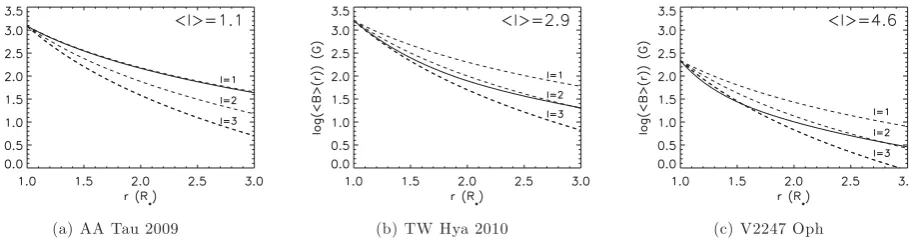
Figure 5. Shows magnetic field strengths, averaged over all latitude and longitude, as a function of distance from the star for the field extrapolations (with no source surface assumed) of AA Tau, TW Hya 2010 and V2247 Oph. The magnetic fields of AA Tau, TW Hya 2010 and V2247 Oph are good examples of dipole fields, octupole fields and more complex fields, respectively, and the 3D potential field extrapolations of these magnetic fields can be seen in Fig.11. The corresponding field strengths, as functions of radius, for dipole (l=1), quadrupole (l=2) and octupole (l=3) fields with the same surface field strengths are shown as dashed lines. This shows how fast the strengths of magnetic fields of different complexities decrease with increasing radius. The decrease in the steepness of the slopes with increasing radius for both TW Hya 2010 and V2247 Oph, shows how the influence of high-order spherical harmonic components diminishes far from the stellar surface. Close to the stellar surfaces of TW Hya and V2247 Oph, the field strengths decrease with increasing radius faster than for the more dipolar field of AA Tau. However, further from the star, the field strengths decrease with radius at the same rate as the AA Tau field. Despite the different field complexities, in all three cases, the field strength falls off far from the star at the same rate as a dipole (B∝r−3). This is due to the dominance of the dipole component far from the stellar surface.
binary system V4046 Sgr as the nature of the system is much more complex than the others in the sample.
Due to the reliance of the ZDI technique on Stokes V (circularly polarized) line profiles, ZDI magnetic maps suffer from missing
magnetic flux in small-scale field structures. Reiners (2011)
com-pared surface magnetic fluxes measured using Stokes I and Stokes V for a number of M dwarf main-sequence stars, and found that
Stokes V typically reproduced only∼5 per cent of the magnetic
flux found using Stokes I. This missing flux is probably contained within small-scale active regions similar to those found on the
so-lar surface. Johnstone, Jardine & Mackay (2010) and Arzoumanian
et al. (2011) investigated the effects of missing magnetic flux on
the coronal models used in this paper. They found that when mag-netic maps are dominated by small-scale field structures, the coronal X-ray emission is dominated by these field structures. Therefore, the possibility that large amounts of magnetic flux are missing on small scales in the ZDI magnetic maps represents a limitation to our models. Nevertheless, the magnetic maps that we use in this paper represent the highest quality data available from current instrumen-tation. In Appendix A, we test the effects of missing small-scale field structures on the results presented in this section. The loss of small-scale field structures is important mostly due to the effect on
theKparameter in the model, which we fit to observationally
con-strained emission measures. When magnetic flux in the magnetic
map is lost, a larger value ofKis needed to reproduce the observed
emission measure, which corresponds to an increase in the
plasma-βat the base of the corona. We find that our calculated open fluxes
are not affected by the loss of small-scale field structures, which is consistent with the result in the following section that the open flux is determined by the strength of the dipole component of the field. We also find moderate decreases in our the closed coronal extents, and increases in the open flux filling factors.
4.2 Results
For processes that involve the 3D magnetic field above the surface of the star, one of the most important parameters is the rate at which the field strength decreases with increasing distance from the star.
As we demonstrate in Fig.5, this is related to how much magnetic
energy is held within highl-value spherical harmonic components,
which we measure using the parameterldescribed in Section 3.
When more magnetic energy is held in higherl-value modes, the
magnetic field falls off with radius quickly close to the star. The rates at which all three magnetic fields decrease with distance become equal far from the stellar surface due to the field being dominated by the dipole component at these radii in all three cases.
The results of the coronal modelling for the stars in the sample
are summarized in Table3. We find that the closed coronae
typi-cally extend several stellar radii from the star. The coronal extent is determined by the distance from the star where the magnetic pressure and the thermal pressure balance each other. In this model, due to the assumption that the plasma pressure at the base of the corona is proportional to the magnetic pressure, the extent of the closed corona does not depend on the strength of the magnetic field. Instead, the rate at which the field decreases in strength with
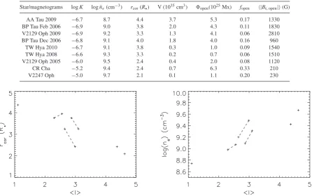
in-creasing distance from the star is the dominant factor. In Fig.6,
we show that there is an anticorrelation between the closed coronal extent and the field complexity for the stars in the sample. Simpler fields are able to hold on to the hot coronal plasma much further from the stellar surface than more complex fields. AA Tau, which has the simplest field in the sample, has a closed corona that extends
out to 4.5R. V2247 Oph, which has a much more complex field,
has a closed corona that only extends out to 2R.
The other factors that determine the closed coronal extent are the stellar mass, the coronal temperature and the rotation rate (Jardine
& Unruh1999; Jardine et al.2006). Decreasing the stellar mass
leads to a larger surface gravity and a smaller pressure scaleheight; increasing the coronal temperature or the rotation rate leads to an
increased pressure scaleheight.3Due to the slow rotation rates of
the CTTSs considered here, centrifugal stripping does not have a
3Increasing the stellar rotation rate also moves the corotation radius inwards. This can be significant for the closed coronal extents for rapidly rotating stars because inside of the corotation radius, the thermal pressure inside of a closed coronal loop decreases with increasing distance from the star, whereas outside of the corotation radius, the thermal pressure increases with increasing distance from the star (Jardine & Unruh1999). This effect is not taken into account here because we assume in our coronal models that the source surface is at the corotation radius, and therefore no closed coronal loops can extend past this radius.
at Library & Information Services, University of St Andrews on January 13, 2014
http://mnras.oxfordjournals.org/
Table 3. Results from the coronal plasma model for each of the stars in the sample. The maps are arranged from top to bottom by descending strength of the dipole component of the field. From left to right, the columns correspond to the proportionality parameterKbetween the magnetic pressure and the plasma pressure at the base of the corona fitted to the observed coronal emission measures, the emission measure weighted average coronal electron density, the maximum radius at which the stellar magnetic field can contain the hot coronal plasma, the volume of the closed corona, the open unsigned magnetic flux, the fraction of the stellar surface covered in open field and the average field strength in regions of the stellar surface covered in open field.
Star/magnetograms logK log ¯ne(cm−3) rcor(R) V (1035cm3) open(1025Mx) f
open |Br, open|(G)
AA Tau 2009 −6.7 8.7 4.4 3.7 5.3 0.17 1330
BP Tau Feb 2006 −6.9 9.0 3.8 2.0 4.3 0.11 1830
V2129 Oph 2009 −6.9 9.2 3.3 1.3 4.1 0.06 2810
BP Tau Dec 2006 −6.8 9.1 4.0 1.8 4.0 0.16 960
TW Hya 2010 −6.7 9.1 3.8 0.3 1.0 0.09 1540
TW Hya 2008 −6.6 9.3 3.3 0.2 0.7 0.06 1510
V2129 Oph 2005 −6.0 9.5 2.4 0.4 2.0 0.08 1120
CR Cha −5.2 9.4 2.4 0.7 6.3 0.33 210
V2247 Oph −5.0 9.7 2.1 0.1 1.1 0.20 230
Figure 6. Results of the coronal X-ray emitting plasma model. Left-hand panel: the maximum radius to which the stellar magnetic fields can contain the hot coronal plasma as a function ofl. Right-hand panel: the emission measure weighted average coronal electron density as a function ofl. These figures show that simple magnetic fields lead to extended, diffuse coronae and complex fields lead to compact, dense coronae. Data points representing the same star from two different epochs are connected by dashed lines.
significant effect on the sizes of the closed coronae of these stars. The lack of clear correlations between coronal temperature and closed coronal extent, and between stellar mass and closed coronal extent indicates that coronal temperature and stellar mass are not as important in determining the closed coronal extent as magnetic field complexity.
For each of the stars, we calculate the emission measure weighted average coronal electron density for the modelled coronae and find
values of ¯ne between 108.7 and 109.9 cm−3. As shown in Fig. 6,
the stars with more complex fields, and more compact coronae, have much higher average electron densities. There is an order of magnitude variation between the minimum and the maximum electron densities in the sample. This is similar to the result of
Jardine et al. (2006) who found that stars with simple field structures
tend to have average coronal electron densities that are an order of magnitude lower than stars with more complex fields. The absence of magnetic flux on small scales in the ZDI magnetic maps can lead to an underestimation of the modelled electron densities (Johnstone
et al.2010).
For each of the stars, our calculations of the open unsigned mag-netic flux is based on both the PFSS model and the plasma model. We assume that a field line is open if it extends from the stellar
sur-face to the source sursur-face, or if the plasma-βis greater than unity
at any point along its length. The open unsigned magnetic flux can
be written as a function of two parameters: these are the average radial field strength at the stellar surface in regions of open field,
|Br,open|and the area of the stellar surface covered in open field,
4πR2
fopen, wherefopenis the open flux filling factor. The open flux
filling factor can have an effect on the properties of stellar winds launched from coronal holes. By analogy with the solar wind, larger
values offopenlead to smaller coronal expansion factors (i.e. smaller
rates of expansion of magnetic flux tubes with increasing distance from the star) which can lead to stellar winds that are slower and
more dense (Wang & Sheeley1990; Arge & Pizzo2000; McGregor
et al.2008). The open magnetic flux is given by
open=4πR2fopen|Br,open|. (15)
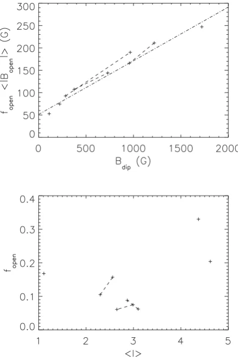
The values offopenand|Br,open|are given in Table3. In Fig.7, we
show that the value offopen|Br,open|is determined by the strength
of the dipole component of the field. This means that for each star, the open unsigned magnetic flux is determined by the strength of the dipole component and the surface area of the star. The following relation is derived from the linear fit to the results presented in
Fig.7:
openR−2=1.5Bdip+644.0 G. (16)
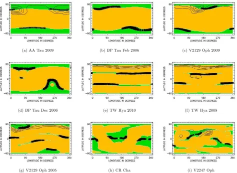
The locations of open and closed field structures for each of the
stars in the sample are shown in Fig.8. The distributions of these
at Library & Information Services, University of St Andrews on January 13, 2014
http://mnras.oxfordjournals.org/
Figure 7. Upper panel: correlation between the strength of the dipole com-ponent andfopen|Br,open|, wherefopenis the fraction of the stellar surface covered in open flux and|Br,open|is the average radial field strength in re-gions of open flux over the stellar surface. By definition,fopen|Br,open| = open/4πR2, whereopen is the unsigned open magnetic flux. The data is well fitted by the relationfopen|Br,open| =0.12Bdip+51.3 G. Lower panel: correlation between the fraction of the stellar surface covered in regions of open flux,fopen, and the parameterl, which is related to the complexity of the magnetic field and the rate at which the field strength falls off with increasing distance from the star. Data points representing the same star from two different epochs are connected by dashed lines.
structures are a strong function of field complexity, with regions of open flux covering the magnetic poles on all stars. Simple axisym-metric dipole fields such as the one seen on AA Tau have regions of open flux predominantly at high latitudes, with all low-latitude field structures being closed, and regions of open flux covering 10–20 per cent of the stellar surface. More complex fields, such as that seen on V2247 Oph, show open flux distributed over all
latitudes, covering≈20 per cent of the stellar surface. Fields that
are dominated by large-scale octupole components, such as those seen on TW Hya and V2129 Oph, tend to have regions of open flux at mid-latitudes extending in bands around the star, with only 5–10 per cent of the stellar surface covered in regions of open field. The range of values of the open flux filling factors found here are in good agreement with those found for the Sun by applying the PFSS model to the observed surface magnetic field maps (Wang & Sheeley 1990).
5 D I S C T R U N C AT I O N A N D AC C R E T I O N
5.1 Model
In this section, we use a simple model to investigate disc truncation and magnetospheric accretion geometries. We assume that the disc is truncated by the stellar magnetic field and accretion occurs along all field lines that connect to the disc between the disc truncation radius and the outer radius at which that magnetic field can begin to deflect material out of the disc plane and into an accretion column. We therefore need to estimate the disc truncation radius and the outer radius at which the magnetic field is able to disrupt the disc for each star in the sample.
We assume that the disc truncation radius is at the Alfv´en radius where the magnetic energy density is balanced by the kinetic energy
density from the disc: this is whereρ(r)v(r)2/2=B(r)2/8π, where
ρ is the mass density of material in the disc,vis the velocity of
material in the disc (approximately equal to the Keplerian orbital
velocity in this case) andBis the stellar magnetic field strength.
Making this assumption, Elsner & Lamb (1977) derived an
expres-sion for the case of isotropic spherical accretion of material falling at free-fall speeds on to a star. Conservation of mass and the isotropic density distribution mean that the mass accretion rate is given by
˙
Ma=4πr2ρ(r)v(r) and the free-fall assumption means that the
in-fall velocity of accreting material is given byv(r)=(GM/r)1/2.
This implies that the Alfv´en surface is where
B2=C
(GM)1/2Mar˙ A−5/2 (17)
whererAis the Alfv´en radius andCis a factor [not present in the
Elsner & Lamb (1977) formulation] that accounts for the
differ-ence between magnetospheric accretion from a disc and spherical
accretion. Elsner & Lamb (1977) assumed that the star’s magnetic
field is a simple dipole, such thatB= μ1r−3, whereμ1=BR3
andBis the stellar surface magnetic field strength (in the case of
accretion from a disc with a axisymmetric dipole field, this can be taken as the field strength in the equatorial plane). Substituting this into equation (17) gives the familiar expression
rA=2−1/7k
B2 R6
(GM)1/2Ma˙
2/7
, (18)
wherekis another factor that accounts for the difference between
magnetospheric accretion from a disc and spherical accretion and
is given byk=(2−1/2C)−2/7. Long, Romanova & Lovelace (2005)
used MHD accretion simulations to estimatek∼0.5 for
magneto-spheric accretion from a disc. We assumeC∼16 in equation (17),
because this is equivalent tok∼0.5 in equation (18). For each of
the stars, we solve equation (17) using field extrapolations without
a source surface and by takingB2at each radius as the longitudinal
average value ofB2in the equatorial plane.
An outer estimate for the radius at which the magnetic field can affect accretion is the radius at which the magnetic torque on the disc is balanced by the internal viscous torque (e.g. Bessolaz et al.
2008); we call this the torque balance radiusrt. Due to the difference
in rotation rate between the disc and the stellar surface (except for at the corotation radius), the magnetic field lines connecting the star and the disc become twisted. As in previous studies (e.g. Clarke et al.
1995; Wang1996; Gregory et al.2008) we assume that this twist is
45◦, and so|Bz| = |Bφ+|, whereBφ+is the longitudinal component of
the magnetic field that is generated by the twisting of magnetic field
at Library & Information Services, University of St Andrews on January 13, 2014
http://mnras.oxfordjournals.org/
Figure 8. Surface maps showing the predicted locations of open magnetic field (green), closed magnetic field (yellow) and accretion footpoints (black) for most of the stars in the sample. The black contour lines show the locations of excess CaIIIRT emission inferred from Doppler imaging; this is considered a good observational constraint on the locations of accretion footpoints. These maps are arranged from left to right and from top to bottom by decreasing strength of the dipole components of the field.
lines by the inner edge of the circumstellar disc. In the equatorial
planeBz=Bθ, so the torque balance radius can be found by solving
B2 θrt2=
1
2Ma˙
GM rt
1/2
, (19)
where we findrtusing field extrapolations without a source surface
and taking B2
θ at each radius as the value of Bθ2 averaged over
all longitudes in the equatorial plane. As in Clarke et al. (1995),
if we assume that the field is an axisymmetric dipole, such that Bθ=BR3
r−3, the torque balance radius is given by
rt=22/7
B2 R6
(GM)1/2Ma˙
2/7
. (20)
Since accretion cannot occur on to the star from regions of the
disc outside of the corotation radius, in cases where we calculatert
to be outside the corotation radius, we take the outer radius at which accretion can occur to be the corotation radius.
In several cases, the torque balance radii and the Alfv´en radii will
be overestimated because the quantity ˙Maused in the two above
equations is a measure of the rate at which mass moves inwards through the disc (introduced into the equations because the viscosity in the disc is not well understood), and not a measure of the rate at which material accretes on to the central star. Since some disc material will be lost in the form of disc winds, and not accrete on
to the central star, the measured mass accretion rates underestimate the rate at which mass moves inwards through the disc.
For comparison, we also calculate the disc truncation radii using
the alternative formulation of Bessolaz et al. (2008), given by
rtrunc=2m2s/7
B 140
4/7 Ma˙
10−8
−2/7 M
0.8
−1/7R
2
5/7 ,
(21)
wherems∼1, and the quantitiesB, ˙Ma,M andRare in units
of G, Myr−1, M
and R, respectively. The results from these
calculations can be seen and compared with therAandrtestimates
in Table4and Fig.12.
In order to estimaterA,rtandrtruncfor each star, we adopt the same
mass accretion rates as used in the papers where the magnetic maps
were presented, as listed in Table1. These values were calculated
from the same observations that were used to derive the magnetic maps and are therefore the most appropriate for these calculations. When the inner and outer radii from which accretion can occur are estimated, we use PFSS extrapolations with the source-surface radius set to the corotation radius, and trace field lines from ev-ery point in the disc from which accretion can occur and assume that all such field lines support accretion. We assume that accre-tion only occurs along the field line in the direcaccre-tion at which the component of effective gravity along the field line in a coordinate
at Library & Information Services, University of St Andrews on January 13, 2014
http://mnras.oxfordjournals.org/
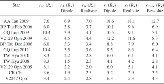
Table 4. Results of the disc truncation radius calculations. The maps are arranged from top to bottom by descending strength of the dipole component of the field. From left to right, the columns correspond to the Alfv´en surface radius calculated assuming the field is an axisymmetric dipole (equation 18), the Alfv´en radius calculated using potential field extrapolations of the ZDI magnetic maps (equation 17), the torque balance radius calculated assuming the field is an axisymmetric dipole (equation 20), the torque balance radius calculated using potential field extrapolations of the ZDI magnetic maps (equation 19) and the alternative formula (equation 21) of Bessolaz et al. (2008).
Star rco(R) rA(R) rA(R) rt(R) rt(R) rtrunc(R) Dipole Realistic Dipole Realistic Bessolaz
AA Tau 2009 7.6 6.9 7.0 18.6 18.1 12.7
BP Tau Feb 2006 6.0 3.8 3.7 10.1 9.6 6.9
GQ Lup 2009 10.4 3.9 4.1 10.5 9.1 7.1
V2129 Oph 2009 8.1 4.5 4.4 12.2 11.6 8.3
BP Tau Dec 2006 6.0 3.3 3.4 8.8 7.9 6.0
GQ Lup 2011 10.4 3.5 3.6 9.5 8.3 6.4
TW Hya 2010 8.3 2.2 2.8 6.0 6.1 4.1
TW Hya 2008 8.3 1.5 2.3 4.1 4.2 2.8
V2129 Oph 2005 8.1 2.2 2.0 6.0 5.1 4.1
CR Cha 3.6 1.9 2.5 5.2 2.9 3.5
V2247 Oph 3.4 2.4 2.8 6.3 5.3 4.3
system corotating with the star points inwards towards the stellar surface.
Johnstone et al. (2010) showed that the possible absence of
mag-netic flux on small scales in the ZDI magmag-netic maps is unlikely to have a significant effect on accretion models. This is because accretion is affected primarily by the large-scale structure of the stellar magnetic field, with the small-scale structures having little significance.
5.2 Results
In Table4, we give the values of the Alfv´en surface radii and the
torque balance radii for each of the stars. These have both been calculated twice: first by assuming that the field is an axisymmetric dipole with the polar field strength of the dipole taken to be that of the dipole component derived from the ZDI magnetic maps, and then using the potential-field extrapolations of the ZDI magnetic
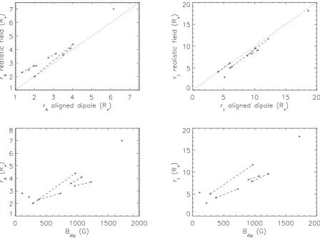
maps. In Fig.9, we show the relation between the results calculated
using the two methods (i.e. using the assumption of an axisymmetric dipole field, and using the potential field extrapolations from the ZDI maps) for both the Alfv´en surface radii and the torque balance radii. In general, the values are similar, indicating that it is reasonable to approximate the field as an axisymmetric dipole when calculating the disc truncation radius using the analytic formulations described above, though it is necessary to consider higher order spherical harmonic components when describing the flow of matter on to the
stellar surface (Gregory & Donati2011; Adams & Gregory2012).
However, the disc truncation radius can only be estimated if the strength of the dipole component of the field is accurately known. In many cases, what is actually known is the surface averaged field strength that takes into account every component of the field, and
not just the dipole. In Fig.10, we show that there is only a weak
correlation between the surface averaged magnetic field strength derived from the ZDI map and the strength of the dipole component of the field. This figure does not take into account the fact that most of the magnetic flux on small scales that could be measured by Zeeman broadening techniques is not captured in the ZDI maps. It is not possible to accurately estimate the strength of the dipole component of a field, and therefore the disc truncation radius, if the only quantity known is the surface averaged field strength.
The differences between the Alfv´en surface radii calculated us-ing the two methods is a result of two factors: the tilt of the dipole component of the field relative to the rotation axis and the pres-ence of the octupole component. The tilt in the dipole component increases the field strength in the equatorial plane relative to what it would be for an axisymmetric dipole. This pushes the inner edge of the disc away from the star. This is significant for the CR Cha field and the TW Hya 2008 field because they have significantly tilted dipole components. The effect of the octupole component of the field depends on whether it is aligned or anti-aligned with the dipole component (i.e. whether the positive magnetic pole of the octupole component is in the same hemisphere as the positive magnetic pole or the negative magnetic pole of the dipole com-ponent). If the octupole component is aligned with the dipole, the two components will add up destructively in the equatorial plane, leading to a weaker field and a smaller Alfv´en surface radius. If the octupole component is anti-aligned with the dipole, the two com-ponents add up constructively in the equatorial plane, leading to a stronger field and a larger Alfv´en surface radius. The effects of parallel and antiparallel dipole and octupole components are
dis-cussed in detail in Gregory & Donati (2011) and Adams & Gregory
(2012).
In general, the discs are truncated several stellar radii from their stars, with AA Tau having the largest truncation radius. This is unsurprising given AA Tau’s strong dipolar magnetic field. The truncation radius for AA Tau is close to the corotation radius, which
is consistent with the observations of Bouvier et al. (1999) and
Bouvier et al. (2003) that showed that the star is being eclipsed
periodically by a warped inner edge of its disc, with the warp located at approximately the corotation radius.
We show in Fig.9that stars with weaker dipole components
tend to have smaller Alfv´en surface radii; however, the stellar mass, stellar radius and mass accretion rate are also very important in determining the Alfv´en surface radius. For CV Cha, which has a weak dipole component and a large measured mass accretion rate, the magnetic field is not able to truncate the disc outside of the star, and so we do not consider it here.
The torque balance radii are generally significantly larger than the Alfv´en surface radii. The exception to this is CR Cha, where the large tilt in the dipole component means that the method used for
at Library & Information Services, University of St Andrews on January 13, 2014
http://mnras.oxfordjournals.org/
Figure 9. Upper-left panel: Alfv´en surface radii calculated from realistic field structures using equation (17) against the values calculated by assuming that the fields are axisymmetric dipoles using equation (18). Lower-left panel: Alfv´en surface radii calculated from realistic field structures against the strengths of the dipole components of the fields. Upper-right panel: torque balance radii calculated from realistic field structures using equation (19) against the values calculated by assuming that the fields are axisymmetric dipoles using equation (20). Lower-right panel: torque balance radii calculated from realistic field structures against the strengths of the dipole components of the fields. Data points representing the same star from two different epochs are connected by dashed lines. CV Cha, V4046 Sgr A and V4046 Sgr B are not included.
Figure 10. Dipole field strength against surface averaged field strength for the sample of CTTS ZDI maps. The solid line shows the line of equality, and the dotted lines show the lines ofBdip=2BandBdip= B/2. The two stars in the binary system V4046 Sgr are shown as open circles. Data points representing the same star from two different epochs are connected by dashed lines. The surface averaged field strengths should be considered as lower limits because they do not take into account missing magnetic flux on small scales. This figure shows that the surface averaged magnetic field strengths are not reliable indicators of the dipole field strength.
calculating the torque balance radii is not valid because the method assumes that the magnetic field lines threading the disc are vertical prior to being disturbed by the orbital motion of the disc mate-rial, which is not the case for a significantly tilted dipole. For AA Tau especially, due to its strong axisymmetric dipole component, the torque balance radius is very large, indicating that AA Tau’s magnetic field may be able to disrupt the disc well outside the coro-tation radius. For V2129 Oph, the 2005 field has a torque balance radius inside the corotation radius, but due to the large increase in the strength of the dipole component, the 2009 field has a torque balance radius that has moved outside of the corotation radius.
In Fig.8, we show the locations of the predicted accretion
foot-points for each of the stars in the sample. These locations are highly dependent on magnetic field structure.
For the most dipolar fields, such as the AA Tau field, the two BP Tau fields, and the V2129 Oph 2009 field, the accretion foot-points are all at high latitudes. These are also the fields with the
lowest values ofl. The simple fields also have the strongest dipole
components, and therefore have the largest disc truncation radii. As these fields have strong dipole components, and the discs are truncated far from the stellar surfaces, the fields are very dipolar at the inner disc edges, and accretion happens along large-scale field lines that connect with the stellar surface at high latitudes. The field
structure and accreting field lines for AA Tau are shown in Fig.11.
at Library & Information Services, University of St Andrews on January 13, 2014
http://mnras.oxfordjournals.org/
[image:13.595.43.283.471.632.2]