Testing the validity of the ‘local’ and ‘global’ GKLS master equations on an exactly solvable model

J. Onam Gonz´alez,1, 2,∗Luis A. Correa,2,†Giorgio Nocerino,2,‡Jos´e P. Palao,1,§Daniel Alonso,1,¶and Gerardo Adesso2,∗∗ 1_{Dpto. de F´ısica and IUdEA: Instituto Universitario de Estudios Avanzados, Universidad de La Laguna, 38203 Spain}

2_{School of Mathematical Sciences and Centre for the Mathematics and Theoretical Physics of Quantum Non-Equilibrium Systems,}

The University of Nottingham, University Park, Nottingham NG7 2RD, United Kingdom

(Dated: September 26, 2017)

When deriving a master equation for a multipartite weakly-interacting open quantum systems, dissipation is often addressed locallyon each component, i.e. ignoring the coherent couplings, which are later added ‘by hand’. Although simple, the resulting local master equation (LME) is known to be thermodynamically inconsistent. Otherwise, one may always obtain a consistentglobalmaster equation (GME) by working on the energy basis of the full interacting Hamiltonian. Here, we consider a two-node ‘quantum wire’ connected to two heat baths. The stationary solution of the LME and GME are obtained and benchmarked against the exact result. Importantly, in our model, the validity of the GME is constrained by the underlying secular approximation. Whenever this breaks down (for resonant weakly-coupled nodes), we observe that the LME, in spite of being thermodynamically flawed: (a) predicts the correct steady state, (b) yields the exact asymptotic heat currents, and (c) reliably reflects the correlations between the nodes. In contrast, the GME fails at all three tasks. Nonetheless, as the inter-node coupling grows, the LME breaks down whilst the GME becomes correct. Hence, the global and local approach may be viewed ascomplementarytools, best suited to different parameter regimes.

PACS numbers: 05.70.-a, 05.30.-d, 03.65.Yz

I. INTRODUCTION

The Gorini-Kossakowski-Lindblad-Sudarshan (GKLS) quantum master equation [1,2] is central in the theory of open quan-tum systems. It reads

dρρρ

dt =Lρρρ=− i ¯

h[HHH,ρρρ] +Dρρρ=− i ¯

h[HHH,ρρρ] +

∑

A

AA_kρρρAAA†_k−1 2AAA

† kAAAkρρρ−

1 2ρρρAAA

† kAAAk

, (1)

and generates a quantumdynamical semigroup, i.e. it gives rise to a dynamical map ρρρ(t) =V(t)ρρρ(t0) =eL(t−t0)ρρρ(t0) with the semi-group propertyV(t)V(s) =V(t+s). This type of memoryless or Markovian evolution arises naturally when an open quantum system couples weakly to an environment at inverse-temperatureβ= (kBT)−1, so that the typical relaxation time is by far the largest scale in the problem [3].

Among many others, Eq. (1) has the following key properties:

(i) It ensures acompletely positivedynamics which, in turn, implies that the relative entropyS(ρρρ1|ρρρ2):=tr{ρρρ1(logρρρ1−logρρρ2)} between any two states evolving underV(t)decreasesmonotonically, i.e. _dtdS(ρρρ1(t)|ρρρ2(t))≤0 [4,5].

(ii) Under mild assumptions, the thermal stateτττ∝exp(−βHHH)is theonly stationary stateofV(t), i.e. Lτττ=0 [6]. That is, Eq. (1) describes relaxation towards thermal equilibrium.

Interestingly, one may use Eq. (1) to model a continuous (quantum) thermodynamic cycle [7,8]. By coupling the open system (i.e. theworking substance) to various heat baths at different temperatures and possibly also to a periodic external drive, a stationary non-equilibrium state builds up. The direction of the corresponding steady-state heat currents may be controlled by suitably engineering the spectrum of the working substance. Hence, we can speak of ‘quantum heat engines’ or ‘quantum compression/absorption refrigerators’ [9], which have attracted a lot of attention in recent years [10–14].

In such quantum heat devices, the stationary incoming heat currents{Q˙α}and the power output−Pare defined as [7]

d

dttr{HHHρρρ∞}=0=P+

∑

∂HHH

∂t ρρρ∞

+

_∑

tr{HHHDαρρρ∞}, (2)

∗_{[email protected]}

†_{[email protected]} ‡_{[email protected]} §_{[email protected]}

¶_{[email protected]}

∗∗_{[email protected]}

whereρρρ∞is the steady state of the working substance, andDα denotes the GKLS dissipation super-operator associated with bathα.

Owing to properties (i) and (ii) above, the stationary heat currents ˙Qα satisfy the relation ∑αQ˙α/Tα ≤0, which is the Clausius inequality. In other words, addressing the dynamics of quantum heat devices with GKLS quantum master equations ensures thermodynamic consistency.

When modelling open quantum systems made up of multiple weakly-interacting parts coupled to local environments, it is commonplace to build the corresponding master equation by simply adding the local dissipators for the relaxation of each individual component (ignoring their coherent interactions). That is, for a multipartite system with HamiltonianHHH=∑jhhhj+kVVV, whereVVV contains all the internal couplings (of strengthk), one would write1

dρρρ dt =−

i ¯

h[HHH,ρρρ] +

∑

(k=0)

α ρρρ. (3)

Although Eq. (3) is in GKLS form, property (ii) ceases to hold, as the dissipatorsD(k=0)α do not match the HamiltonianHHH, but rather the non-interacting∑jhhhj. Consequently, describing heat transport with the local master equation (3) may lead to thermodynamic inconsistencies: Heat could, for instance, flow against the temperature gradient [15], or non-vanishing steady-state heat currents could be present even if all reservoirs are set to the same temperature [16].

These observations, strongly advise to follow the standard procedure to consistently obtain the correct global dissipatorsDα [3]. However, doing so may become particularly challenging when dealing with large systems, e.g. long harmonic or spin chains. Moreover, in such cases the capital assumption that the dissipation time scale is by far the largest in the problem is likely to break down as the spectrum of the system becomes denser [17]; Eq. (1) would then lack a microscopic justification. These difficulties explain the popularity of simple approaches based on weak internal coupling approximations such as Eq. (3) [17,18]. In this paper we wish to put such local approaches to the test.

In particular, we choose an exactly solvable model consisting of a two-node harmonic chain weakly coupled on both edges to two heat baths at different temperatures. Our system is set up so that, when the inter-node coupling strength becomes comparable or smaller than the node-baths dissipative couplings, the secular approximation underlying Eq. (1) may break down. This allows us to gauge to which extent the local master equation (LME) remains an accurate description. Interestingly, we find that the local approach yields an excellent approximation to the steady state, the stationary heat currents, and the asymptotic quantum and classical correlations, in the regime of parameters in which the global master equation (GME) fails even qualitatively. More generally, it follows that heat conduction through arbitrarily large harmonic chains can be correctly modelled within the local approach always provided that the internal couplings are sufficiently weak. The present work thus adds to the efforts of Refs. [15–24] to clarify thedos and don’tsof modelling heat transport through multipartite open quantum systems.

This paper is structured as follows: In Sec.II Awe outline the steps of the microscopic derivation of the GKLS quantum master equation. We then proceed to derive and solve such an equation for our specific model in SecII B. The alternative local master equation is obtained in Sec.II C. Before proceeding to benchmark both approaches, in Sec.IIIwe sketch how the exact steady-state solution of the system may be obtained by solving the quantum Langevin equations. We then devote Sec.IVto present and discuss our results. Finally, in Sec.Vwe summarize and draw our conclusions.

II. DERIVING MARKOVIAN MASTER EQUATIONS A. The model, the Markovian master equation and its steady state

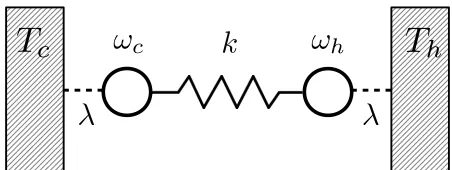
We will consider a two-node ‘quantum wire’ (see Fig.1) consisting of mechanically-coupled harmonic oscillators with bare frequenciesωc andωhand coupling strength k>0. Each node will be weakly connected to a bosonic bath, i.e. an infinite collection of uncoupled harmonic modes in thermal equilibrium (at temperaturesTc<Th). The total Hamiltonian may be cast as

H

HH=

_∑

α∈{c,h}

ω_α2 2 XXX

2 α+

P P P2_α

2 !

+k

2(XXXc−XXXh) 2₊

∑

α∈{c,h}

∑

ω_α2_,µmα,µ

2 xxx 2 α,µ+

p p p2_α,µ

2mα,µ !

−

_∑

α∈{c,h}

X XXα⊗

∑

µ

gα,µxxxα,µ, (4)

where the masses of the nodes have been set tomc=mh=1, and the constantsgα,µ stand for the coupling strength between nodeα and each of the environmental modes(α,µ). Also, in all what follows we shall set ¯hand the Boltzmann constantkBto 1. We will refer to the first three terms in the right-hand side of Eq. (4) as the free (system + baths) HamiltonianHHH0=HHHS+HHHB,

FIG. 1. Schematic representation of the wire. The two harmonic nodes at frequenciesωcandωhare coupled through a spring-like interaction of strengthk. Each node is, in turn, dissipatively coupled to a ‘cold’ and ‘hot’ heat bath at temperaturesTc<Th. The dissipation strengthλ2is assumed sufficiently weak to jus-tify the use of a perturbative master equation up toO(λ2).

as opposed to the last termHHHint, which describes the system-baths interaction. For later convenience, we shall also introduce the notationBBBα:=∑µgα,µxxxα,µ.

We will group the system-baths cupling constants in thespectral densityfunctions defined asJα(ω):=π∑µ g2_α,µ

2mµωµδ(ω−ωµ).

In particular, we will choose 1D baths with the Ohmic form

Jc(ω) =Jh(ω) =λ2ω Λ2

ω2+Λ2, (5)

whereΛis a high-frequency cutoff(max{ωc,ωh} Λ)and the parameterλ captures thedissipation strength. Note that the bath operatorsBBBαare thusO(λ).

For completeness, we will now briefly sketch a simple procedure to obtain the standard second-order Markovian generator for the reduced dynamics of the system (see Ref. [3] for full details). Let us take the Liouville-von Neumann equation in the interaction picture

d ˜ρρρ(t) dt =−i[

˜ H H

Hint(t),ρρρ˜(t)], (6)

where ˜HHHint(t):=eiHHH0tHHHinte−iHHH0tt and[·,·]stands for a commutator. Formally integrating Eq. (6) and assuming that the initial condition is such that tr{ρρρ˜(0)HHH˜int}=0 yields the following equation of motion for the system:

d ˜σσσ dt =−

Z t

0

dstrB[HHH˜int(t),[HHH˜int(s),ρρρ˜(s)]]. (7)

Here, ˜σσσ:=trBρρρ˜ and trB{· · · }denotes trace over the baths. We will now assume that the dissipation strengthλ is so weak that when starting from a factorized initial conditionρρρ0:=σσσ(0)⊗τττc⊗τττhthe propagated state ˜ρρρ(t)'σσσ˜(t)⊗τττc⊗τττhremains approximately factorized at all times.τττα∈{c,h}are thermal states for the hot and cold bath. We will also replace ˜σσσ(s)inside the integral in Eq. (7) by ˜σσσ(t), thus making it time-local. The change of variabless→t−syields the Redfield equation [25,26]

d ˜σσσ dt ' −

Z t

0

dstrB[HHH˜int(t),[HHH˜int(t−s),σσσ˜(t)⊗τττc⊗τττh]]. (8)

Notice that the resulting stateρρρ(t) does keep a memory of the initial conditionρρρ(0)and hence, Eq. (8) is non-Markovian. However, provided that the integrand above decays sufficiently fast, one might sett→∞in the upper limit of integration, which is referred-to as Born-Markov approximation. This approximation is justified wheneverλ2min{T,Λ}.

A further step still remains to be undertaken in order to bring the resulting ‘Markovian Redfield’ master equation to the canon-ical GKLS form—the secular approximation. Let us examine ˜HHHint(t)more closely. One may always decomposeXXXα=∑ωLLL

ω α, where[HHHS,LLLωα] =−ωLLL

ω

α, so that ˜HHHint=∑ωe −iωt_LLLω

α⊗BBB˜α(t), with the interaction-picture bath operator ˜BBBα(t) =eiHHHBtBBBαe−iHHHBt. Plugging this into Eq. (8) leads to

d ˜σσσ dt '

1 2

∑

∑

ω,ω0

ei(ω0−ω)t γα(ω)

L LLω

ασσσ˜LLL ω0 α

† −LLLω0

α †

L LLω

ασσσ˜

+h.c., (9)

whereγα(ω) =2Re R∞

0 ds eiωstrB{BBBα(t)BBBα(t−s)}. Note that we are completely ignoring Im R∞

0 ds eiωstrB{BBBα(t)BBBα(t−s)}, which would eventually lead to a mere shift (of orderλ2) on the energy levels of the Hamiltonian (Lamb shift) [3]. The secular approximation consists in time-averaging Eq. (9) over an interval of the order of the dissipation timeTD∼λ−2. All terms with ω06=ωabove can then be discarded provided that they oscillate fast as compared withTD. Returning to the Schr¨odinger picture, finally leaves us with the GKLS quantum master equation

dσσσ

dt ' −i[HHHS,σσσ] +

∑

∑

∑

L LLω

ασσσLLL ω α †

−1

2{LLL ω α †

LLLω α,σσσ}+

where{·,·}+stands for anti-commutator. In the next section, we will concentrate in obtaining the specific form of the operators

LLLω

α for the Hamiltonian in Eq. (4).

Because Eq. (4) is overall quadratic in position and momenta, the steady state will be Gaussian and thus, fully characterized by its first and second order moments [27]. In fact, one can easily see thathXXXαi=hPPPαi=0, whereh·idenotes stationary average. As a result, the steady state will be specified only by the 4×4covariance matrix, with elements[Γ]_kl :=₂1h{RRRk,RRRl}+i, with

~_{RRR= (XXXc,PPPc,XXX}

h,PPPh)T.

Since we wish to calculate the covariances[Γ]_kl rather than the stateσσσ, it will be more convenient to work with theadjoint master equation [3] which, for an arbitrary system observable in the Heisenberg pictureOOO(t), reads

dOOO

dt 'i[HHHS,OOO] +

∑

†

αOOO=i[HHHS,OOO] +

∑

∑

ω γα(ω)

L L Lω

α †

O OOLLLω

α− 1 2{LLL

ω α †

L LLω

α,OOO}+

. (11)

B. The global master equation

The first step to derive consistentLLLω

α operators will be to rotateHHHSinto its normal modes. These are η

ηη+=cosϑXXXc−sinϑXXXh (12a)

η

ηη−=sinϑXXXc+cosϑXXXh, (12b)

where the angleϑ is

cos2ϑ =−δ 2 ω+

p

4k2_+δ4 ω 2p4k2_+δ4

ω

(13)

and, in turn,δ_ω2:=ω_h2−ω_c2. The corresponding normal-mode frequencies write as

Ω±2=

1 2

ω_c2+ω_h2+2k±q4k2_+δ4 ω

. (14)

After this transformation, the Hamiltonian (4) rewrites as

H H

H=

_∑

s∈{+,−}

Ω_s2 2 ηηη

2 s+

ΠΠΠ2_s 2

!

+HHHB−(cosϑ ηηη++sinϑ ηηη−)⊗BBBc+ (sinϑ ηηη+−cosϑ ηηη−)⊗BBBh, (15)

whereΠΠΠs=dηηηs/dt. By writingηηηs= (aaas+aaa†s)/ √

2Ωs(withaaas andaaa†s being annihilation and creation operators on modeΩs) one can see thatXXXα=LLL

Ω+ α +LLL

Ω−

α +h.c., whereLLL Ω+

c :=cosϑaaa+/ √

2Ω+,LLLΩc−:=sinϑaaa−/

√

2Ω−,LLLΩ_h+:=−sinϑaaa+/ √

2Ω+,

LLLΩ−

h :=cosϑaaa−/ √

2Ω−, andLLL−αΩ±:=LLL Ω± α

† .

Looking back to the right-hand side of Eq. (9), we see that there are 16 terms associated with 5 different open decay channels, oscillating asei(ω0−ω)t _{at frequencies|ω}0_{−ω|={0,2Ω}

+,2Ω−,Ω++Ω−,Ω+−Ω−}. Provided that the nodes are sufficiently

detuned, i.e.δωλ2, the secular approximation is guaranteed to be valid foranyvalue of the couplingk. However, ifωh−ωc became comparable or smaller than the dissipation strengthλ2, there would be no justification to discard the non-secular terms oscillating atΩ+−Ω−whenkbecomes very small. Indeed, definingR±:=2k±

p

4k2_+δ4

ωone may write

Ω+−Ω = s

ω_c2+ω_h2

2 

 s

1+ R+ ω_c2+ω_h2−

s

1+ R− ω_c2+ω_h2



 (16)

wheneverR±/(ω_c2+ω_h2)1, the Taylor expansion √

1+x=1+x₂−x2

8 +· · ·allows to approximate Eq. (16) as

Ω+−Ω−=

s

4k2_+δ4 ω 2(ω_h2+ω_c2)

+O R

2 + (ω_c2+ω_h2)3/2

!

. (17)

From Eq. (17) it is clear that for the secular approximation to be valid the dissipation rate must be such that

λ2 s

4k2_+δ4 ω 2(ω_h2+ωc2)

which, in the limit of resonant nodes simplifies toλ2k/ωc. Hence, we can anticipate that Eq. (10) will fail to describe nearly resonant weakly coupled nodes, which is precisely the regime in which we shall focus our analysis.

The only additional ingredient required to build Eq. (11) are thedecay ratesγα(±Ω±). A direct calculation leads to

γα(ω) =2J(ω)[1+nα(ω)], (19)

wherenα(ω):= (eω/Tα−1)−1 is the bosonic occupation number for frequencyω at temperatureTα. Note that γα(−ω) = exp(−ω/Tα)γα(ω). Combining all the above, and after tedious but straightforward algebra, we can obtain a closed set of equations of motion for the covariances2_hηηη2

±i,hΠΠΠ2±i, andh{ηηη±,ΠΠΠ±}+i. Note thath·idenotes here instantaneous average. d

dthηηη

2

±i=∆±hηηη2±i+h{ηηη±,ΠΠΠ±}+i+

Σ±

2Ω±

(20a)

d

dth{ηηη±,ΠΠΠ±}+i=2hΠΠΠ

2

±i −2Ω±hηηη2±i+∆±h{ηηη±,ΠΠΠ±}+i (20b) d

dthΠΠΠ

2

±i=∆±hΠΠΠ2±i −Ω±2h{ηηη±,ΠΠΠ±}+i+ Ω±

2 Σ±, (20c)

where the following notations have been introduced

∆+:= cos2ϑ

2Ω+

[γc(−Ω+)−γc(Ω+)] + sin2ϑ

2Ω+

[γh(−Ω+)−γh(Ω+)] (21a)

∆−:=

sin2ϑ 2Ω−

[γc(−Ω−)−γc(Ω−)] +

cos2ϑ 2Ω−

[γh(−Ω−)−γh(Ω−)] (21b)

Σ+:= cos2ϑ

2Ω+

[γc(−Ω+) +γc(Ω+)] + sin2ϑ

2Ω+

[γh(−Ω+) +γh(Ω+)] (21c)

Σ−:=

sin2ϑ 2Ω−

[γc(−Ω−) +γc(Ω−)] +

cos2ϑ 2Ω−

[γh(−Ω−) +γh(Ω−)]. (21d)

Below, it will be convenient to break down each of these coefficients into the sum of its two constituent terms, as∆±:=∆±c+∆±h

andΣ±:=Σ±c +Σ±h, where e.g.∆+c =cos2ϑ[γc(−Ω+)−γc(Ω+)]/(2Ω+). The further denotationsΣ±α=W−αΩ±+W α

Ω±, where e.g.Wc

−Ω+=cos 2

ϑ γc(−Ω+)/(2Ω+), will also be employed later on.

The stationary solution to Eq. (20) is simplyhηηη2±i=−Σ±/(2∆±Ω±),hΠΠΠ±i=−Ω±Σ±/(2∆±), andh{ηηη±,ΠΠΠ±}+i=0, so

that the non-zero elements of the asymptotic covariance matrix in the original quadratures reads

ΓG= 

   

[ΓG_]

11 0 [ΓG]13 0 0 [ΓG_]

22 0 [ΓG]24 [ΓG_]

13 0 [ΓG]33 0 0 [ΓG]24 0 [ΓG]44



   

, (22)

where[ΓG]11=hηηη2+icos2ϑ+hηηη2−isin2ϑ,[ΓG]22=hΠΠΠ2+icos2ϑ+hΠΠΠ2−isin2ϑ,[ΓG]33=hηηη2+isin2ϑ+hηηη2−icos2ϑ,[ΓG]44= hΠΠΠ2+isin2ϑ+hΠΠΠ2−icos2ϑ,[ΓG]13= (hηηη2−i − hηηη2+i)sinϑ cosϑ, and[ΓG]24= (hΠΠΠ2−i − hΠΠΠ2+i)sinϑcosϑ. Finally, the steady-state heat currents can be written as

˙ QG

α=tr{HHHSDασσσ(∞)}=hD†αHHHSi= 1

2

∑

s∈{+,−}

∆_sα

Ω_s2hηηη2_si+hΠΠΠ2_si

+ΩsΣsα

. (23)

Using Eqs. (21) we can cast (23) as

˙ QG

h =−Q˙Gc =

∑

Ωs

Wc ΩsW

h Ωs

Σs

(e−Ωs/Th_−e−Ωs/Tc_{), (24)}

from where it is clear thatTh>Tcentails ˙QGh =−Q˙Gc >0; that is, heatalwaysflows from the hotter bath into the colder one.

2_{It is indeed enough to consider the equations of motion for the mode occupation numbershaaa}†

C. The local master equation

Recall from Sec.Ithat, while thelocalmaster equation looks formally identical to the GME, the choice of operatorsLLLω α in the local approach is not consistent with the HamiltonianHHHS. As already advanced and provided that the couplingkis weak, one could derive two independent local dissipators D(k=0)α , acting on the cold and hot nodesseparately, to then construct an approximate equation of motion such as dσσσ/dt' −i[HHHS,σσσ] +∑α∈{c,h}Dα(k=0)σσσ, as an alternative to Eqs. (20). One might argue that this is a convenient strategy whenever finding all energy eigenstates of the full interacting Hamiltonian is hard, as these are required to write the decomposition{LLLω

α}of the system operator coupled to each bath [18]. In our simple example, however, the local approach leads to a more complicated dynamics than the global one—all 10 independent covariances are needed in order to obtain a closed set of equations of motion.

Specifically, within the local approach one decomposesXXXα=LLL ωα

α +LLL −ωα

α , whereLLL ωα

α :=bbbα/ √

2ωα,bbbα is an annihilation operator on nodeωα, andLLL

−ωα

α :=LLL ωα

α †

. The adjoint master equation Eq. (11) thus becomes

dOOO

dt 'i[HHHS,OOO] +

∑

α∈{c,h}

" γα(ωα)

2ωα

b b

b†_αOOObbbα− 1 2{bbb

†

αbbbα,OOO}+

+γα(−ωα) 2ωα

bbbαOOObbb

† α−

1 2{bbbαbbb

† α,OOO}+

#

. (25)

From (25), the equations of motion for the elements of the corresponding covariance matrixΓL_{are found to be}

d dthXXX

2

αi=h{XXXα,PPPα}+i+∆˜αhXXX2αi+ ˜ Σα 2ωα

(26a)

d dthPPP

2

αi=2khXXXα¯PPPαi −να2h{XXXα,PPPα}+i+∆˜αhPPP2αi+ ωαΣ˜σ

2 (α¯ 6=α) (26b)

d

dth{XXXα,PPPα}i=2hPPP

2

αi+∆˜αh{XXXαPPPα}+i −2να2hXXX 2

αi+2khXXXαXXXα¯i (α¯ 6=α) (26c) d

dthXXXαPPPα¯i=hPPPαPPPα¯i+khXXX

2 αi+

1

2(∆˜α+∆˜α¯)hXXXαPPPα¯i −ν 2 ¯

αhXXXαXXXα¯i (α¯ 6=α) (26d)

d

dthXXXcXXXhi=hXXXcPPPhi+hXXXhPPPci+ 1 2(

˜

∆c+∆˜h)hXXXcXXXhi (26e)

d

dthPPPcPPPhi= k

2 h{XXXh,PPPh}+i+h{XXXc,PPPc}+i

−ν_c2hXXXcPPPhi −νh2hXXXhPPPci+ 1 2(

˜

∆c+∆˜h)hPPPcPPPhi (26f)

whereνα2 :=ω 2

α+k, ˜∆α :=

γα(−ωα)−γα(ωα)

2ωα , and ˜Σα :=

γα(−ωα)+γα(ωα)

2ωα , and the angled brackets denote again instantaneous

average. The stationary solution of Eq. (26) is cumbersome but the steady-state heat currents can be compactly cast as

˙ QL

α= ˜ ∆α

2 h

ωα2hXXX 2 αi+hPPP

2

αi+k(hXXX 2

αi − hXXXαXXXα˜i) i

+Σ˜α 2

ωα+

k 2ωα

. (27)

As anticipated above and unlike Eq. (20), Eq. (26) does not necessarily yield a thermodynamically consistent steady state: One could even encounter striking situations for which ˙QL

h=−Q˙Lc <0 forTh>Tc or ˙QLα 6=0 forTh=Tc, as illustrated in [15,16].

D. Comment on the general validity of the local approach for modelling heat transport under weak internal coupling In spite of its thermodynamic inconsistencies, as it was pointed out in Ref. [18] the LME (25) can be formally understood as the lowest order in the perturbative expansionDα =D

(0) α +D

(1) α k+D

(2)

α k2+· · ·, whereD (0) α =D

(k=0)

α . The LME (25) would therefore be correct up toO(λ2k)and any thermodynamic inconsistency encountered should fall within this ‘error bar’.

Note that the GME is itself a perturbative master equation which neglects corrections of orderO(λ3)and below [28]. How-ever, it is guaranteed to give rise to thermodynamically consistent steady-state heat currents [7,10], as it enjoys the GKLS form (cf. Sec.I). Interestingly, it is the secular approximation which endows the GME with thermodynamic consistency: The Marko-vian Redfield equation (9), i.e. the previous step in the derivation of Eq. (10), is known to break positivity [28] and caution must be exercised when using it [29].

Coming back to our problem of describing heat transport in the limit of quasi-resonant weakly-coupled nodes, notice that the secular approximation is not problematic when invoked in the derivation of Eq. (25). Indeed, the operatorsLLLω

provided thatωαλ2and regardless of the detuning between the nodes. Consequently, and unlike Eq. (20), the LME should correctly describe the stationary properties of our system whenk/ωc.λ2.

More generally, one can claim that energy transport through an arbitrarily long harmonic chain is correctly captured by a LME within its range of validity; that is, whenever the inter-node couplings are weak. The claim can be made extensive to heat fluxes on spin chains, which were already addressed in Ref. [17] via a perturbative master equation relying on ‘weak internal couplings’, precisely in order to bypass the problems created in the GME by the secular approximation.

Finally, let us note that a natural alternative to the LME in our problem would be to incorporate the problematic decay channel of frequencyΩ+−Ω−into the GME, thus arriving to a partial Markovian Redfield equation (cf. Appendix). However, scaling

up the system in the number of nodes would quickly render this approach too involved to be practical.

III. EXACT NON-EQUILIBRIUM STEADY STATE

The steady state for an all-linear model can also be foundexactlyby solving the corresponding quantum Langevin equations [30–32]. In this section, we will limit ourselves to outline the procedure to calculate the stationary covariances for our particular problem, while full details on its application to similar settings can be found in e.g. Refs. [33–37].

To begin with, we must mention that the bare frequencies of the nodes need to be shifted so as to compensate for the distortion caused by the system-baths interaction. This eventually allows to recover the correct high temperature limit [31]. Hence, in the reminder of this section, we shall make the replacementωα27→ω˜

2

α, where ˜ω 2 α:=ω

2 α+∑µg

2

α,µ/(mα,µωα2,µ). For our choice of spectral density (5), the shift amounts simply toπ−1R₀∞dωJ(ω)/ω=λ2Λ.

Starting from Eq. (4), one may write the Heisenberg equations of motion for all degrees of freedom. Formally solving for xxxα,µ and inserting the result into the equations forXXXαyields the quantum Langevin equations

d2XXXα dt2 +ω˜

2

αXXXα+k(XXXα−XXXα¯)− Z ∞

t0

dsχα(t−s)XXXα(s) =FFFα(t) (α¯ 6=α). (28)

These are the equations of motion for two coupled harmonic oscillators, each of which is perturbed by the noiseFFFα(t)and relaxes according to the dissipation kernelχα(t). Specifically, these are defined as

F F Fα:=

∑

µ

gα,µ h

xxxα,µ(t0)cosω0(t−t0) +

pppα,µ(t0)

mα,µωα,µ

sinωα,µ(t−t0) i

(29a)

χα(t):=

∑

g2_α,µ

mα,µωα,µ

sinωα,µtΘ(t) = 2 πΘ(t)

Z ∞

0

dωJ(ω)sinωt. (29b)

The only assumption that we will make in order to find the exact steady state is, once again, that system and baths are initialized in the factorized initial conditionρρρ0=σσσ(t0)⊗τττc⊗τττh. We shall also taket0→ −∞. Let us first concentrate on the (stationary) covariance 1₂h{XXXα(t),XXXα0(t)}+i, which may be written in terms of the Fourier transform ˆXXXα(ω):=

R∞

−∞dt XXXα(t)e

iωt_as

1

2h{XXXα(t),XXXα0(t)}+i= 1 2

Z ∞

−∞ dω0

2π Z ∞

−∞ dω00

2π h{XXXˆα(ω

0_),XXXˆ α0(ω

00_)}

+ie−i(ω 0₊

ω00)t_{. (30)}

In turn, ˆXXX(ω)α can be directly found after Fourier-transforming Eqs. (28), which yields

ˆ X X Xc

ˆ XXXh

!

:=A−1 FFFˆ_ˆc F F Fh

! = ω˜

2

c−ω2+k−χˆc −k −k ω˜_h2−ω2+k−χˆh

!−1 ˆ F FFc

ˆ F F Fh

!

. (31)

From Eq. (29a), one can show that1₂h{FFFˆα(ω 0_),FFFˆ

α0(ω

00_{)}+i=2π δ(}

ω0+ω00)coth ω0 2Tα[J(ω

0₎

Θ(ω0)−J(−ω0)Θ(−ω0)]δα,α0, where the Dirac deltaδ(·)is not to be confused with the Kronecker deltaδα,α0. Consequently, the integral in Eq. (30) for e.g. α=α0=cwrites as

hXXX2_ci= Z ∞

−∞ dω 2π

[A−1(ω)]11[A−1(−ω)]11coth ω 2Tc

J(ω) + [A−1(ω)]12[A−1(−ω)]12coth ω 2Th

J(ω)

, (32)

where we are exploiting the fact that ourJ(ω)is an odd function. The position-momentum and momentum-momentum covari-ances are readily obtained as e.g. 1₂h{PPPα(t0),XXXα0(t

00_)}

+i=1₂R−∞∞

dω0 2π

R∞

−∞

dω00 2π (−iω

0_)h{XXXˆ

α(ω0),XXXˆα0(ω 00_)}

+ie−i(ω 0

In order to calculate ˆχα(ω)it is useful to note that Im ˆχα(ω) =J(ω)Θ(ω)−J(−ω)Θ(−ω), and that Re ˆχα(ω)and Im ˆχα(ω) are related through the Kramers-Kronig relation

Re ˆχα(ω) = 1 πP

Z ∞

−∞

dω0Im ˆχα(ω

0₎

ω0−ω , (33)

where P indicates Cauchy principal value. For our choice of spectral density ˆχh(ω) =χˆc(ω) =λ2Λ2/(Λ−iω)which, combined with Eqs. (5), (31), and (32), allows us to compute all the elements of the exact steady-state covariance matrixΓ. Finally, following Refs. [38,39], we can cast the exact steady-state heat currents as

˙

Qh=−Q˙c=

k

2([Γ]14−[Γ]23). (34)

Both the steady state covariances and the corresponding heat currents can be seen to perfectly coincide with those obtained from the Markovian Redfield equation derived in theAppendix, always provided that the Born-Markov approximation holds.

IV. DISCUSSION

A. Steady state and stationary heat currents

In this section we will compare the steady states and the stationary heat currents predicted by the global, local, and exact approaches. We shall be especially interested in setting up the wire with quasi-resonant nodes (δωλ2) so as to confirm our intuition that the LME can succeed in describing the system when the GME breaks down (cf. Sec.II D).

In order to compare states we will make use of the Uhlmann fidelity, defined as_F(ρρρ1,ρρρ2):= (trp √

ρ ρ ρ1ρρρ2

√

ρρρ1)2for arbitrary ρρρ1andρρρ2[40]. In the case of two-mode Gaussian states with covariance matricesΓ1andΓ2and vanishing first order moments the fidelity can be cast as [41]

F(Γ1,Γ2) = "

√

b+√c− r

√

b+√c

2 −a

#−1

, (35)

wherea:=det(Γ1+Γ2),b:=24det[(JΓ1)(JΓ2)−I/4],c:=24det(Γ1+iJ/2)det(Γ2+iJ/2), andJkl:=−i[RRRk,RRRl].

As shown in Fig.1(a), whenever the detuning is large compared with the dissipation strength, both LME and GME are in perfect agreement with the exact solution for most parameters. The local approach only starts to break down when the coupling kbecomes comparable or larger than the node frequencies (i.e. k/ωα &0.1ωc, where the extraωchas been merely added for dimensional consistency), whereas the global master equation remains correct.

On the contrary, if the detuning is set toδωλ2, the steady state of the GME can be seen to disagree with the exact solution when the inter-node couplingk/ωc approaches or falls below the dissipation strength λ2[cf. Fig. 2(b)]. Recall that this is entirely due to elimination of the non-secular decay channel at frequencyΩ+−Ω−(cf. Sec.II B). Importantly, the LME is still

valid so long ask/ωcωc,regardlessof the breakdown of the secular approximation. Eventually, askdecreases further, the nodes effectively decouple, and the GME correctly predicts a steady state made up of two uncorrelated thermal modes.

One can also make use of Eqs. (23), (27), and (34) to compare the steady-state heat currents. Once again, under large detuning δω, both the local and global approach are in good agreement with the exact solution (vanishingly small heat currents), except for when the inter-node coupling becomes comparable to the node frequencies, which invalidates the LME. Interestingly, in Fig.1(c)we can see that the local approach does indeed violate the second law of thermodynamics by predicting heat transport against the temperature gradient (i.e. ˙Qh=−Q˙c<0) for anyk[15]. The magnitude of this violation, however, loosely falls within the ‘error bars’O(λ2k)[18] of the LME.

On the other hand, Fig.1(d)shows again a situation in whichδω λ2. Remarkably, we observe that the global approach largely overestimates the magnitude of the steady-state heat currents whereF(Γ,ΓG)falls below 1 (i.e. in the grey area). The LME, however, yields a quantitatively good estimate in all the range of parameters for which it is valid.

We have thus illustrated that the breakdown of the secular approximation may render the predictions of the global master equationqualitativelywrong, while the local approach, in spite of its thermodynamic inconsistency, proves to be an accurate working tool within its range of applicability.

B. Steady-state correlations

10-4 10-2 1 102 104 0.96

0.98 1.00

k_λ-2_ω c-1



(

Γ

,

ΓG

/

L

)

a

10-4 10-2 1 102 104

0.96 0.98 1.00

k_λ-2ωc

-1



(

Γ

,

ΓG

/

L

)

b

10-4 10-2 1 102 104

-0.5 0.0 0.5

k_λ-2ωc

-1



 α

λ

-2 ω

c

-1

c

0.5 2 5

-5_×10-6

5_×10-6

10-4 10-2 1 102 104

-1.0 0.0 1.0

k_λ-2ωc -1



 α

λ

-2 ω

c

-1

d

FIG. 2. (color online)(top row)Uhlmann fidelityFbetween the exact steady stateΓand the approximationsΓG_andΓL_{calculated wihtin} the global (solid) and local (dashed) approach, as a function of the couplingkat fixed dissipation strengthλ2=10−3. In(a)frequencies

and temperatures were set toωh=2,ωc=1,Th=3, andTc=2, so thatδω λ2and the secular approximation is justified. Hence, the

global GKLS equation is in perfect agreement with the exact result. The LME starts to break down aroundk∼0.1, i.e. when the inter-node coupling becomes comparable to the inter-node frequencies. In(b) the nodes are quasi-resonant (ωc=1 andδ_ω2 =2×10−6), while the

temperatures are the same as in(a). Due to the breakdown of the secular approximation, the global GKLS equation becomes unreliable. The shaded grey area corresponds to 1−F(Γ,ΓG)≥10−4. In contrast, the LME remains accurate in that regime of parameters. (bottom row) Stationary incoming heat currents from the hot (red) and cold (blue) baths, as given by the global (thin solid), local (dashed), and exact (thick transparent) approaches. The parameters in(c)are the same as in(a). As it can be seen, the LME violates the second law of thermodynamics predictingreversedheat currents for allk. Finally, the parameters in(d)are the same as in(b). In the shaded grey region, in which the secular approximation breaks down, the GME greatly overestimates the magnitude of the steady-state heat currents, while the LME perfectly follows the exact result. For all four plotsΛ=103. Recall that we work in units ofmc=mh=h¯=kB=1.

We measure the total correlations between the ‘cold’ and ‘hot’ nodes of the wire by means of the quantum mutual information I(σσσc h):=S(σσσc) +S(σσσh)−S(σσσc h), whereS(ρρρ) =−tr{ρρρlogρρρ}is the von Neumann entropy andσσσα :=trα¯σσσc hstands for the reduced state of nodeα(the subindices ‘c’ and ‘h’ are added to the starionary state of the wire to emphasize its bipartite nature). The von Neumann entropy of ann-mode Gaussian state can be written as [42]

S(Γ) =

_∑

_2ν j+1

2 log

2νj+1

2 +

2νj−1

2 log

2νj−1 2

, (36)

where theνj are the n symplectic eigenvaluesof the generic 2n×2n covariance matrix Γ. These can be obtained form the spectrum{±iν1,· · ·,±iνn}ofJ−1Γ. ForΓto be physical, the symplectic spectrum must satisfyνj≥1₂. In our case, note that e.g. the single-mode covariance matrixΓ_cresults from retaining only the first two rows and columns of the two-mode covariance matrix of the full system, i.e. those related to the ‘cold quadratures’{xxxc,pppc}.

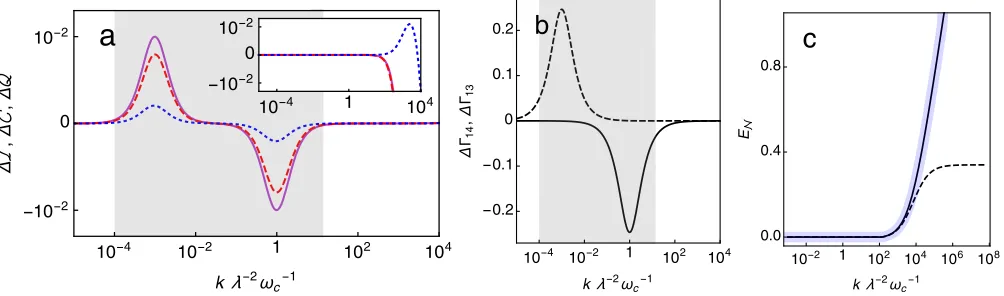
As we can see from Fig.2(a)the inter-node correlations can be both overestimated and underestimated by the global master equation whenever the secular approximation fails. In contrast, the LME assesses I faithfully. Note from Eq. (22) that the stationary covarianceshxxxcppphiandhpppcxxxhi(i.e. Γ14andΓ23) are neglected in the global approach. Indeed, it is easy to see from the corresponding Markovian Redfield equation (cf. Appendix) that these covariances are related to the excluded non-secular term at frequencyΩ+−Ω−. From Fig.2(b)we observe that thedeficitin total quantum correlations predicted by the GME

10-4 10-2 1 102 104

-10-2 0 10-2

kλ-2_ω

c-1

Δℐ

,

Δ

,

Δ

a

10-4 1 104

-10-2 0 10-2

10-4 10-2 1 102 ₁₀4

-0.2

-0.1

0 0.1 0.2

k_λ-2ωc-1

Δ

Γ14

,

Δ

Γ13

b

10-2 1 102 104 106 108

0.0 0.4 0.8

k_λ-2

ωc-1

E

c

FIG. 3. (color online)(a)Excess quantum mutual information∆I:=I(ΓG)−I(Γ)(solid purple), classical correlations∆C←:=C←(ΓG)− C←(Γ)(dashed red), and quantum correlations∆Q←=∆I−∆C←(dotted blue), as follows from the comparison of the global approach with the exact solution (see main text for definitions). The inset reproduces the main plot, benchmarking instead the local approach against the exact result. The parameters are the same as in Figs.1(b)and1(d), i.e. we work with small detuning. While the LME faithfully captures inter-node correlations in all its range of validity, the GME may both underestimate or overestimate them. In(b)the quantities∆Γ14:= [ΓG]14−[Γ]14 (solid) and∆Γ13:= [ΓG]13−[Γ]13 (dashed) are plotted for the same parameters as in (a). We see that the failure of the global approach to correctly assess these covariances (hxxxcppphi=−hpppcxxxhiandhxxxcxxxhi) explains the peaks in (a). In(c)we plot the steady state inter-node entanglement, as quantified by the logarithmic negativityENwithin the global (solid black), local (dashed black), and exact (thick transparent

blue) approaches. The observation of non-vanishing asymptotic entanglement requires large ratiosω/Tα and very large coupling strengths k. Unfortunately, this prevents entanglement from being observed in the problematic regionk/ωc.λ2. Interestingly, the LME predicts a

saturation ofEN for largek, which is anyway far beyond its range of applicability. In (c)ωc=ωh=10,Tc=1,Th=2,λ2=10−3, and Λ=103.

It is possible to split the total correlations into aquantumand aclassicalshare (blue dotted and red dashed lines in Fig.2(a), respectively). We will say that a bipartite quantum stateρρρAB has quantum correlations with respect to B if there exists no local measurement onBthat leaves the marginal of A unperturbed. This notion ofquantumnessof correlations is captured by the discordQ←₍

ρ ρ

ρAB):=S(ρρρB)−[S(ρρρAB)−inf{ΠΠΠB_j}∑jpjS(ρρρA|j)][43,44]. Given a complete set of projectors{ΠΠΠ

B j}onB, ρρρA|j:=trB{ΠΠΠB_jρρρABΠΠΠB_j}denotes the post-measurement marginal ofAconditioned on the outcome j, occuring with probability pj=tr{ΠΠΠB_jρρρAB}. Note that discord is not symmetric, i.e. the quantumness of correlations as revealed by measurements onB need not coincide with the quantumness of correlations as revealed by measurements onA.

Note as well that, due to the explicit minimization over all local measurements onB, the evaluation of Q← _{is often very}

challenging. Luckily, restricting the optimization to the set of Gaussian positive operator valued measurements makes it possible to obtain a closed formula for two-mode Gaussian states (see Ref. [45–47] for full details). The difference between the total correlations and the quantum discord is referred-to as classical correlations C←₍

ρ

ρρAB):=I(ρρρAB)−Q←(ρρρAB). As shown in Fig.2(a), both quantum and classical correlations behave very similarly to the mutual information within the global approach. This is not the case, however, for the LME [cf. inset in Fig.2(a)]: at large coupling strengths (i.e. beyond its range of validity) the local approach may overestimate the amount of quantum correlations present between the nodes, although at sufficiently large couplings, all correlations are largely underestimated.

Finally, we may want to look at the inter-nodeentanglement[48]. Entanglement is a somewhat stronger form of quantum correlation since a state can display non-zero discord and yet be unentangled, but not the other way around. In the case of two-mode Gaussian states, quantum entanglement can be gauged by the logarithmic negativityEN, which writes as [49,50]

EN(Γ):=

_∑

j

max{0,−log(2 ˜νj)}, (37)

where ˜νj are the symplectic eigenvalues of thepartially-transposedcovariance matrix ˜Γ. This is obtained fromΓ by simply changing the sign of all covariances involving e.g. the momentumpppcand either of the ‘hot’ quadratures.

The buildup of steady-state entanglement requires much larger inter-node couplingkand large ratiosωα/Tα as shown in Fig.2(c). While there is no reason for the GME not to accurately capture the entanglement ask→∞, the LME wrongly predicts a saturation in the stationary logarithmic negativity in that limit. One can obtain the correct scaling of entanglement at strong coupling from the GME which, for resonant nodes, simplifies to

EN(Γ) →

k→∞ 1 4log

2k(1−eω/Tc₎2_(1−eω/Th₎2

(1−e2ω/T¯₎2_ω2 with T¯:= T−1

c +T

−1 h 2

−1

V. CONCLUSIONS

We have studied a simple model for heat transport between two heat baths at different temperatures when weakly connected through a two-node quantum wire. Due to the weak dissipative wire-baths coupling, it is possible to address the problem via second-order Markovian quantum master equations. In particular, we consistently derived the GKLS master equation via a globaltreatment of dissipation, and found its steady state, the stationary heat currents through the wire, and the asymptotic inter-node quantum and classical correlations. For comparison, we adopted the popularlocalapproach, which addresses dissipation on each node individually (i.e. ignoring the effects of the inter-node coupling). Since our model is linear, its steady state can be obtainedexactlyby resorting to quantum Langevin equations. This provided us with means to quantitatively compare the performance of the global and the local approaches.

As expected, we found that the local approach is only valid when the internal coupling between the nodes of the wire is weak. Furthermore, as previously noted, we observed that the local approach does break the second law of thermodynamics [15], although any violations can be bounded with suitably-defined error bars within its range of applicability [18].

Interestingly, our setup allows us to consider very weak internal couplings, comparable with the dissipation strength. In this regime, the crucial secular approximation breaks down if, in addition, the nodes are nearly resonant. As a result, the predictions of the global master GME become qualitatively wrong—the magnitude of the stationary heat currents is largely overestimated, and key features of the correlation-sharing structure are not captured by the GME. On the contrary, the LME does accurately describe the stationary properties of the wire. This agrees with previous observations on the complementarity of GME and LME when describing dynamics [19]. More generally, the usage of the local approach in the treatment of heat transport through arbitrarily long harmonic or spin chains [17] may be justified provided that the internal couplings are weak enough, and always keeping in mind that the predictions of the LME should by accompanied by the corresponding error estimates [18].

In spite of these encouraging observations, the local approach should not be used lightly, especially in quantum thermody-namics. Even though the LME may be an excellent working tool that even outperforms the canonical global GKLS master equation in certain regimes, it might as well lead to qualitatively wrong conclusions,a prioriwithin its range of applicability. For instance, it has been shown that a local modelling of quantum thermodynamic cycles completely fails to account for heat leaks and internal dissipation effects [51,52] that can become dominant in the operation of the device in question. As a result, e.g. intrinsically irreversible models may be wrongly classified asendoreversible. This is a reminder that perturbative equations of motion for open quantum systems must always be handled with care.

NOTE ADDED: During the preparation of this manuscript we became aware of the related work by Patrick P. Hoferet al. [53], where local and global approach are compared in a quantum heat engine model.

ACKNOWLEDGMENTS

The authors gratefully acknowledge A. Levy, Nahuel Freitas, and Karen V. Hovhannisyan for helpful comments. This project was funded by the Spanish MECD (FPU14/06222), the Spanish MINECO (FIS2013-41352-P), the European Research Council under the StG GQCOP (Grant No. 637352), and the COST Action MP1209: “Thermodynamics in the quantum regime”.

Appendix: ThepartialMarkovian Redfield master equation

In order to compensate for the deficiencies of the GME one may simply take into consideration the problematic non-secular term corresponding to theΩ+−Ω−channel. Eqs. (9) and (11) would then need to be combined as

dOOO

dt 'i[HHHS,OOO] +

∑

α∈{c,h}ω∈{±

∑

L L Lω

α †_OOOLLLω

α− 1 2{LLL

ω α

†_LLLω α,OOO}+

+1

2

∑

α∈{c,h}

γα(Ω+)

LLLΩα− †

OOOLLLΩα+−OOOLLL Ω− α

†

LLLΩα++LLL Ω+ α

†

O O

OLLLΩα−−LLL Ω+ α

†

LLLΩα−OOO

+1

2

∑

α∈{c,h}

γα(−Ω+)

L LLΩα−OOOLLL

Ω+ α

†

−OOOLLLΩα−LLL Ω+ α

† +LLLΩ+

α OOOLLL Ω− α

† −LLLΩ+

α LLL Ω− α

†

OOO

+1

2

∑

α∈{c,h}

γα(Ω−)

LLLΩ+

α †

OOOLLLΩα−−OOOLLL Ω+ α

†

LLLΩα−+LLL Ω− α

†

O O OLLLΩ+

α −LLL Ω− α

†

LLLΩ+ α OOO

+1

2

∑

α∈{c,h}

γα(−Ω−)

L LLΩ+

α OOOLLL Ω− α

†

−OOOLLLΩ+ α LLL

Ω− α

†

+LLLΩα−OOOLLL Ω+ α

† −LLLΩα−LLL

Ω+ α

†

OOO

,

where the operatorsLLLω

α are those defined in Sec.II B.

In principle, a full set of 10 dynamical variables would be necessary to obtain all steady-state covariances. We shall choose DDD±±:=i(aaa†±aaa±† −aaa±aaa±),SSS±±:=aaa†±aaa†±+aaa±aaa±,DDD+−:=i(aaa†+aaa†−−aaa+aaa−),SSS+−:=aaa†+aaa†−+aaa+aaa−,ddd+−:=i(aaa†+aaa−−aaa+aaa†−),

sss+−:=aaa†+aaa−+aaa+aaa†−, andnnn±:=aaa†±aaa±. As it turns out, the stationary averages of the first six variables vanish (i.e. hDDD±±i=

hSSS±±i=hDDD+−i=hSSS+−i=0), so that we are left with only four relevant observables. The corresponding equations of motion

write as d~yyy/dt=B~yyy+b, where~yyy= (nnn+,nnn−,ddd+−,sss+−)T, the non-zero elements ofbare given by

[b]₁=W₋c_Ω++W₋h_Ω+ (A.2a)

[b]2=W−cΩ−+W h

−Ω− (A.2b)

[b]4= s

Ω+

Ω−

(W₋c_Ω

+tanϑ−W h

−Ω+cotϑ) + s

Ω−

Ω+

(W₋c_Ω−cotϑ−W−hΩ−tanϑ), (A.2c)

and the coefficients of the matrixBread

[B]11=W−cΩ++W h

−Ω+−W c Ω+−W

h

Ω+ (A.3a)

[B]14= 1 2[B]42=

1 2

s Ω−

Ω+

([W−cΩ−−W c

Ω−]cotϑ−[W h

−Ω−−W h

Ω−]tanϑ) (A.3b)

[B]22=W−cΩ−+W h

−Ω−−W c Ω−−W

h

Ω− (A.3c)

[B]24= 1 2[B]41=

1 2

s Ω+

Ω−

([W₋c_Ω+−W_Ωc₊]tanϑ−[W−hΩ+−W h

Ω+]cotϑ) (A.3d)

[B]33= [B]44= 1 2(W

c

−Ω−+W c

−Ω++W h

−Ω−+W h

−Ω+−W c Ω−−W

c Ω+−W

h Ω−−W

h

Ω+) (A.3e)

[B]34=−[B]43=Ω−−Ω+. (A.3f)

All the remaining coefficients vanish.

The non-zero elements of the steady-state covariance matrixΓRin the basis of the normal modes{ηηη−,ΠΠΠ−,ηηη+,ΠΠΠ+}are

[ΓR]₁₁= 1 Ω−

1 2+hnnn−i

, [ΓR]₂₂=Ω−

1 2+hnnn−i

,

[ΓR]33= 1 Ω+

₁ 2+hnnn+i

, [ΓR]44=Ω+ ₁

2+hnnn+i

,

[ΓR]₁₃= [ΓR]₃₁= 1 2√Ω+Ω−

hsss+−i, [ΓR]14= [ΓR]41=− 1 2

s Ω−

Ω+ hddd+−i,

[ΓR]23= [ΓR]32= 1 2

s Ω+

Ω−

hddd+−i, [ΓR]24= [ΓR]42= 1 2

p

Ω+Ω−hsss+−i.

(A.4)

Just like in Eq. (22), this can be rotated into the original quadratures by applying the suitable rotation matrix as defined in Eqs. (12) and (13).

Finally, the steady state heat currents obtained from the stationary solution of Eq. (A.1) can be cast as

˙ QR

c =−Q˙Rh =Ω+ h

W_Ωc₊hnnn+i −W−cΩ+(1+hnnn+i) i

+Ω−

h

W_Ωc₋hnnn−i −W−cΩ−(1+hnnn−i) i

+1 2

p

Ω+Ω−hsss+−i

h

(W_Ωc₋−W−cΩ−)cotϑ+ (W c Ω+−W

c

−Ω+)tanϑ i

. (A.5)

[1] G. Lindblad, “On the generators of quantum dynamical semigroups,”Comm. Math. Phys.48, 119 (1976).

[2] V. Gorini, A. Kossakowski, and E. Sudarshan, “Completely positive dynamical semigroups of N-level systems,”J. Math. Phys.17, 821

(1976).

[4] H. Spohn, “Entropy production for quantum dynamical semigroups,”J. Math. Phys.19, 1227 (1978).

[5] A. M¨uller-Hermes and D. Reeb, “Monotonicity of the quantum relative entropy under positive maps,”D. Ann. Henri Poincar´e18, 1777

(2017).

[6] H. Spohn, “An algebraic condition for the approach to equilibrium of an open N-level system,”Lett. Math. Phys.2, 33 (1977). [7] R. Alicki, “The quantum open system as a model of the heat engine,”J. Phys. A12, L103 (1979).

[8] R. Kosloff, “A quantum mechanical open system as a model of a heat engine,”J. Chem. Phys.80, 1625 (1984). [9] J. P. Palao, R. Kosloff, and J. M. Gordon, “Quantum thermodynamic cooling cycle,”Phys. Rev. E64, 056130 (2001). [10] R. Kosloff, “Quantum Thermodynamics: A Dynamical Viewpoint,”Entropy15, 2100 (2013).

[11] R. Kosloff and A. Levy, “Quantum Heat Engines and Refrigerators: Continuous Devices,”Anual Rev. Phys. Chem.65, 365 (2014). [12] D. Gelbwaser-Klimovsky, W. Niedenzu, and G. Kurizki, “Thermodynamics of Quantum Systems Under Dynamical Control,”Adv. At.

Mol. Opt. Phy.64, 329 (2015).

[13] S. Vinjanampathy and J. Anders, “Quantum thermodynamics,”Contemp. Phys.57, 545 (2016).

[14] J. Goold, M. Huber, A. Riera, L. del Rio, and P. Skrzypczyk, “The role of quantum information in thermodynamics—a topical review,”

J. Phys. A: Math. Theor.49, 143001 (2016).

[15] A. Levy and R. Kosloff, “The local approach to quantum transport may violate the second law of thermodynamics,”Europhys. Lett.107,

20004 (2014).

[16] J. T. Stockburger and T. Motz, “Thermodynamic deficiencies of some simple Lindblad operators,”Fortschr. Phys. , 1 (2016).

[17] H. Wichterich, M. J. Henrich, H.-P. Breuer, J. Gemmer, and M. Michel, “Modeling heat transport through completely positive maps,”

Phys. Rev. E76, 031115 (2007).

[18] A. Trushechkin and I. Volovich, “Perturbative treatment of inter-site couplings in the local description of open quantum networks,”

Europhys. Lett.113, 30005 (2016).

[19] A. Rivas, A. D. K. Plato, S. F. Huelga, and M. B. Plenio, “Markovian master equations: a critical study,”New Journal of Physics12,

113032 (2010).

[20] C. Fleming, N. I. Cummings, C. Anastopoulos, and B. L. Hu, “The rotating-wave approximation: consistency and applicability from an open quantum system analysis,”Journal of Physics A: Mathematical and Theoretical43, 405304 (2010).

[21] T. M. Stace, A. C. Doherty, and D. J. Reilly, “Dynamical Steady States in Driven Quantum Systems,”Phys. Rev. Lett.111, 180602

(2013).

[22] J. P. Santos and G. T. Landi, “Microscopic theory of a nonequilibrium open bosonic chain,”Phys. Rev. E94, 062143 (2016).

[23] A. Purkayastha, A. Dhar, and M. Kulkarni, “Out-of-equilibrium open quantum systems: A comparison of approximate quantum master equation approaches with exact results,”Phys. Rev. A93, 062114 (2016).

[24] G. Dec¸ordi and A. Vidiella-Barranco, “Two coupled qubits interacting with a thermal bath: A comparative study of different models,”

Opt. Commun.387, 366 (2017).

[25] A. G. Redfield, “On the theory of relaxation processes,”IBM J. Res. Dev.1, 19 (1957).

[26] I. de Vega and D. Alonso, “Dynamics of non-Markovian open quantum systems,”Rev. Mod. Phys.89, 015001 (2017).

[27] G. Adesso, S. Ragy, and A. R. Lee, “Continuous variable quantum information: Gaussian states and beyond,”Open Syst. Inf. Dyn.21,

1440001 (2014).

[28] P. Gaspard and M. Nagaoka, “Slippage of initial conditions for the Redfield master equation,”J. Chem. Phys.111, 5668 (1999). [29] J. Jeske, D. J. Ing, M. B. Plenio, S. F. Huelga, and J. H. Cole, “Bloch-Redfield equations for modeling light-harvesting complexes,”J.

Chem. Phys.142, 064104 (2015).

[30] H. Grabert, U. Weiss, and P. Talkner, “Quantum theory of the damped harmonic oscillator,”Z. Phys. B55, 87 (1984). [31] U. Weiss,Quantum dissipative systems, Vol. 13 (World Scientific Pub Co Inc, 2008).

[32] D. Boyanovsky and D. Jasnow, “Heisenberg-Langevin vs. quantum master equation,”preprint arXiv:1707.04135.

[33] M. Ludwig, K. Hammerer, and F. Marquardt, “Creation and destruction of entanglement by a nonequilibrium environment,”Phys. Rev.

A82, 012333 (2010).

[34] L. A. Correa, A. A. Valido, and D. Alonso, “Asymptotic discord and entanglement of nonresonant harmonic oscillators under weak and strong dissipation,”Phys. Rev. A86, 012110 (2012).

[35] A. A. Valido, D. Alonso, and S. Kohler, “Gaussian entanglement induced by an extended thermal environment,”Phys. Rev. A88, 042303

(2013).

[36] A. A. Valido, L. A. Correa, and D. Alonso, “Gaussian tripartite entanglement out of equilibrium,”Phys. Rev. A88, 012309 (2013). [37] A. A. Valido, A. Ruiz, and D. Alonso, “Quantum correlations and energy currents across three dissipative oscillators,”Phys. Rev. E91,

062123 (2015).

[38] N. Freitas and J. P. Paz, “Analytic solution for heat flow through a general harmonic network,”Phys. Rev. E90, 042128 (2014). [39] N. Freitas and J. P. Paz, “Fundamental limits for cooling of linear quantum refrigerators,”Phys. Rev. E95, 012146 (2017). [40] M. A. Nielsen and I. L. Chuang,Quantum computation and quantum information(Cambridge University Press, 2000). [41] P. Marian and T. A. Marian, “Uhlmann fidelity between two-mode Gaussian states,”Phys. Rev. A86, 022340 (2012). [42] A. S. Holevo and R. F. Werner, “Evaluating capacities of bosonic Gaussian channels,”Phys. Rev. A63, 032312 (2001).

[43] H. Ollivier and W. H. Zurek, “Quantum Discord: A Measure of the Quantumness of Correlations,”Phys. Rev. Lett.88, 017901 (2001). [44] L. Henderson and V. Vedral, “Classical, quantum and total correlations,”J. of Phys. A: Math. Gen.34, 6899 (2001).

[45] G. Adesso and A. Datta, “Quantum versus classical correlations in Gaussian states,”Phys. Rev. Lett.105, 30501 (2010). [46] P. Giorda and M. G. A. Paris, “Gaussian Quantum Discord,”Phys. Rev. Lett.105, 020503 (2010).

[47] S. Pirandola, G. Spedalieri, S. L. Braunstein, N. J. Cerf, and S. Lloyd, “Optimality of Gaussian Discord,”Phys. Rev. Lett.113, 140405

(2014).

[50] M. B. Plenio, “Logarithmic Negativity: A Full Entanglement Monotone That is not Convex,”Phys. Rev. Lett.95, 090503 (2005). [51] L. A. Correa, J. P. Palao, G. Adesso, and D. Alonso, “Performance bound for quantum absorption refrigerators,”Phys. Rev. E87, 042131

(2013).

[52] L. A. Correa, J. P. Palao, and D. Alonso, “Internal dissipation and heat leaks in quantum thermodynamic cycles,”Phys. Rev. E92, 032136

(2015).