Calculation of High-Order Virial Coefficients for the Square-Well Potential
Hainam Do,1 Chao Feng,3 Andrew J. Schultz,2 David A. Kofke,2 and Richard J. Wheatley1,*
1School of Chemistry, University of Nottingham, University Park, NG7 2RD, United
Kingdom
2Department of Chemical and Biological Engineering, University at Buffalo, The
State University of New York, Buffalo, NY, 14260-4200, USA
3Department of Computer Science and Engineering, University at Buffalo, The State
University of New York, Buffalo, NY, 14260-4200, USA
*Email: [email protected]
Abstract
1. Introduction
The pressure P of a fluid at temperature T can be expanded in powers of the number density ρ as
P
kBT =ρ+ BN(T)ρ N
N=2
∞
∑
(0)where kB is the Boltzmann constant and BN is the virial coefficient of order N.
Despite the fact that this equation of state has a well-established theoretical foundation and is important in the physical sciences, its applications are still rather limited. This is partly because high-order virial coefficients are needed to investigate the convergence properties of the series, and to improve the convergence by, for example, resummation via rational functions or other forms [1–8], but such coefficients are difficult to calculate. Much work has been devoted to the hard-sphere model, for which orders N≤10 have been calculated [9–11], before a breakthrough in the algorithm was made [12] that gave access to higher orders [12–14]. Recently, the algorithm also made possible calculations beyond N = 8 for the Lennard-Jones potential [15].
The square-well (SW) potential is perhaps the simplest model that exhibits behavior that is common to most fluids, including vapor-liquid equilibrium and a critical point. It has been employed to investigate a variety of interesting problems, including interfacial phenomena, surface adsorption, wetting and capillary condensation [16– 18]. The temperature dependence of all virial coefficients of the SW potential can be expressed in an exact closed form (polynomial) and the calculation of the virial coefficients is more tractable than other realistic potentials. The virial coefficients of the SW potential have been studied for more than half a century [19–26]. However, the maximum order attainable through calculation only reached N = 6 quite recently [26], which emphasizes the difficulties in obtaining higher order virial coefficients for model fluids in general, and for the SW potential in particular, relative to the hard-sphere case.
In this paper, we propose an efficient algorithm that enables us to obtain the virial coefficients BN(λ, f), of orders N = 5 to 9 for the three-dimensional,
separation r≤σ , E=−ε for σ <r<λσ , and E=0 for r≥λσ . The hard-core diameter is
σ
. The virial coefficients depend on the reduced well depth ε/kBT , which is represented here by f, the Mayer function evaluated in the well regionf =exp(ε/kBT)−1
(
)
, and on the reduced well width λ. The calculations cover the range 1.1≤λ≤2.0 , for which thermodynamic properties such as the critical temperatures and densities are available for comparison. The focus of this paper is primarily on method development and two similar but distinct Monte Carlo methods are discussed.2. Methods
The calculated virial coefficients are expressed in reduced form as
BN* =B
N / [B2(HS)]
N−1, where B
N(HS) is the N
th virial coefficient for the hard-sphere core, with diameter
σ
, and B2(HS)= 2π3 σ
3. As a function of f, the virial coefficients take their hard-sphere values at f =0 (no well):
BN*(λ,0)=B
N(HS) / [B2(HS)] N−1=B
N
*(HS) . Negative values of f, −1≤ f <0 , correspond to a square-step potential with positive potential energy, with f =−1
representing an infinitely high step, for which BN*(λ,−1)=λ3(N−1)B N
*(HS) . Increasingly positive values of f correspond to square-well potentials of greater well depth, and for f > fc a bulk liquid phase is possible [27], where fc=exp(1 /Tc
*
)−1
and Tc* is the reduced critical temperature.
Numerical integration (Monte Carlo) is used to calculate the virial coefficients, using the standard integral
BN(λ,f)= 1−N
N!
∫
... fB(λ,f,r N)dr2...drN
∫
(0)and a recursive method of calculation [12] is modified (see Supplemental Material [28]) to evaluate the integrand fB , which defined as
fB(λ,f,rN)= f(r
ij) ij∈G
∏
⎡ ⎣ ⎢ ⎤ ⎦ ⎥ G∑
, where G is a biconnected graph. The integrand, andobtained in closed form, for each well width considered, at all temperatures and densities for which the virial series converges. The polynomial expansion of the reduced virial coefficients is given in terms of the coefficients BN,j
* (λ ) as BN*(λ,f)= B
N,j
* (λ)
j=0
m
∑
fj (1)The upper summation limit m=N(N−1) / 2 is the number of pairs of particles. From the limiting cases above, it follows that BN,0* =B
N
*(HS) and
BN,j* j=0
m
∑
(−1)j =λ3(N−1)BN*(HS) (1)The recursive method [12] takes as its starting point the quantity exp(−E/kBT) for a
set of N particles and for all subsets thereof. For the pair-additive square-well potential, this quantity is either zero, if any hard-core overlaps occur in the (sub)set, or (f +1)p, if p pairs of particles are in the well region and the rest are outside it. The implementation of the recursive method is modified to retain this explicit polynomial dependence on (f +1) at each stage. The resulting integrand fB is integrated stochastically to give BN as a polynomial in (f +1), which is then converted to the required polynomial in f.
The computer time required for the recursive algorithm scales as 3N
N when numerical values are used, but since polynomials of order up to m=N(N−1) / 2 are required in this work, the time increases further. It is therefore highly beneficial to invoke the method on a configuration of particles only when needed. One strategy to this end is to store the integrand for re-use during the calculation for each λ and N. The integrand depends only on the graph that describes whether each pair separation is in the hard-core region, the well, or the zero-energy long-range region, and not explicitly on the particle positions within these regions. Given that there are three possibilities per pair, there is a maximum of 3m possible graphs. For N = 5 and 6 (m = 10 and 15) the number of graphs is sufficiently small that all the integrands fB can be stored when first needed, and looked up thereafter.
approaches analogous to previous work for hard spheres [12,14]. Both execute a repeated process of: (1) generating a configuration at random by placing each particle in succession relative to a previously-positioned particle, starting with the first at the origin; (2) evaluating some simple metrics for the resulting configuration to determine whether to compute fB for it; (3) if so indicated, computing fB using the recursive method, and also computing the total probability w for producing the configuration, considering how step (1) could yield it for all N! permutations of the particles; (4) incrementing an average with fB/w.
In Method A [12], the particles are placed in a chain, such that each new particle is inserted relative to the one just preceding it, with probability that is uniform within the sphere for distances r from 0 to λσ , and decreasing proportionally to r−12 for
larger distances; this probability tail is needed so that all biconnected diagrams have a nonzero chance of being produced. Dynamically generated lookup tables are used to evaluate the integrand.
For N ≥7, the invariance of the integrand to permutation of particle labels is used, giving a storage requirement of order up to 3m/N!. To exploit the permutation
This re-ordering is not fully canonical (it does not recognize the permutation equivalence of some graphs), but the number of reordered graphs that are generated is found to be less than 3m
/N! in practice. If a graph is not biconnected (where a pair with separation in the core or well region is counted as a connected pair) then the integrand is zero, and is not stored. Many graphs are never produced in practice because they are geometrically impossible (or highly unlikely) in three dimensions. If the storage space is insufficient to accommodate a few rarely generated configurations, this is also acceptable, because the time taken to apply the recursive algorithm to the unstored graphs every time they are generated is not prohibitive. However, for N = 9 the storage requirements become sufficiently large that a parallel algorithm is used. Each parallel task is assigned a similar number of biconnected canonical graphs. Each configuration that is generated is checked for biconnectivity, its total probability and canonical ordering are calculated, and these data are sent to the appropriate task for analysis. This balances the storage and processing load between the tasks, and it is found that the computer time is roughly equally divided between the generation of random chains, checking them for biconnectivity, calculating the total probability of generating the chain configurations, performing the canonical re-ordering, and computing the integrands. More details on this are given in the result section.
of whether to compute fB/w for a generated configuration is made with probability that depends on the observed variance for its bin, and other factors (with some non-zero probability to compute it regardless of its bin variance), and is adjusted to optimize the calculation [14].
The accuracy of the calculated virial coefficients depends on the quality of the random number generator used; so several different pseudo-random and quasi-random number generators are investigated for producing the random chains. Most of the results presented for Method A are produced using digit-permuted Halton numbers [29], but the Mersenne Twister [30] and random Latin Hypercube [31] methods give consistent results with similar confidence limits; for Method B, the Mersenne Twister is used exclusively.
Uncertainties represent 68% confidence intervals of the corresponding coefficient. For a given N, the coefficients BN*,j
are correlated, so the uncertainty in BN* cannot be
obtained from them via simple error propagation. Hence, the uncertainties in BN*
using Method A are computed from averages of the BN* at each temperature (f) value
reported. Calculations using Method B recorded the covariances needed to propagate the BN*,j errors to
BN, and these values are included in the SM.
3. Results and Discussions
Results for the coefficients BN,j
* with well width
1.1≤λ≤2.0 along with the
minimum uncertainty averages of the two methods are given in the SM. A comparison of the uncertainty between the two methods is also provided in this document. For completeness, formulas and results for N = 2, 3, and 4 are also included in the SM.
As outlined above, there are two limiting cases of the SW potential where data for the HS model can be extracted from the calculations: when f = 0 BN
*
(HS)=BN *(λ,0)
(
)
and −1 BN
*
(HS)=BN
*
(λ,−1) /λ3(N−1)
(
)
. These are used as a partial check on the calculated BN,j* . For the fifth virial coefficient with λ=
1.5 (Table 1), the B5,0
is 0.1102530(22), and BN*(HS) obtained using f = −1 is 0.1102517(2), which agree well with the literature value 0.11025147(6) [9]. The coefficients BN*(HS) from the
limiting case f = −1 always have better precision than those from f = 0, because the “large spheres” with diameter λσ (f = −1) are sampled better than the “small spheres” with diameter
σ
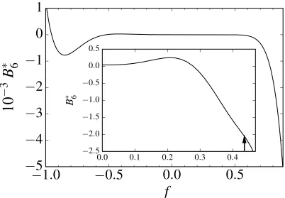
(f = 0). For N >5, there is similar agreement between the HS limiting cases and the HS data from the literature. Thus, these give confidence in the accuracy of all other BN*,j coefficients reported here.The temperature dependence of the virial coefficients can be examined by plotting BN*(λ,f) against f. This is shown in Figures 1 and 2 for B
6
*(2,f) and B
9
*(2,f) as examples. Similar Figures for other BN*(λ,f) can be generated from the BN,j
*
data given in the SM. Negative f values correspond to a square-step potential with increasing step height for more negative f, while small positive f values correspond to a SW potential at supercritical temperatures, and large positive f values correspond to low temperatures; BN*(λ,f) goes to −∞ as f approaches ∞. For N =6 and λ=
2.0
(Figure 1), the standard error in the virial coefficient is very small, which suggests that the calculated B6*(2,f) is useful for a wide range of well depths. The standard errors increase from about 1% to 10% for all well widths λ=1.1−2.0 near the
critical point between order N = 5 and 8. For N = 9, the uncertainty in B9*(2,f) (Figure 2) is more significant around the critical point, with a percentage error of ~36%.
The longest calculation, which is for B9*(1.5,f) , used a total of 5×10¹² configurations with Method A and took ~34,000 seconds real time per core when run in parallel on 1200 2.7 GHz CPU cores on a Cray XC30 supercomputer. The number of biconnected graphs found was ~ 4×10¹¹. The number of integrands (polynomials)
stored was ~ 3×10⁹, which means that the number of integrands that has to be
and ~7000 s respectively, which amounts to ~96% of the total time. The time taken to send and receive data from other processes is therefore insignificant.
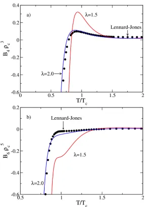
Some qualitative differences in behavior of the SW model with respect to λ can be uncovered by comparison of their temperature-dependent virial coefficients when reduced by critical properties. Figure 3 shows the temperature dependence of B4 and B6 for λ = 1.5 and 2.0, with behavior of the Lennard-Jones (LJ) model provided for reference. The value of the reduced coefficients—which represents their contributions to P/ρkBT at the critical density—for λ = 1.5 is 3.0 to 5.6 times larger (for N = 4 and 6, respectively) than that for λ = 2.0 when evaluated at their respective critical temperatures. The λ = 2.0 SW coefficients are much more in line with the behavior of the LJ model, but still the λ = 2.0 B6 contribution is 2.6 times greater than that for LJ at their respective critical points. This behavior for N = 4 and 6 is illustrative of the other coefficients as well. Accordingly, attempts to evaluate the critical properties for the SW model from these coefficients do not succeed as well as for the LJ model [5]. The use of approximants [5,7] may improve this outcome, and the coefficients reported here should be very useful in formulating such treatments.
4. Conclusion
To conclude, the algorithm developed in this work is capable of obtaining high order virial coefficients for the SW potential efficiently and accurately. It could also be applied to compute higher order virial coefficients for other discrete potential models, including the hard-sphere model. Extension to mixtures and systems of different dimensionality is straightforward.
Acknowledgement
Reference
[1] M. N. Bannerman, L. Lue, and L. V. Woodcock, J. Chem. Phys. 132, 084507 (2010).
[2] M. Ončák, A. Malijevský, J. Kolafa, and S. Labík, Condens. Matter Phys. 15, 1 (2012).
[3] N. S. Barlow, A. J. Schultz, S. J. Weinstein, and D. A. Kofke, J. Chem. Phys. 137, 204102 (2012).
[4] M. V. Ushcats, J. Chem. Phys. 141, 101103 (2014).
[5] N. S. Barlow, A. J. Schultz, D. A. Kofke, and S. J. Weinstein, AIChE J. 60, 3336 (2014).
[6] R. Bonneville, Fluid Phase Equilib. 397, 111 (2015).
[7] N. S. Barlow, A. J. Schultz, S. J. Weinstein, and D. A. Kofke, J. Chem. Phys. 143, 071103 (2015).
[8] A. J. Schultz and D. A. Kofke, Fluid Phase Equilib. 409, 12 (2016). [9] E. J. J. Van Rensburg, J. Phys. A. Math. Gen. 26, 4805 (1999).
[10] S. Labík, J. Kolafa, and A. Malijevský, Phys. Rev. E 71, 021105 (2005). [11] N. Clisby and B. McCoy, J. Stat. Phys. 122, 15 (2006).
[12] R. J. Wheatley, Phys. Rev. Lett. 110, 200601 (2013). [13] C. Zhang and B. M. Pettitt, Mol. Phys. 112, 1427 (2014). [14] A. J. Schultz and D. A. Kofke, Phys. Rev. E 90, 023301 (2014).
[15] C. Feng, A. J. Schultz, V. Chaudhary, and D. A. Kofke, J. Chem. Phys. 143, 044504 (2015).
[16] S. Hlushak, A. Trokhymchuk, and S. Sokołowski, J. Chem. Phys. 130, 234511 (2009).
[17] F. Del Río, E. Ávalos, R. Espíndola, L. F. Rull, G. Jackson, and S. Lago, Mol. Phys. 100, 2531 (2002).
[18] L. A. del Pino, A. L. Benavides, and A. Gil-Villegas, Mol. Simul. 29, 345 (2003).
[19] T. Kihara, Rev. Mod. Phys. 27, 412 (1955). [20] S. Katsura, Phys. Rev. 115, 1417 (1959). [21] S. Katsura, J. Chem. Phys. 45, 3480 (1966).
[22] J. A. A. Barker and J. J. Monaghan, J. Chem. Phys. 36, 2558 (1962). [23] D. A. McQuarrie, J. Chem. Phys. 40, 3455 (1964).
[24] E. M. Sevick and P. A. Monson, J. Chem. Phys. 94, 3070 (1991).
[26] J. R. Elliott, A. J. Schultz, and D. A. Kofke, J. Chem. Phys. 143, 114110 (2015).
[27] L. Vega, E. de Miguel, L. F. Rull, G. Jackson, and I. A. McLure, J. Chem. Phys. 96, 2296 (1992).
[28] See Supplemental Material at [URL will be inserted by publisher] for a) Tabulation of coefficients, b) Method B covariances, c) Graphical comparison of results from two methods, d) Calculation of B2, B3 and B4, e) Bin definitions for Method B, and f) Algorithm for calculation of square-well virial coefficients.
[29] E. Braaten and G. Weller, J. Comput. Phys. 33, 249 (1979).
[30] M. Matsumoto and T. Nishimura, ACM Trans. Model. Comput. Simul. 8, 3 (1998).
Figure 1. Sixth virial coefficient of λ=2.0. Inset shows an expansion of the supercritical fluid region and the arrow indicates the critical point (fc). The standard errors are smaller than the width of the lines in the plots.
−
1.0
−
0.5
0.0
0.5
f
−
5
−
4
−
3
−
2
−
1
0
1
10
−
3
B
∗
6
0.0 0.1 0.2 0.3 0.4
−2.5
−2.0
−1.5
−1.0
−0.5 0.0 0.5
B
[image:12.595.97.499.69.348.2]Figure 2. Ninth virial coefficient of λ=2.0. The standard errors are smaller than the
width of the line in the main plot. Inset shows an expansion of the supercritical fluid region with error bars denoting the 68% confidence level, and the arrow indicates the critical point (fc).
−
1
.
0
−
0
.
5
0
.
0
0
.
5
f
−
25
−
20
−
15
−
10
−
5
0
5
10
−
4
B
∗
9
0.0 0.1 0.2 0.3 0.4 0.5
−70 −60
−50 −40
−30 −20
−10
0