Beyond in phase and anti phase coordination in a model of joint action

DOI 10.1007/s00422-016-0691-9 O R I G I NA L A RT I C L E

Beyond in-phase and anti-phase coordination in a model of joint

action

Daniele Avitabile1 · Piotr Słowi ´nski2 · Benoit Bardy3,4 · Krasimira Tsaneva-Atanasova2,5

Received: 6 August 2015 / Accepted: 27 May 2016 / Published online: 8 June 2016 © The Author(s) 2016. This article is published with open access at Springerlink.com

Abstract In 1985, Haken, Kelso and Bunz proposed a sys-tem of coupled nonlinear oscillators as a model of rhythmic movement patterns in human bimanual coordination. Since then, the Haken–Kelso–Bunz (HKB) model has become a modelling paradigm applied extensively in all areas of movement science, including interpersonal motor coordi-nation. However, all previous studies have followed a line of analysis based on slowly varying amplitudes and rotat-ing wave approximations. These approximations lead to a reduced system, consisting of a single differential equa-tion representing the evoluequa-tion of the relative phase of the two coupled oscillators: the HKB model of the relative phase. Here we take a different approach and systemati-cally investigate the behaviour of the HKB model in the full four-dimensional state space and for general coupling strengths. We perform detailed numerical bifurcation analy-ses and reveal that the HKB model supports previously unreported dynamical regimes as well as bistability between a variety of coordination patterns. Furthermore, we iden-tify the stability boundaries of distinct coordination regimes in the model and discuss the applicability of our

find-B

1 _{Centre for Mathematical Medicine and Biology, School of} Mathematical Sciences, University of Nottingham, University Park, Nottingham NG7 2RD, UK

2 _{Department of Mathematics, College of Engineering,} Mathematics and Physical Sciences, University of Exeter, Exeter, Devon EX4 4QF, UK

3 _{EuroMov, Montpellier University, 700 Avenue du Pic} Saint-Loup, 34090 Montpellier, France

4 _{Institut Universitaire de France, Paris, France} 5 _{EPSRC Centre for Predictive Modelling in Healthcare,}

University of Exeter, Exeter, Devon EX4 4QF, UK

ings to interpersonal coordination and other joint action tasks.

Keywords Coupled oscillators· Dynamical system· Bifurcation analysis·Coordination regimes·Numerical continuation·Parameter dependence

1 Introduction

Many body movements are periodic in their nature [18]. For example, postural sway [2], walking [8,20], running [37], swimming [54], galloping [8,20] and juggling [58] have a cyclic pattern in the position of the end effectors or joint angles. Synchronisation is a fundamental aspect of oscillatory coordination dynamics in human and ani-mal body movements [33] and has been found in many different situations [48]. Coordination is characterised by a bounded temporal relationship created by a convergent dynamical process [26,44]. Coordination regimes depend on symmetries and couplings between oscillators. Frequency entrainment, where two oscillators adopt a central frequency, occurs even with a very weak coupling. With a relatively strong coupling or if the system is symmetrical, phase entrainment can also take place. These processes may be continuous or intermittent; that is, the phases of the two oscil-lators may also align periodically [18,35,47].

exam-ple of such behaviour is observed in team sports (competitive games) [5,10,12,15]. In many real systems, anti-phase stabil-ity coexists with in-phase stabilstabil-ity [22,33,44,56]. Previous studies address the modelling of the two coupled oscillators as a nonlinear dynamical system, the fitting of its periodic orbits to human movements [28] and the systematic analysis of the effects of linear and nonlinear terms to the observed limit cycles [4]. The observed relations between frequency and amplitude [22] as well as peak velocities [44] in many but not all [3] oscillatory movements turned out to be well represented by a hybrid oscillator [22] formed by a com-bination of Van der Pol and Rayleigh nonlinear damping terms.

A classical example of model exhibiting bistability is the so-called HKB model proposed in the seminal work by Haken, Kelso and Bunz [18,22]. The model, which was originally developed for bimanual finger coordination [30], was found to be representative of a wide range of applications in human movement [7,18], suggesting that the dynamics that it produces are somehow fundamental and make formal construct for the study of coordina-tion dynamics [32,33]. Although the model was originally developed in order to account for intra-personal phenom-ena, the same patterns have been shown to be represen-tative of both sensorimotor and interpersonal behaviours [31,49,50]. The model successfully reproduces not only the patterns of stability observed in bimanual coordina-tion experiments but also their dependence upon frequency [22]. The HKB model admits a potential function that yields the experimentally observed change in attractors’ landscapes. Furthermore, the HKB model and its stochastic extension reproduced the characteristic fluctuation increase and slowing down observed experimentally near instabili-ties [51].

The development of the HKB model has been inspired by the in-phase and anti-phase coordination dynamics observed in bimanual coordination in the context of the finger move-ments experiment [30,52,53]. Therefore, most previous research has focused on a fixed set of model parameters that guarantees the stability of these particular dynamics. Fur-thermore, significant contributions to understanding these coordination patterns (albeit in a narrow parameter range and with limiting assumptions on the parameters controlling the coupling strength) have been made for different oscillator frequencies and inputs [1,3,7,17,19,25] as well as noise in the system [9,49,50]. All previous mathematical analyses of the HKB model have focused on the relative phase dynam-ics, under the assumption that the amplitude of the coupled oscillators is constant [1,3,9,17,19,22]. Several recent arti-cles have studied the phase-approximation dynamics in the HKB model by considering the multiple stable states of the system and the ability to switch between them by chang-ing the frequency and the couplchang-ing parameters [38]. The

bifurcations leading to transitions between anti-phase and in-phase dynamics in a reduced phase approximation of the HKB model [16] have been also studied. To our knowledge, however, a bifurcation analysis of the full four-dimensional HKB model, considering all model parameters as well as general (i.e. weak and strong) coupling strengths, has not been performed. Such analysis could provide an insight into other possible qualitative behaviours that the solutions of the model might exhibit, as well as characterise the possi-ble changes in the dynamics of the solutions corresponding to any changes in the parameter values of the model. We also note recent further developments of dynamical systems’ approaches for studying sensorimotor dynamics, involving dynamical repertoires, hierarchies of timescales and struc-tured flows on manifolds [23].

Given that the HKB model is a widely accepted tool in this field, it is imperative to examine systematically all the possible coordination regimes supported by this system. In addition, classifying changes of dynamical regimes in terms of positions and velocities of the two coupled oscillators would undoubtedly shed light on the HKB model’s applica-bility to explain movement coordination in joint actions and human interactions with an adaptive virtual partner (VP)[13,34,40,59–61]. In the present paper, we take a dif-ferent approach in analysing the HKB model, as we study the full four-dimensional system of first order differen-tial equations describing the evolution of the positions and velocities of the two coupled oscillators. We begin by char-acterising the local and global dynamics of the single HKB oscillator and reveal a global transition in the model that governs the existence of periodic solutions in a range of the oscillator’s parameter values. We proceed by system-atically characterising the full HKB model dynamics not only by varying the coupling strength parameters but also the rest of the model parameters, i.e. the parameters govern-ing the sgovern-ingle oscillator’s properties. In addition to the very well-studied coordination patterns, we find a stable phase-locked solution that spans a wide range of relative phases and persists for a wide range of model parameters’ values. We also show that relaxing the constant amplitude assumption allows for much richer coordination dynamics and coexis-tence of various stable coordination attractors (multi-stability regimes).

2 Results

2.1 Intrinsic properties of the oscillator in the HKB model

dynamics exhibited by the VP [13,34,59–61]. The dynam-ics of the model is an important consideration in designing such systems and in particular for parametrising the ordi-nary differential equation that governs the behaviour of the VP. For example depending on the constraints of the experi-mental set-up, a certain range of amplitude and/or frequency for the VP periodic behaviour might be desirable. Although some properties of the HKB oscillator have been measured and studied both experimentally and analytically [28,29], the dynamics of the single HKB oscillator has not been system-atically investigated theoretically. To address this gap, we begin by examining a single HKB oscillator:

¨ x= − ˙x

αx2_+β˙

x2−γ

−ω2_x,

which could be written as a planar autonomous dynamical system of the form:

˙ x= y,

˙ y= −y

αx2_+β

y2−γ

−ω2_x,

(1)

wherex represents the position, ythe velocity,ω ∈ R+ is related to the natural frequency of the oscillator andα, β, γ ∈ Rare parameters governing the intrinsic dynamics of Eq. (1). The single HKB oscillator is a hybrid Rayleigh–Van der Pol [22] planar system, and although the analysis of planar systems of ordinary differential equations is very well estab-lished [21,27,43], it has not been applied to the single HKB oscillator model. Furthermore, whenever planar systems are coupled, they are often studied in the weak coupling limit, which we don’t require for the numerical continuation analy-sis presented here. In our analyanaly-sis, we focus on the global dynamics of the system and aim to characterise all possible dynamic states that the single HKB oscillator model sup-ports, as well as their dependence on all model parameters. System (1) admits the origin(0,0)as a trivial steady state for any parameter valueω∈R+. Givenω >0, the Jacobian matrix at the trivial equilibrium(x,y)=(0,0)is

J =

0 1

−ω2 _γ

For|γ| ≥ 2ω, the Jacobian has a pair of nonzero real eigenvalues:

λ=γ ±

γ2_−4ω2

2

Thus, the equilibrium is a stable node (sink) forγ <0 and unstable node (source) forγ >0. For|γ|<2ω, the Jacobian has a pair of complex conjugate eigenvalues of the form:

λ=γ 2 ±i

4ω2_−γ2

2

Hence, the equilibrium is a stable focus (spiral sink) for −2ω < γ < 0 and unstable focus (spiral source) for 0< γ <2ω.

Changing the value of the parameter γ near γ = 0 leads to a change in the sign of the eigenvalues’ real part, which is associated with loss or gain of stability. The sys-tem undergoes a Hopf bifurcation at γ = 0, which gives rise to oscillations. We could analytically verify further the sufficient conditions for the existence of Hopf bifurcation by showing that:

∂λr(γ )

∂γ

γ=0

= 1 2 =0,

l1(γ )|γ=0= −(α+

3βω2₎

2ω(ω2₊₁₎ =0

⇐⇒ α+3βω2=0,

whereλrandl1are the real part of the eigenvalues and the

first Lyapunov coefficient [36], respectively. The sign of the first Lyapunov coefficient [36] determines whether the Hopf bifurcation is subcritical or supercritical; hence, we are in the supercritical (subcritical) case ifα+3βω2 >0 (<0). The system (1) has a degenerate Hopf bifurcation whenα+ 3βω2=0.

0 25 2

0

ω

94.7

0 t

0.62

0 t

0.2

−0.2

x1

x1 3

−3 1

2 1

2

HB

γ

−20 20

0 2

6

0

γ

−1 1

ββ== 0−0.1

β= 0.2

HB SN

(b) (a)

(d) (c)

γ

−2 6

0

3 α_{α= 0}= 0.2

α=−1.0

max

x

(

t

)

max

x

(

t

)

max

x

(

t

)

max

x

(

t

)

HB

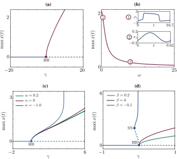
Fig. 1 Bifurcation diagrams for a single HKB oscillator.aThe trivial equilibrium becomes unstable at a supercritical Hopf bifurcation (HB) in the continuation parameterγ forω=2,α=1,β=1.bThe peri-odic orbit forγ =2 is continued in the parameterω. The lowerω, the larger the oscillations amplitude and the longer the period.c–d Contin-uations inγare repeated for various values ofαandβ. Inpanelc, for

α = −1, the periodic branch undergoes a global bifurcation (vertical asymptote), whereas inpaneld, forβ = −0.1, the Hopf bifurcation is subcritical, and the emanating branch restabilises at a saddle-node bifurcation, before disappearing in a global bifurcation.Solid(dashed) lines represent stable (unstable) states of (1)

it is important to understand where and why this singularity occurs, as it corresponds to a non-physical behaviour. Since this feature has not previously been reported in the literature on the HKB model, we present a thorough investigation of this phenomenon. In order to analyse the behaviour of the system at infinity, we employ methods presented in Chapter 3.10 of reference [46]. We start by projecting system (1) on the Poincaré sphere using the following transformation:

X= x

1+x2_+y2, Y =

y

1+x2_+y2,

Z = 1

1+x2_+y2,

which defines one-to-one correspondence between points (X,Y,Z)on the upper hemisphere S2_{withZ >0 and points}

(x,y)in the plane defined by:

x = X Z, y=

Y Z,

The points on the equator of S2correspond to points at infinity of R2. Under the transformation above, the HKB oscillator on S2withZ >0 is given by:

˙ X= Y

Z2

αX3_{Y+βX Y}3_+Z2 _{−γX Y+(ω}2_−1)X2₊₁

˙ Y = 1

Z2

(Y2−1)Y(αX2+βY2)

+Z2 Y(−γ (Y2−1)−X Y)+ω2X(Y2−1) ˙

Z = Y Z

αX2Y +βY3+Z2 (ω2−1)X−γY

(2)

System (1) has eight equilibria on the equatorX2+Y2=1 of S2(see Theorem 1 from Chapter 3.10 of [46]) that repre-sents the limitx,y→ ∞. In general, the equilibria are given by the solutions of the following equation:

(a)

α=−1, β= 1, γ= 2.6

(b)

α=−1, β= 1, γ= 3.6586

(c)

α=−1, β= 1, γ= 4

(d)

α= 1, β=−0.1, γ=−0.09

(e)

α= 1, β=−0.1, γ=−0.022618

(f)

α= 1, β=−0.1, γ= 0.5

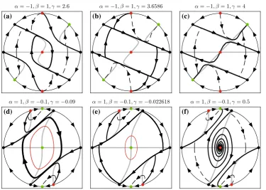
Fig. 2 Global phase portraits of the system Eq. (2), projected on the (X,Y)-plane, for different parameters values.Green dotsindicate sta-ble equilibria;red dotsindicate unstable equilibria;black dotsindicate equilibria of a saddle type;red lineindicates unstable periodic orbit;

thick black linesindicate heteroclinic connections between different

equilibria or between equilibria and stable periodic orbits;grey lines indicate nullclines;dashed linesexamples of trajectories;arrows indi-cate direction of the flow (colour figure online)

wherePmandQmare homogeneousm-th degree polynomi-als inxandy according to the following representation of the system (1):

˙

x =P(x,y)=P1(x,y)+ · · · +Pm(x,y)

˙

y=Q(x,y)=Q1(x,y)+ · · · +Qm(x,y)

(4)

In our case, the highest degree homogeneous polynomials are:

P3(x,y)=0

Q3(x,y)= −αx2y−βy3

(5)

Hence, all equilibria at the equator are the solutions of the following system of equations:

X2+Y2=1

X Q3(X,Y)−Y P3(X,Y)= −αX3Y −βY4=0

(6)

and are given by:

X =0, Y = ±1,

X = ±1, Y =0,

X = ± √

α √

α−β, Y = ± √

β √

β−α.

(7)

The flow between the nodes is determined using the fol-lowing equation (see Theorem 1 from Chapter 3.10 of [46]):

Gm₊1=cosθQm(cosθ,sinθ)−sinθPm(cosθ,sinθ)=0,

(8)

whereθis an angle along the equator.

The flow between the equilibria on the equator of the Poincaré sphere is counterclockwise ifGm₊1>0 and

clock-wise where Gm₊1 < 0. We find that only the equilibria

X = 0,Y = ±1 are hyperbolic. They are stable nodes for β < 0 and are unstable nodes for β > 0. The other six equilibria as given in (7) are non-hyperbolic. We estab-lished their types by combining information gathered from the flow on the equator and from numerical integration of the transformed system (2). We summarise our findings in two representative cases in which, as the parameterγ increases, the period and amplitude of the stable periodic orbit grows to infinity exponentially fast and the periodic orbit disappears. More specifically, at the critical valueγ∗, the stable periodic orbit becomes a heteroclinic cycle connecting four equilibria of saddle type at the equator on the Poincaré sphere.

shows the transition occurring asγ is varied in the bifurca-tion diagram of Fig.1c; and Fig.2d–f, forα=1, β= −0.1 shows the transition occurring asγ is varied in the bifurca-tion diagram of Fig.1d. In both cases, the disappearance of the stable limit cycle solution in the model is due to the same mechanism. However, depending on the signs of the parametersα, β, different invariant objects are involved in the transition. Panels (a–c) in Fig. 2 show that there are two types of connecting orbits in the phase space of the HKB oscillator. The first type connects the unstable equilibria(0,±1)(red dots) with the saddle points(±1,0) (black dots) and the second connects the saddle points (∓√α/√α−β,±√β/√β−α)(black dots) with the sta-ble periodic orbit surrounding the unstasta-ble equilibrium at the origin (0,0). As the parameter γ increases, the two types of connections become tangent and the periodic orbit stretches along theX axis as depicted in panel (b) for value ofγ = 3.65860608978 (just before the transition). At the critical value,γ = γ∗, the periodic orbit becomes a het-eroclinic cycle connecting four saddle equilibria. After the transition, the heteroclinic cycle disappears and the global phase portrait changes. In panel (c), we show that after the transition there are connections between the saddle points (∓√α/√α−β,±√β/√β−α) and the stable equilibria (±√α/√α−β,±√β/√β−α), and between the saddle points(±1,0) and the unstable equilibrium at the origin (0,0). In this case, the single HKB oscillator has stable periodic solutions only for γ ∈ (0, γ∗). Panels (d, e) in Fig.2 demonstrate that, for α = 1, β = −0.1, in addi-tion to the stable periodic orbit there is also an unstable periodic orbit (red loop) surrounding the stable equilibrium at the origin(0,0)(green dot). Although unstable periodic orbits could not be observed experimentally, such objects are important from dynamical systems point of view. For example, in this case the branch of unstable periodic orbits forms the boundary between the basins of attraction of the coexisting stable equilibrium and stable periodic orbit for γ ∈ (γSN, γ∗)(see Fig. 1d). Irrespective of the presence

of unstable limit cycle, we find again two types of con-necting orbits in the phase space for γ < γ∗ as shown in panel (d). The first type connects the unstable equilibria (∓√α/√α−β,±√β/√β−α)(red dots) with the saddle points (±√α/√α−β,±√β/√β−α) (black dots). The second type connects the saddle points(±1,0)(black dots) with the stable periodic orbit. Here we observe again that the connections become tangent to the periodic orbit, as it stretches along theX-axis growing into a heteroclinic cycle between four saddle equilibria (black dots) forγ =γ∗, as depicted in panel (e) whereγ = −0.022618 (just before the transition). After the transitionγ > γ∗, the heteroclinic cycle disappears and the invariant objects of the system recon-nect. This, however, occurs in a different manner compared to the case presented in panels (a–c). The saddle equilibria

(±1,0)are now connected with stable nodes (0,±1)and the unstable periodic orbit is connected to the saddle points (±√α/√α−β,±√β/√β−α). In panel (f), we show the phase portrait forγ =0.5, which illustrates the connections after the unstable periodic orbit disappeared in a subcritical Hopf bifurcation (at γ = 0, compare with Fig.1). In this case, the single HKB oscillator has stable periodic solutions only forγ ∈(γSN, γ∗).

2.2 Bifurcation analysis of the full HKB model

2.2.1 Full system model equations

Previous analysis of the HKB model has focussed on the dynamics of the relative phase that is given by the differ-ence of the two oscillators’ phases. However, in applications involving VP interaction environments [13,60,61], other properties of the HKB model dynamics become crucial. Such properties include the amplitude and phase of the oscillatory solutions, as well as their existence, parameter dependence and stability. In order to address these questions, we focus below on the full HKB system. The original HKB model evolves in time (measured in seconds) according to a set of nonlinear differential Equations [22]:

¨ x1+ ˙x1

αx2

1+βx˙12−γ

+ω2

x1=I12(x˙1,x˙2,x1,x2)

¨ x2+ ˙x2

αx2

2+βx˙22−γ

+ω2

x2=I21(x˙1,x˙2,x1,x2),

(9)

wherex1andx2represent the position of the two agents’ end

effectors and

I12(x˙1,x˙2,x1,x2)=(a+b(x1−x2)2)(x˙1− ˙x2)

I21(x˙1,x˙2,x1,x2)=(a+b(x2−x1)2)(x˙2− ˙x1), (10)

are coupling functions with coefficientsa,b∈R. The above system of two coupled second order ordinary differential equations (ODEs) (9) can be written as a four-dimensional autonomous system of first order ODEs:

˙ x1=y1

˙ x2=y2

˙

y1=(a+b(x1−x2)2)(y1−y2)

−(y1

αx₁2+βy12−γ

+ω2_x

1)

˙

y2=(a+b(x2−x1)2)(y2−y1)

−(y2

αx2

2+βy22−γ

+ω2

x2), (11)

system has a four-dimensional state space [7]. The parame-terω(commonly referred to aseigenfrequency) defines, in conjunction withα, βandγ, the intrinsic dynamics of the two coupled oscillators. The oscillators’ positions and velocities are coupled via the parametersaandb, commonly referred to ascoupling strengths. The HKB model behaviour then depends on the intrinsic dynamics parameters as well as the coupling strengths. Although coordination/synchronisation in system (11) emerges as a consequence of coupling, its dynamics (i.e. number, type and stability of coordination pat-terns) depends not only on the nature of the coupling but also on the intrinsic properties of each coupled oscillator. In the HKB system (11), both the intrinsic dynamics and the cou-plings are highly nonlinear, opening up the possibility of obtaining multi-stability and hence multi-functionality.

2.2.2 Coordination regimes in the HKB model

In this section, we study the existence and stability of the possible coordination regimes in the full HKB model (11) by conducting a systematic analysis in all model (control) parameters. The numerical bifurcation analysis is carried out using numerical continuation in AUTO [11]. We setNTST= 50,NCOL =4 for the mesh, andEPSL= 10−9,EPSU = 10−9 for the tolerances of the Newton solver. We perform time-stepping simulations of the model (11) in MATLAB [39], using theode45solver with default numerical settings. In the simulations presented below, we use the following typical intrinsic dynamics parameter values as default,α= 1, β=1, γ =1 andω=0.2, unless otherwise stated in the figure legends.

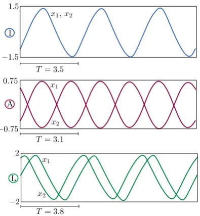
In agreement with previously performed analysis on the HKB relative phase dynamics [1,3,9,17,19,22], we confirm existence and study the stability of the well-characterised in-phase and anti-in-phase oscillatory solutions. Moreover, we find a new family of stable periodic phase-locked solutions char-acterised by relative phase in the interval(0◦,180◦). These solutions are found to be stable in a wide range of parame-ter values. We note that this family of solutions is unstable for the commonly used set of model parameters based on [22]. Examples of the three solution types described above are plotted in Fig.3. We show how such solutions are born when we varyγ for various combinations of the parame-tersa andb in the bifurcation diagrams of Fig. 4, whose branches are colour-coded as in Fig.3. Here and henceforth, we use subscripts I, A, L (or combinations thereof) to indi-cate bifurcations occurring on solution branches of in-phase, anti-phase and phase-locked solutions, respectively. We also keep the corresponding colour-code convention for branches of solutions and solutions profiles of in-phase, anti-phase and phase-locked type.

In-phase and anti-phase coordination regimes are born via Hopf bifurcations (HBI, HBA) of the trivial steady state. In

−1.5 1.5

T = 3.5

x1,x2

−0.75 0.75

T = 3.1

x1

x2

−2 2

T= 3.8

x1

x2 I

A

L

Fig. 3 Examples of stable in-phase (I), anti-phase (A) and phase-locked (L) solutions. Solutions and parameter values are also indicated in the bifurcation diagrams of Fig.4

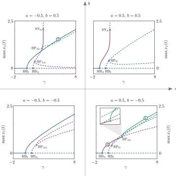
the first quadrant (where the coupling strength parameters are both positive), anti-phase coordination is the only stable state: a branch of unstable in-phase solutions is born at HBI

and bifurcates at a symmetry-breaking bifurcation, BPII,

giv-ing rise to a secondary branch of unstable in-phase solutions where the oscillation amplitudes for agent 1 and 2 differ. In the third quadrant (where the coupling strength parameters are both negative), the scenario is specular: in-phase oscilla-tions are now stable, while anti-phase soluoscilla-tions are unstable and bifurcate at BPAA. In the first and third quadrants of the

(a,b)-plane (a =0.5,b =0.5 anda = −0.5,b = −0.5, respectively), there are no branches of phase-locked solu-tions.

Phase-locked coordination regimes arise in the second and fourth quadrants of the(a,b)-plane, at symmetry-breaking bifurcations of anti-phase solutions (BPAL). Phase-locked

solutions are found to be always stable (unstable) in the fourth (second) quadrant. We note that, in these quadrants, the cou-pling non-linearities I12 and I21, as functions of x1−x2,

per-HBI HBA

BPAA

BPAL

SNA

0 2.5

max

x1

(

t

)

γ

−2 8

HBI

HBA

BPII

SNA

2.5

0

max

x1

(

t

)

γ

−2 8

HBA HBI

BPII

BPAL

2.5

0

max

x1

(

t

)

γ

−2 8

HBI HBA

BPAA

0 2.5

max

x1

(

t

)

γ

−2 8

a b

a= 0.5,b= 0.5

a= 0.5,b=−0.5

a=−0.5,b=−0.5

a=−0.5,b= 0.5

L

A I

Fig. 4 Representative bifurcation diagrams in the parameterγ for all possible combinations of coupling strengths,aandb.Solid(dashed) lines represent stable (unstable) states of (11)

−3 3

b

−1.5 1

γ

HBA HBI BPII

BPAL SNA FH

S

A

L

HBA SNA BPAL BPAA

γ

−1 4

−2 2

a

HBI BPII

I S

A

(b) (a)

BPIL

Fig. 5 Two-parameter continuations of bifurcations occurring in

Fig.4.PanelaWe fixb = 0.5 and continue in the(γ,a)-plane the

bifurcations of thetop panelsof Fig.4;shaded areasrepresent regions of stability for steady states (S), anti-phase (A) and in-phase (I) periodic

solutions.PanelbWe fixa=0.5 and continue in the(γ,b)-plane the bifurcations in the right panels of Fig.4; stable phase-locked solutions are indicated by (L)

formed so as to show how the solution landscape changes as we pass from the first to the second quadrant (continuation in (γ,a)-plane) and from the first to the fourth quadrant

cen-−4 4 0

3.5

max

x3

(

t

)

HBA

BPAA

BPAL

BPIL

a

Fig. 6 Continuation in the parametera, forb = −0.5 andγ = 1, ω=2,α=β=1. The branches show that, with suitable combination of the parameters, it is possible to have stable in-phase, anti-phase and phase-locked oscillations by varyinga.Solid linesrepresent stable and

dashed linesunstable states of (11)

tre is at γ = 0, a = 0: at this point, the eigenvalues of the linearised Jacobian at the trivial state(x1,x2,x3,x4)=

(0,0,0,0)are purely imaginary, equal to ±2i, each with multiplicity 2, corresponding to eigenvalues(0,∓i/2,0,1) and(∓i/2,0,1,0). For low positive values of the damping γ, the system supports stable in-phase solutions (for nega-tive values ofa) and stable anti-phase solutions (in a wedge delimited by the locus of SNAand BPAA). In a sizeable region

of parameter space, stable in-phase and anti-phase solutions coexist (see intersection between magenta- and blue-shaded areas). We note that the original set of parameter values based on [22] could be found in this region.

In the(γ,b)-plane, the organising centre is a fold–Hopf bifurcation aroundγ = −1,b≈1.625 (FH in Fig.5) where the locus of saddle nodes of the anti-phase solutions, SNA,

collides with the locus of Hopf bifurcations HBA. In this

region of parameter space, phase-locked solutions are found for sufficiently high damping and sufficiently negative val-ues ofb. It should be noted, however, that phase-locked and anti-phase oscillations do not coexist for the default choice of intrinsic dynamics parameter values. As it can also be ver-ified analytically, the locus of bifurcations HBA and HBB

of the stationary steady state do not depend onb. It should be also noted that, for suitable combination of the parame-ters, it is possible to visit stable in-phase, anti-phase and phase-locked oscillations by varyinga. An example of con-tinuation inaforb= −0.5 andγ =1,ω=2,a =b =1 is depicted in Fig.6. It can be clearly seen in the inset of Fig.6that, asaincreases, the stable in-phase coordination regime (characterised by relative phase 0◦) loses stability; then, a phase-locked coordination regime emerges (ranging over relative phases in(0◦,180◦)in a continuous fashion) and eventually a stable anti-phase coordination regime

(charac-ϕ1−ϕ2

a

−0.1 0.25

a

−0.1 0.25

0 0.03

0 0.04

0 0.07 0 0.18

U(0.05,0.2)

N(0.075,0.05)

(a)

(b)

0 π

ϕ1−ϕ2

0 π

Fig. 7 Distribution of the phase difference betweenx1(t)and x2(t)

(left panels) obtained when the control parametera is randomly

dis-tributed (right panels) with values close to the inset of Fig.6.aThe parametera is sampled from a uniform distribution (left) and 2000 independent simulations are performed; the histogram for the relative phaseϕ1−ϕ2is bimodal and sharply peaked around 0◦and 180◦, with a small but nonzero probability of finding an intermediate phase lag.b

The experiment is repeated with a normal distribution, which causes a third peak to develop around 90◦in the distribution for the phase lag; the latter peak is inherited from the distribution of the control parameter a

terised by relative phase 180◦) is established. The bifurcation diagram implies that, in an experimental set-up whereawere to be assigned randomly, we would observe trajectories with relative phases distributed in the interval(0◦,180◦), and with peaks at 0◦and 180◦. To verify this prediction, we performed an uncertainty quantification study, in which a is assigned randomly, near the inset of Fig.6, and histograms of relative phases betweenx1(t)andx2(t)are computed a posteriori. In

Fig.7a, we perform 2000 independent simulations, wherea is sampled from the uniform distribution between 0.05 and 0.2 and plot the resulting phase lag histogram: the distribu-tion for the phase differenceϕ1−ϕ2(right) is bimodal and

sharply peaked around 0◦and 180◦, as expected, with a small but nonzero probability of finding an intermediate phase lag. The likelihood that experiments display such intermediate relative phases is deeply affected by the distribution of a: if we pass from a uniform to a normal distribution fora, (Fig.7b), the resulting phase lag distribution develops also a peak around 90◦, which is inherited from the parameter distribution.

L

A

1 10

0 3.5

ω

max

x1

(

t

)

L2

L1

L2

x1

x2

0 1.9

t

0 1

L1

0 1

x2

x1

0 1.9

t

I

Fig. 8 Continuation of in-phase, anti-phase and phase-locked solu-tions in the frequencyω. Solutions behave similarly to the single HKB oscillator case (Fig.1b), except they have various phase behaviours. The branch of phase-locked solutions undergoes a series of saddle-node bifurcation, giving rise to stable solutions in which the phase difference

is reversed (see solutions profiles L1_,2). We note that the branches in this figure do not coexist, as they are found in different regions of para-meter space:α=β=1 anda= −0.5,b= −0.5,γ =5 (in-phase), a =0.5,b = −0.5,γ =1.2 (anti-phase) anda =0.5,b = −0.5, γ =6.2 (phase-locked)

this case the changes in the oscillation patterns occur to both agents, with various phase differences. The branch of phase-locked solutions undergoes a series of saddle-node bifurcations, giving rise to stable solutions in which the phase difference is reversed (see solutions profiles L1,2in Fig.8).

Finally we investigate the impact of intrinsic oscillator dynamics on the collective behaviour of the HKB model by performing bifurcation analysis in the intrinsic dynam-ics parametersαandβ. Instead of presenting two-parameter bifurcation diagrams for different cases, we report here only notable examples of our computations (see Figs.9and10a). The bifurcation structures found in these cases have com-mon traits with the ones discussed above for the coupling strengths parametersa andb, that is, the trivial steady state undergoes Hopf bifurcations to anti-phase and in-phase peri-odic states, and various symmetry-breaking bifurcations give rise to phase-locked solutions. Interestingly, when varyingα andβ we could find period-doubling cascades, which are found robustly whenα andβ have opposite signs, as evi-denced in Fig.9a, whereα= −0.5,β =0.5, and Fig.10a, whereα=0.5,β = −0.05. Representative stable solutions on the period-doubling cascade are also shown in Fig.10a.

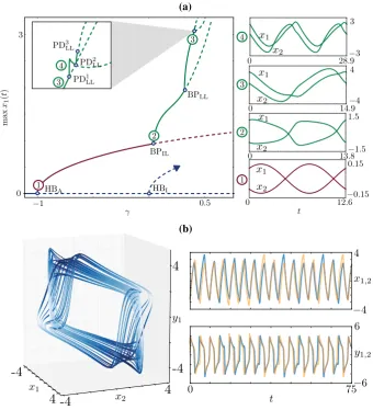
Using direct numerical simulations we explored the sys-tem behaviour close to the period-doubling cascade, finding chaotic regimes (see Fig.10b) in which the solution remains bounded and features sudden erratic phase transitions, dur-ing which the agents alternate as leaders and followers. In this regime, the velocitiesy1andy2undergo fast switches.

The existence of such complex solutions is perhaps not sur-prising from a dynamical systems viewpoint; however, the behaviour described above has not been reported nor

inves-γ

−2 4

0

max

x1

(

t

)

4

HBA HBI

BPIL

PD1

LL

PD2

LL

PD3

LL

PD4

LL

PD5

LL

α=−0.5,β= 0.5

(a)

(b)

HBAHBI

BPII

BPAL

γ

−2 8

α= 0.5,β= 0.5

max

x1

(

t

)

2.5

0

Fig. 10 Period-doubling cascade.aBranch with period-doubling cascade and stable non-trivial periodic solutions. We plot one period of several stable solutions along the branch, whereas we omit the unstable branch emanating from HBI. Solutions feature increasing solution periods,

T1≈12.6,T2≈13.8,

T3≈14.9,T4≈28.9,

corresponding toΩ1≈0.500,

Ω2≈0.455,Ω3≈0.422,

Ω4≈0.217, respectively. Parametersω=0.5,a=0.5, b= −0.5α=0.5 and β= −0.05.bAttractor found forγ=3.42; the coordination regime shows erratic phase changes, during whichx1andx2 alternate in the leading position. This regime involves fast velocity switches, as evidenced by the time traces ofy1andy2.

Solid linesrepresent stable and

dashed linesunstable states of

(11)

-4

4

4

-4

x2

y1

-4

4

−4 4

x1,2

6

−6

y1,2

0 75

t

(b)

HBA

BPIL

BPLL PD1

LL PD2 LL

1

−1 0.5

γ

max

x1

(

t

)

0 3

HBI 3

4

2

3 PD3

LL

x1 x2 0

0.15

−0.15 12.6

t

4 1

0 .−94

4 x1

x2

3 1

0 .8

1.5

−1.5 x1

x2

8 2

0 .−93

3 x1

x2

1 2 3 4

(a)

tigated previously, and can be used to model experiments where the movement coordination is irregular in nature. Last but not least, knowledge about the existence of such solutions is critical when designing virtual player interaction environ-ments [34,59–61] and/or planning human dynamic clamp experiments based on the HKB model [13].

2.2.3 Bistability and hysteresis

In this section, we explore further the dependence of the HKB model dynamics on the intrinsic properties of the cou-pled oscillators. In suitable regions of parameter space we find coexisting stable periodic states characterised by dif-ferent relative phases or phase lags. In Fig.11a, we run a continuation similar to the ones presented above, but we setα = −1.7. The branches of this bifurcation diagram are qualitatively similar to the ones of the previous sec-tions; however, the in-phase periodic branch originating at the Hopf bifurcation HBI undergoes a symmetry-breaking

bifurcation (BPIL). Such branch is initially unstable,

under-goes 2 other symmetry-breaking bifurcations, restabilises at a

saddle-node bifurcation and then features a period-doubling cascade. The stable portion of this branch (solid green branch between SNLand PDLL) coexists with a branch of stable

anti-phase solutions originating from the trivial state at HBA(red

branch).

HBA HBI

BPIL

BPLL

BPLL

SNL

SNL

PDLL

PDLL

BPAL

max

x3

(

t

)

0 5

γ

−2 8

2

2.8

SNL

SNL

PDLL

PDLL

1.5 3

2.5 4

0.9 1.7

max

x1

(

t

)

ω

2.3 2.5

ω

2.3 2.5−3.2

−1.2

ϕ1−ϕ2

(a) (b)

(c) (d)

Fig. 11 Bistability and hysteresis between anti-phase and phase-locked solutions.aThe in-phase branch (blue) undergoes a symmetry-breaking bifurcation (BPIL) and the resulting unstable phase-locked branch, featuring two further symmetry-breaking bifurcations (BPIL), restabilises at a saddle-node bifurcation, before a period-doubling cas-cade takes place. A stable portion of the phase-locked branch (solid

green linebetween SNLand PDLL) coexists with the anti-phase branch

originating at HBI(solid red branch). Parameters:a=0.5,b =0.5,

ω=3,α= −1.7,β=0.5.bWe repeat the experiment forω∈ [2,2.8] and plot stable branches to highlight the bistability region.cωis varied by continuation and by quasi-static sweeps in direct numerical sim-ulations (blue dots), forγ = 1.7; the time simulation follows the phase-locked branch up to the saddle node atω≈2.4, where an abrupt and hysteretic transition to an anti-phase solution is observed.dPhase lag during numerical simulation inc(colour figure online)

leads to transition from anti-phase to in-phase coordination. In the parameter regime described above, an increase in fre-quency leads to transition from phase-locked to anti-phase coordination behaviour.

To illustrate the dynamical switch between solution types, we perform time-stepping simulations in which the eigen-frequencyωis varied quasi-statically and compare with the bifurcation analysis. In Fig.11c, we continued an anti-phase (red) and phase-locked (green) solution forγ =1.7,ω=2.3 in the parameterω; the phase-locked branch destabilises at a saddle-node bifurcation, whereas the anti-phase branch remains stable forω∈ [2.3,2.5]. We then initialised a time simulation on the phase-locked branch (blue dots in Fig.11c) and changed ω in slow increments (from ω = 2.3 up to ω = 2.5) followed by small decrements (from ω = 2.5 down toω=2.3). The time simulation shows an abrupt and hysteretic change in the solution type. This could be further appreciated in Fig.11d where we plot the time simulation using the phase lagϕ1−ϕ2. Thex2is delayed with respect

tox1, with an initial phase lagϕ1−ϕ2≈90◦; whenω≈2.4,

we observe a transition to an orbit withϕ1−ϕ2≈180◦

(anti-phase solution).

2.2.4 Effect of heterogeneity in eigenfrequencies on the coordination regimes

In the computations shown so far, the two oscillators possess a common eigenfrequencyω. In order to study the effect of heterogeneities on coordination, we introduce two parame-tersω1,ω2, then fixω1to the nominal value ω1 = 2 and

use the ratioω1/ω2as a continuation parameter. The

differ-ence in eigenfrequencies introduces a heterogeneity in the system and has the potential to turn in-phase solutions into phase-locked solutions and vice-versa. In order to illustrate this idea, we performed bifurcation analysis in the parame-terω1/ω2investigating the in-phase solutions which exist for

Fig. 12 Phase difference between periodic solutionsx1(t) andx2(t)as a function of the ratioω1/ω2.aA stable solution on the in-phase branch in the fourth quadrant of Fig.4is continued inω1/ω2.bThe continuation is repeated starting from a solution on the

phase-locked branch in the second quadrant of Fig.4. In both cases, heterogeneity in the eigenfrequencies impacts the phase lag of the solution.c

When the ratioω1/ω2is modulated with a slowly varying sinusoidal function, the actors alternate in the leading position with hysteretic cycles, which follow the branches in theinset ofband jump at the

corresponding saddle-node bifurcations.dWe perform an experiment similar to the one in Fig.7; when the parameter ω1/ω2is drawn randomly near

theshaded areainbfrom a

uniform (blue) or a normal (red) distribution, the resulting phase lag distribution is bimodal, with peaks at±57.30◦, as predicted by the bifurcation diagram inb

and by the parameter sweep inc

(colour figure online)

ω1/ω2

1

0.9 1.1

ϕ1−ϕ2

ω1/ω2

1

0.5 1.5

ϕ1−ϕ2

SN

SN

SN

SN

SN I I

a=−0.5, b= 0.5, γ= 6.94 a= 0.5, b=−0.5, γ= 18.61

(b) (a)

π

−0.4π

0.4π

−0.4π

ω1/ω2

0.5 −1.5

1.5

ϕ1−ϕ2

1.5

(c)

(d)

0.04 0.07

ϕ1−ϕ2

0.4 0

−1.5 1.50

ω1/ω2

U(0.5,1.6)

1.6 N(1,0.15)

which we reported above fora >0 andb<0 (see Fig.4). In Fig.12, we initialise the continuation with an in-phase and a phase-locked periodic solution. We plot the bifurca-tion diagram in terms of the phase lag (measured in radians), by computing the approximate phases timesϕi =ti/T, for i =1,2, wheretiis the time at which the orbitxi(t)attains its maximum andTis the solution period. Fig.12a depicts a sta-ble, initially in-phase, solution atω1/ω2=1 that turns into a

phase-locked solution asω1/ω2is increased/decreased,

los-ing stability at saddle-node bifurcation. In Fig.12b, we show how the phase lag is reduced when the frequency ratio is var-ied and an in-phase (albeit unstable) solution is eventually attained, before a new phase-locked solution arises.

The bifurcation structure in Fig.12b implies that hystere-sis between phase-locked solutions with opposite phase lags (relative phases) is possible in the model. To illustrate this, we perform time-stepping simulations in which the ratio is varied quasi-statically asω1(t)=ω2(t)[1+sin(0.005t)]and

also in the case of randomly assigned frequency ratioω1/ω2:

when the value of this parameter is drawn randomly (close to the hysteretic region) from a uniform or a normal distri-bution, the resulting phase lag distribution is bimodal, with peaks at±57.30◦, as predicted by the bifurcation diagram in Fig.12b and by the parameter sweep in Fig.12c.

3 Discussion

In this paper, we have systematically investigated the dynam-ics of the HKB model in the state space spanned by the position and velocities of the coupled oscillators. Further-more, we go beyond the weakly coupled regime and consider the coupling strength parameters as generic. We show that stable periodic solutions in the single HKB oscillator model are born via a Hopf bifurcation as the damping parameterγ becomes positive. Furthermore, we reveal that under certain intrinsic oscillator properties the periodic solutions of the single HKB model could disappear via a heteroclinic cycle, associated with rapid increase in the magnitude of the state variables. Although such behaviour cannot be observed in a physical system, it can have significant consequences for the design and development of the virtual players. Bifurcation analysis of the full four-dimensional HKB model reveals a variety of different coordination dynamics. Attractors at a constant relative phase of 0◦ (in-phase) and/or 180◦ (anti-phase) are born via Hopf bifurcations detected in the damping parameterγ. We find symmetrical attractors of phase-locked solutions at intermediate values of relative phase (between 0◦ and 180◦), which increase or decrease gradually as γ is increased. We demonstrate that the phase-locked solu-tions are born in a symmetry-breaking bifurcation of periodic orbit in which the anti-phase periodic attractor loses sta-bility as the damping parameterγ is varied. Changing the sign of the coupling strengths has the effect of shifting the attractors by 180◦, thus changing the phase that remains sta-ble at high frequencies, from 0◦to 180◦or vice-versa. We also show that change in the intrinsic oscillators’ properties (i.e. varying the parameterα) can lead to complex dynam-ics mediated via a period-doubling cascade. Furthermore, different intrinsic dynamics can also bring about a variety of bistability modes, which are different that the type of bistability described in the original HKB model study [22]. Finally we consider a case of a heterogeneity in the system by introducing difference in the eigenfrequency of the coupled oscillators. We demonstrate how this results in bistability and hysteresis. Our uncertainty quantification simulations pre-sented in Fig.12d confirm that in the case of heterogeneous oscillators hysteresis loops and phase-locked coordination modes should be expected in experiments, as suggested in [2]. What is more, existence of such hysteresis loop pro-vides an excellent opportunity for a quantitative experimental

validation of the HKB model using two heterogeneous cou-pled oscillators, e.g. by putting weights on body parts as suggested in [2] or by using heterogeneous pendula as in [50].

In a large number of multi-stable examples observed experimentally, the patterns of stability change under dif-ferent conditions. Bimanual finger coordination is bistable at low frequencies, but above a critical frequency the anti-phase pattern is no longer sustainable [22]. Similarly postural sway is bistable at low frequencies (20◦and 180◦), but the phase-locked (20◦) mode looses stability at high frequencies or when other behaviours, such as reaching, are incorporated in the task [2]. These transitions between stable states, and par-ticularly the loss of stability of the anti-phase mode at high frequencies, appear to be a fundamental feature of human coordination [33]. The hypothesis that these real-world pat-terns and transitions between them are emergent phenomena due to a self-organised dynamical system are substantiated by experimental results such as critical fluctuations, critical slowing down and hysteresis between modes [2,18,51]. In this paper, we make the first step towards identifying para-meter regimes and dynamics that would allow to model a variety of different experimental observations using the same modelling framework.

attrac-tions to in-phase or anti-phase were observed among most dyads with the player vs. player dyads tending on balance to demonstrate less pronounced attractions or repulsions to certain relative phases than the player–opponent dyads [5,15]. Interpersonal coordination tendencies of 1-vs-1 sub-phases were investigated in [12]. The experimental results presented in Fig. 2 in [12] could be, for example, quali-tatively accounted for by the type of coordination stability dependence on the coupling parameterafound in the HKB model. Specifically (see Fig.6for b = −0.5 and γ = 1, ω = 2, α = β = 1), as the coupling strength between the velocity components of the two oscillators increases, the stable coordination regime exhibited by the HKB model undergoes transitions from stable in-phase coordination for a < 0 through stable phase-locked coordination spanning all possible relative phases in(0◦,180◦); asaincreases, to a stable anti-phase coordination regime with increasing ampli-tudes.

Last but not least, very recent experiments involving the use of virtual partner interaction [13,34,59–61] have employed to various degree the HKB model in order to study social interactions and interpersonal coordination. These studies have used adaptation in the HKB parameter values in their implementations. Knowledge about how the type and stability of the possible HKB model solutions depend on the model parameters could greatly facilitate the design and ensure robustness of such hybrid systems where a human interacts with a virtual partner whose movements are driven by the HKB model. Furthermore, comparison of the theoreti-cal predictions and dynamics observed in experiments with a virtual partner could allow for quantitative, rather than qual-itative, validation of different models of motor coordination. Although deficits of the HKB model are well known, see, for example, discussion in [3], our analysis demonstrates that this model has much richer dynamics than previously considered and showcases mathematical tools that could be very useful in future studies of human movement coordina-tion.

Acknowledgments The authors would like to thank Ed Rooke (Uni-versity of Bristol, UK) for initial discussions on the HKB model analysis and Pablo Aguirre (Universidad Tecnica Federico Santa Maria, Chile) for helpful discussions on the global transition in the single HKB oscil-lator. This work was funded by the European Project AlterEgo FP7 ICT 2.9 - Cognitive Sciences and Robotics, Grant Number 600610. The research of KT-A was supported by grants EP/L000296/1 and EP/N014391/1 of the Engineering and Physical Sciences Research Council (EPSRC).

Open Access This article is distributed under the terms of the Creative Commons Attribution 4.0 International License (http://creativecomm ons.org/licenses/by/4.0/), which permits unrestricted use, distribution, and reproduction in any medium, provided you give appropriate credit to the original author(s) and the source, provide a link to the Creative Commons license, and indicate if changes were made.

References

Assisi CG, Jirsa VK, Kelso JAS (2005) Dynamics of multifrequency coordination using parametric driving: theory and experiment. Biol Cybern 93(1):6–21

Bardy B, Oullier O, Bootsma RJ, Stoffregen TA (2002) Dynamics of human postural transitions. J Exp Psychol Hum Percept Perform 28(3):499

Beek P, Peper C, Daffertshofer A (2002) Modeling rhythmic interlimb coordination: beyond the Haken–Kelso–Bunz model. Brain Cog-nit 48(1):149–165

Beek PJ, Schmidt RC, Morris AW, Sim MY, Turvey MT (1995) Linear and nonlinear stiffness and friction in biological rhythmic move-ments. Biol Cybern 73(6):499–507

Bourbousson J, Seve C, McGarry T (2010) Spacetime coordination dynamics in basketball: part 1. Intra-and inter-couplings among player dyads. J Sports Sci 28(3):339–347

Buchanan JJ, Ryu YU (2006) One-to-one and polyrhythmic temporal coordination in bimanual circle tracing. J Mot Behav 38(3):163– 184

Calvin S, Jirsa VK (2011) Perspectives on the dynamic nature of cou-pling in human coordination. Springer, Berlin

Collins JJ, Stewart IN (1993) Coupled nonlinear oscillators and the symmetries of animal gaits. J Nonlinear Sci 3(1):349–392 Daffertshofer A (1999) A dynamical model for mirror movements.

Phys D 132(1–2):243–266

Davids K (2013) Complex systems in sport, vol 7. Routledge, Abingdon Doedel EJ (1981) Auto: a program for the automatic bifurcation

analy-sis of autonomous systems. Congr Numer 30:265–284

Duarte R, Arajo D, Davids K, Travassos B, Gazimba V, Sampaio J (2012) Interpersonal coordination tendencies shape 1-vs-1 sub-phase performance outcomes in youth soccer. J Sports sci 30(9):871–877

Dumas G, de Guzman GC, Tognoli E, Kelso JS (2014) The human dynamic clamp as a paradigm for social interaction. Proc Natl Acad Sci 111(35):E3726–E3734

Ehrlacher C, Bardy BG, Faugloire E, Stoffregen TA (2003) Sports expertise influences learning of postural coordination. In: Stud-ies in perception and action VII: twelfth international conference on perception and Action, Gold Coast, Queensland, Australia, Lawrence Erlbaum, p 104, 13–18 July 2003

Esteves PT, Arajo D, Davids K, Vilar L, Travassos B, Esteves C (2012) Interpersonal dynamics and relative positioning to scoring target of performers in 1 vs. 1 sub-phases of team sports. J sports sci 30(12):1285–1293

Frank TD, Silva PL, Turvey MT (2012) Symmetry axiom of Haken– Kelso–Bunz coordination dynamics revisited in the context of cognitive activity. J Math Psychol 56(3):149–165

Fuchs A, Jirsa VK (2000) The HKB model revisited: how varying the degree of symmetry controls dynamics. Hum Mov Sci 19(4):425– 449

Fuchs A, Jirsa VK (2008) Coordination: neural, behavioral and social dynamics. Springer, Berlin

Fuchs A, Jirsa VK, Haken H, Kelso JA (1996) Extending the HKB model of coordinated movement to oscillators with different eigenfrequencies. Biol Cybern 74(1):21–30

Golubitsky M, Stewart I, Buono PL, Collins J (1999) Symmetry in locomotor central pattern generators and animal gaits. Nature 401(6754):693–695

Guckenheimer J, Holmes P (2013) Nonlinear oscillations, dynami-cal systems, and bifurcations of vector fields, vol 42. Springer, New York

Huys R, Perdikis D, Jirsa VK (2014) Functional architectures and structured flows on manifolds: a dynamical framework for motor behavior. Psychol Rev 121(3):302

Issartel J, Marin L, Cadopi M (2007) Unintended interpersonal co-ordination:can we march to the beat of our own drum? Neurosci Lett 411(3):174–179

Jirsa V, Fink P, Foo P, Kelso J (2000) Parametric stabilization of biolog-ical coordination: a theoretbiolog-ical model. J Biol Phys 26(2):85–112 Jirsa VK, Scott Kelso J (2005) The excitator as a minimal model for

the coordination dynamics of discrete and rhythmic movement generation. J Mot Behav 37(1):35–51

Jordan DW, Smith P (2007) Nonlinear ordinary differential equations. Oxford University Press, Oxford

Kay BA, Kelso JA, Saltzman EL, Schöner G (1987) Space-time behav-ior of single and bimanual rhythmical movements: data and limit cycle model. J Exp Psychol Hum Percept Perform 13(2):178–192 Kay BA, Saltzman EL, Kelso J (1991) Steady-state and perturbed rhythmical movements: a dynamical analysis. J Exp Psychol Hum Percept Perform 17(1):183

Kelso J (1984) Phase transitions and critical behavior in human biman-ual coordination. Am J Physiol Regul Integr Comp Physiol 246(6):R1000–R1004

Kelso J, DelColle J, Schöner G (1990) Action-perception as a pattern formation process. Atten Perform XIII 5:139–169

Kelso J, Schöner G, Scholz J, Haken H (1987) Phase-locked modes, phase transitions and component oscillators in biological motion. Phys Scr 35(1):79

Kelso JS (1997) Dynamic patterns: the self-organization of brain and behavior. MIT press, Cambridge

Kelso JS, de Guzman GC, Reveley C, Tognoli E (2009) Virtual part-ner interaction (VPI): exploring novel behaviors via coordination dynamics. PLoS One 4(6):e5749

Kurths J (2003) Synchronization: a universal concept in nonlinear sci-ences, vol 12. Cambridge University Press, Cambridge

Kuznetsov YA (2013) Elements of applied bifurcation theory, vol 112. Springer, New York

Laffaye G, Bardy B, Durey A (2007) Principal component structure and sport-specific differences in the running one-leg vertical jump. Int J Sports Med 28(05):420–425

Leise T, Cohen A (2007) Nonlinear oscillators at our fingertips. Am Math Mon 114(1):14–28

MATLAB (2012) Version 8.0.0.783 (R2012b). The MathWorks Inc., Natick

Mattout J (2012) Brain-computer interfaces: a neuroscience paradigm of social interaction? A matter of perspective. Front Hum Neurosci 6:114. doi:10.3389/fnhum.2012.00114

McGarry T (2006) Identifying patterns in squash contests using dynam-ical analysis and human perception. Int J Perform Anal Sport 6(2):134–147

Minetti AE (1998) The biomechanics of skipping gaits: a third locomo-tion paradigm? Proc R Soc Lond Ser B Biol Sci 265(1402):1227– 1233

Mook D, Nayfeh A (1979) Nonlinear Oscil. Wiley, New York Mortl A, Lorenz T, Vlaskamp BN, Gusrialdi A, Schuba A, Hirche S

(2012) Modeling inter-human movement coordination: synchro-nization governs joint task dynamics. Biol Cybern 106(4–5):241– 259

Noy L, Dekel E, Alon U (2011) The mirror game as a paradigm for studying the dynamics of two people improvising motion together. Proc Natl Acad Sci 108(52):20947–20952

Perko L (2001) Differential equations and dynamical systems, vol 7. Springer, New York

Pikovsky A, Rosenblum M, Kurths J, Hilborn RC (2002) Synchro-nization: a universal concept in nonlinear science. Am J Phys 70(6):655–655

Saltzman E, Kelso J (1987) Skilled actions: a task-dynamic approach. Psychol Rev 94(1):84

Schmidt RC, Carello C, Turvey MT (1990) Phase transitions and critical fluctuations in the visual coordination of rhythmic movements between people. J Exp Psychol Hum Percept Perform 16(2):227– 247

Schmidt RC, Richardson MJ (2008) Dynamics of interpersonal coor-dination. Coord Neural Behav Soc Dyna Soc 4:281–308 Schoener G, Haken H, Kelso J (1986) A stochastic theory of phase

transitions in human hand movement. Biol Cybern 53(4):247–257 Scott Kelso J, Holt KG, Rubin P, Kugler PN (1981) Patterns of human interlimb coordination emerge from the properties of non-linear, limit cycle oscillatory processes: theory and data. J Mot Behav 13(4):226–261

Scott Kelso J, Putnam CA, Goodman D (1983) On the space-time structure of human interlimb co-ordination. Q J Exp Psychol 35(2):347–375

Seifert L, Chollet D, Bardy B (2004) Effect of swimming velocity on arm coordination in the front crawl: a dynamic analysis. J Sports Sci 22(7):651–660

Słowi´nski P, Zhai C, Alderisio F, Salesse R, Gueugnon M, Marin L, Bardy BG, Di Bernardo M, Tsaneva-Atanasova K (2016) Dynamic similarity promotes interpersonal coordination in joint action. J R Soc Interface 13(116):20151,093

Warren WH (2006) The dynamics of perception and action. Psychol Rev 113(2):358–389

Zanone PG, Kelso JAS (1997) Coordination dynamics of learning and transfer: collective and component levels. J Exp Psychol Hum Percept Perform 23(5):1454–1480

Zelic G, Mottet D, Lagarde J (2012) Behavioral impact of unisensory and multisensory audio-tactile events: pros and cons for interlimb coordination in juggling. PloS One 7(2):e32,308

Zhai C, Alderisio F, Słowi´nski P, Tsaneva-Atanasova K, di Bernardo M (2016) Design of a virtual player for joint improvisation with humans in the mirror game. PloS One 11(4):e0154,361 Zhai C, Alderisio F, Tsaneva-Atanasova, K, di Bernardo M (2014)

Adaptive tracking control of a virtual player in the mirror game: decision and Control (CDC). In: 2014 IEEE 53rd Annual Confer-ence on, pp 7005–7010