Optimization of a 3 beam splitter by means of the Rigorous Coupled Wave Analysis

(1)

Optimization of a 3-beam splitter by means of the

Rigorous Coupled Wave Analysis

Astrid Averkamp 0157635 April 29, 2011

Supervisors: dr. M. Hammer dr. M. Maksimovic

Committee:

prof. dr. ir. E.W.C. van Groesen dr. M. Maksimovic

dr. M. Hammer dr. M.A. Bochev

Applied Mathematics

(2)

Summary

This master thesis introduces and explains an algorithm called the Rigorous Coupled Wave Analysis. It was developed in the early 80ies to simulate electromagnetic waves meeting a periodic grating structure. Foundation are the Maxwell equations: a set of partial differential equations describing the behaviour of electrical and magnetical fields in space and time. These are to be solved in the frequency domain.

The periodic grating is approximated by means of a Fourier expansion. We use three different ans¨atze: One for the incoming and reflected part of the field, one for the grating area and the last one for the transmitted waves. These are inserted in the Maxwell equations, resulting in the coupled wave equations for the grating area. This system of second order differential equations can be solved by means of its eigenvalues. At the end the reflected and transmitted fields can be computed by the continuous interface conditions. The details of the mathematical formulation of the algorithm are explained, followed by the stable implementation in Matlab. The program is now able to calculate the fields of binary multi-layer systems with incoming waves of TE- and TM-polarization.

(3)

1 Introduction

When modeling the propagation of light one has to distinguish two different approaches. One is called geometrical optics and approximates light as rays. If we look at light on a smaller scale, for example when we look at two interfering light sources, one observes a pattern that is explainable by a wave nature. Optics dealing with this is called diffractive. As in this thesis we are considering a grating on the micrometer scale, we are interested in the latter. For that, we will need to solve the Maxwell’s equations, a set of partial differential equations which describe the electric and magnetic parts of the optical fields. In diffraction optics, there are certain devices called Diffractive Optical Elements (DOE). They are used, for example, to form laser beams. This is to be seen in figure 1, a beam propagates through an arbitrary DOE and diffracted light comes out. To predict the actual influence of such an element on the beamshape we have to make use of computational simulation tools. Common methods are the Finite Element method (FEM) [24], Finite Difference Time Domain (FDTD) [2] and the Rigorous Coupled Wave Analysis (RCWA) [1]. In this thesis we focus on the RCWA. It is stable and has been used successfully now since many years. The method is especially meant for periodic structures.

@ @@R @

@ @ I

Figure 1: A Diffractive Optical Element. Light waves come in from the left side and the device changes the shape of the reflected and transmitted waves.

The Rigorous Coupled Wave Analysis was first developed by M. G. Moharam and T. K. Gaylord in the early 80ies. The algorithm is based on the assumption of an infinite and periodic structure. The Maxwell equations of classical electrodynamics are to be solved. The relative permittivity and the electric and magnetic fields are approximated by a Fourier series. The amplitudes of these fields satisfy certain coupled-wave equations. The latter are obtained by combining the ansatz of the fields with the Maxwell equations. This leads to a system of differential equations of second order with constant coefficients, which can be solved by means of their eigenvalues. The result describes the diffracted field, i.e. the reflected and transmitted waves of the grating.

Reference [1] explains the algorithm step by step. This article is cited by many other papers about this topic. Two of the authors were the developers of the RCWA [3].

(5)

for metallic gratings there are difficulties with the convergence with TM-modes. Two studies, [16] and [17], try to solve this problem: the last one more successfully. Not many authors deal with cylindrical, elliptical and azimuthally systems, exceptions are e.g. [10] and [11]. Reference [15] provides a short description of the RCWA for a 3-dimensional, inhomogeneous object in spherical coordinates. In [13] the RCWA is used for holograms.

Work on this master thesis was carried out partly at the engineering company Mecal Focal B.V., situated in Enschede. This company consists of three branches, concerned with wind energy, semiconductor industry and vision & optronics. Amongst other things the latter division offers roughness and flatness inspection, a cornea topographer and fluid process monitoring. The intention of this project was to understand the general idea of the RCWA and to gain experience with it. There already is a software at hand, but its code is not accessible. With a deeper insight the company hopes to broaden the useability.

(6)

2 The Rigorous Coupled Wave Analysis

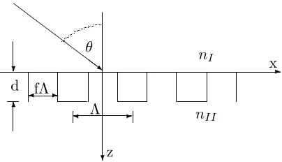
To simulate DOEs we will make use of the RCWA. The intention is to identify and calculate the reflected and transmitted waves, together they form the diffracted field. In order to do so the RCWA needs to solve the Maxwell equations, equations which govern electric and magnetic fields and waves, so also light. We’ll describe the details of the algorithm according to the paper [1]. For a sketch of the situation see figure 2.

-? Z

Z Z

Z_Z_~ ?

6

z

x

θ _n

I

nII

d

[image:6.595.73.275.188.304.2]

Λ fΛ

Figure 2: A grating in two-dimensional view. The wave comes in at an angle θ, it passes from

material I (with refractive indexnI) into material II. The height of the grating is marked by the

letter d, further there is the period Λ and the duty cycle of the ridge f.

We start with two Maxwell equations:

5 ×E= −∂B

∂t (1)

5 ×H= ∂D

∂t . (2)

Here E is the electric field, B the magnetic induction, Hthe magnetic field, defined as H=µB,

and D the electric displacement, defined as D=0E. µis the permeability of the region and 0

is the permittivity. We assume that the material in question is nonmagnetic at optical frequencies

such that µ0 = µ, with µ0 the vacuum permeability. The permittivity is written as 0, where

the relative permittivity =n2 defines the refractive index n. We are interested in the frequency

domain, i.e. we examine the behaviour of the fields for one defined frequency ω. So H is of the

general form

H(r, t) =Re[H(r) exp(jωt)] (3)

and E is

E(r, t) =Re[E(r) exp(jωt)]. (4)

When we fill those in the given Maxwell equations (1) and (2) we get

E= −j

ω 5 ×H, (5)

H= j

(7)

what we write out in components. This results in six equations. We make the assumption that

there is no variation in the y-direction, so ∂y = 0, see figure 2. One observes that the system of

six equations splits into two separate sets: One corresponding to the TE polarization, the other to TM (both for the 2-dimensional case).

2.1 TE polarization

In the TE-case we are only interested in three of the equations mentioned above, namely those

containing the y-component of the electric field (Ey):

∂Ey

∂z =jωµ0Hx, (7)

∂Hx

∂z =jω0Ey+ Hz

∂x, (8)

∂Ey

∂x =−jωµ0Hz. (9)

These three equations can be put together to form the Helmholtz equation:

52Ey+ω2µEy = 0. (10)

We specialize to a DOE with a given piecewise constant shape with period Λ (see figure 2). We

focus first on the grating region 0< z < d. In this region the relative permittivity is a piecewise

constant function ofx only. In order to get a continuous function in the grating region we expand

into a (complex) Fourier series:

(x) =

∞

X h=−∞

˜

hexp(j

2πh

Λ x), (11)

where the Fourier coefficients are ˜

0 =n2rdf +n2gr(1−f) (12)

˜

h = (n2rd−n2gr)

sin(πhf)

πh (13)

The parameters in these expressions can be found in figure 2, nrd = nII is the refractive index

of the ridge and ngr = nI the refractive index of the groove. Note that this algorithm doesn’t

work for complex refractive indices. The period spans from x=₋Λ/2 to x= Λ/2. In view of the

periodicity of the DOE, we choose the following Fourier ansatz for the electric and magnetic field for the grating region (i.e.: 0< z < d):

Egy =

∞

X i=−∞

Syi(z) exp(−jkxix), (14)

Hgx=−j r_ε

0 µ0

X i

Uxi(z) exp(−jkxix), (15)

whereSyi is the yet unknown amplitude of the wave andUxifollows from Maxwell’s equations and

is given by

k0Uxi= ∂Syi

(8)

and

kxi=k0[nIsinθ−i(λ0/Λ)] =k0nIsinθ−i

2π

Λ . (17)

with the vacuum wavenumberk0 =ω√0µ0 = 2π/λ0, where λ0 is the wavelength in vacuum. The

y-component of the electric field in the grating region is required to satisfy the Helmholtz equation (10):

52Egy+k20Egy = 0. (18)

Now the ansatz (14), (15) is inserted and we receive:

−X

i

Syikxi2 exp(−jkxix)+ X

i

∂_z2Syiexp(−jkxix)+ω2µ00 X

i X

h

Syi˜hexp(−jkx(h+i)x) = 0. (19)

From now on theiin the last term is called p:

−X

i

Syikxi2 exp(−jkxix) + X

i

∂_z2Syiexp(−jkxix) +ω2µ00 X p Syp X h ˜

hexp(−jkx(h+p)x) = 0.

(20)

We call i =h+p, but shift the indices in the former P

h: we replace i−p by i. That’s possible

becauseh extends from _−∞to +_∞:

−X

i

Syikxi2 exp(−jkxix) + X

i

∂_z2Syiexp(−jkxix) +ω2µ00 X

p X

i

Syp˜(i−_p)exp(−jk_xix) = 0. (21)

we write:

X i

(₋Syikxi2 +∂z2Syi+ω2µ00 X

p

Syp˜(i−_p)) exp(−jk_xix) = 0. (22)

what results in:

∂2Syi ∂(z0

)2 = (

kxi k0

)2Syi− X

p

˜

(i−_p)S_yp, (23)

for all i where z0

= k0z. These are called the coupled wave equations. We want to write this in

matrix form with index i, but an infinite matrix is of no numerical use. So we have to assume

convergence and choose an appropriate rangei=₋N, ..., N, withN a number which is big enough

for convergence and is yet to choose. So the size of the matrix becomes 2N + 1, starting with

i =₋N as the first entry, followed by i= ₋N + 1 until the last entryi = N. This leads to the

matrix equation

[∂2Sy/∂(z0)2] = [K2x−E][Sy]. (24)

Here Kx is a diagonal matrix with the diagonal element at positioni being equal tokxi/k0 and E

consists of the permittivity components with the entries Ei,p= ˜(i−_p).

Now we’ve got a system of second-order differential equations with a system matrix [K2_x₋E]

with constant coefficients. A solution [25] in terms of the eigenvalues of the matrix [K2_x₋E] is:

Syi(z) = n X m=1

wi,m(c+mexp(−k0qmz) +c

−

mexp[k0qm(z−d)]), (25)

Uxi(z) = n X m=1

vi,m(−c+mexp(−k0qmz) +c

−

(9)

where c+_m and c−

m are yet to define constants, wi,m is the ith component of the eigenvector related

to an eigenvalue q2

m and

vi,m =qmwi,m, (27)

where the square root of q_m2 is taken, with the positive real part.

So now the amplitudes of the fields in the grating regions are partly dealt with. But in fact we are more interested in the amplitudes of the fields in the regions I and II (see figure 2). They form

the diffracted field. We call Ri the amplitudes of the reflected waves andTi the amplitudes of the

transmitted waves. The electric fields have to fit to the fields in the grating region at the interfaces

inz= 0,z=d. Due to the given periodicity in the grating region these fields are written:

EI,y =Einc,y+ X

i

Riexp[−j(kxix−kI,ziz)], (28)

EII,y = X

i

Tiexp(−j[kxix+kII,zi(z−d)]), (29)

with the incoming wave

Einc,y= exp[−jk0nI(sinθx+ cosθz)]. (30)

When one of these fields is put back in equation (10) the relation k2 =k2_xi+k2_`,zi is revealed. We

are looking for an expression fork`,ziand therefore we get:

k`,zi=± q

k2

0n2`−kxi2 . (31)

This still leaves us with four possibilities. So, let’s first consider the case k₀2n2_` > k2_xi: That would

mean _±k`,zi is real. Filled in the transmitting field (29) we would get a wave with imaginary

exponents with an absolute value of 1 everywhere. Also with increasingzthis wave doesn’t vanish.

This is conform with the description of the far field. In order to obtain the downward direction, we

take +k`,zi. It also happens that k20n2` < k2xi for other indicesi, so that ±k`,zi is imaginary. Let’s

first consider the +-sign. Result would be a transmitted field growing in amplitude with increasing

z. As this makes no sense we look at ₋k`,zi: this time the transmitted field would approach zero.

As this is a more realistic solution we choose for this algebraic sign. All in all we get:

k`,zi=

k0[n2_`−(kxi/k0)2]1/2 k02n2` > kxi2

−jk0[(kxi/k0)2−n2_`]1/2 kxi2 > k20n2`

`=I, II. (32)

All these fields fulfill the Helmholtz equation (10). If we want to know the magnetic fields we make use of equations (7) and (9).

Now it’s time to take into account the interface conditions at z = 0 and z =d. Continuity at

the borders is required for the tangential electric field componentsEy and the magnetic field. Note

that, according to (9), continuity ofEy and Hx across the interfaces implies continuity of Hz. We

obtain four equations:

EI,y(x,0) =Egy(x,0), (33)

HI,x(x,0) =Hgx(x,0), (34)

Egy(x, d) =EII,y(x, d), (35)

(10)

and insert the fields. We multiply by exp(₋jkxlx) and integrate over x. Then orthogonality

(_Λ1 RΛ

0 exp(−jkxlx)∗exp(−jkxix)dx =δil, where δil = 1 for l =i and δil = 0 for l6= i) is used to

eliminate the dependence on x. This leads to the equations

δi0+Ri = n X m=1

wi,m[c+m+c

−

mexp(−k0qmd)], (37)

j[nIcosθδi0−(kI,zi/k0)Ri] = n X m=1

vi,m[c+m−c

−

mexp(−k0qmd)], (38)

Ti = n X m=1

wi,m[c+mexp(−k0qmd) +c

−

m], (39)

j(kII,zi/k0)Ti = n X m=1

vi,m[c+mexp(−k0qmd)−c−m]. (40)

For purposes of implementation it appears to be convenient to write these in matrix forms:

δi0 jnIcosθδi0

+

I

−jY_I

[R] =

W WX V -VX c+ c− (41) and WX W XV -V c+ c− = I jY_II

[T] (42)

with I the identity matrix, Y_` diagonal matrices with the diagonal elements (k`,zi/k0), W the

matrix with the eigenvectors, X a diagonal matrix with the diagonal elements exp(₋k0qmd) and

V=WQ, where Q contains the eigenvalues qm in its diagonal entries. It turns out [1] to be

numerically advantageous to first calculate c±

by eliminating Ri from equations (37) and (38), or

(41) respectively, and Ti from equations (39) and (40), or (42). This results in

jY_IW+V jY_IWX₋VX VX₋jY_IIWX ₋V₋jY_IIW

c+ c−

=

jnIcosθδi0+jYIδi0

0

. (43)

This linear set of equations is now solvable by Matlab. c± can be inserted in equations (41) and

(42) to receiveRi andTi. According to the algorithm we have now computed the amplitudes of the

reflected and transmitted lightwaves. When these are inserted back in the original ansatz (14) and (15) we obtain the electric diffracted fields. They illustrate where and how the light of the DOE is spreading.

The diffraction efficiency is the fraction of energy that is transported by a certain order relative to the energy of the incoming light. It is calculated for the reflected and transmitted case separately. First the Poynting vector is computed:

S= 1

2µ0

Re(E_×B∗). (44)

(11)

indexiand equation (6), this leads to

Sri=

1 2µ0ω

RiR

∗

iRe  

kxi

0

−kI,zi



 (45)

for the reflected field,

Sti = 1

2µ0ω

TiTi∗Re  

kxi

0

kII,zi 

 (46)

for the transmitted field and

Sinc=

1 2µ0ω

Re

 

k0nIsinθ

0

k0nIcosθ 

 (47)

for the incoming light. Now only the vertical contribution of the reflected and transmitted orders is considered and divided through the vertical contribution of the incoming field to obtain the ratio we are looking for. As for the reflected wave, which travels in the other direction as the incoming

and transmitted part of the field, we are taking the absolute value of Re(₋kI,zi). Therefore we

arrive at the expressions:

DEri =RiR

∗

iRe( kI,zi k0nIcosθ

) (48)

and

DEti =TiT

∗

iRe(

kII,zi k0nIcosθ

) (49)

for the diffraction efficiencies of the reflected and transmitted waves of order i. Conservation of

energy requires that the sum of these should equal 1:

X i

(DEri+ DEti) = 1. (50)

This expression can serve as a consistency check for our computations.

2.2 TM polarization

The implementation of the TM polarization isn’t very different from that of the TE case. This

time the leading field is the magnetic field Hy. Expressions are the same as in the TE case if not

otherwise stated. Again, we start with the Maxwell equations (1) and (2). When filling (3) and (4)

into (1) and (2) we get six equations. Now we pick out those which contain they-component ofH:

∂Hy

∂z =−jωEx, (51)

∂Hy

∂x =jωEz, (52)

∂Ex ∂z −

∂Ez

(12)

The fields are as follows:

HI,y = exp[−jk0nI(sinθx+ cosθz)] +

X i

Riexp[−j(kxix−kI,ziz)], (54)

HII,y = X

i

Tiexp{−j[kxix+kII,zi(z−d)]}, (55)

Hgy = X

i

Uyi(z) exp(−jkxix) (56)

and

Egx=j r

µ0 0

X i

Sxi(z) exp(−jkxix). (57)

The ansatz of the fields (54)-(57) is inserted in equations (51)-(53) and we receive (in matrix form):

[∂2Uy/∂(z

0

)2] = [EKxE

−₁

Kx−E][Uy]. (58)

We’ll need the eigenvalues of the matrix [EKxE−1Kx−E] to solve this system of second order

differential equations. The amplitudes of the magnetic and electric fields are given by:

Uyi(z) = n X m=1

wi,m(c+mexp(−k0qmz) +c

−

mexp[k0qm(z−d)]) (59)

and

Sxi(z) = n X m=1

vi,m(−c+mexp(−k0qmz) +c−mexp[k0qm(z−d)]), (60)

withwi,m and qm as defined in the TE case, butvi,mare the elements of the matrixV=E

−₁

WQ. This makes the resulting matrix equation slightly different:

jZ_IW+V jZ_IWX₋VX VX₋jZIIWX −V−jZIIW

c+ c−

=

jcosθδi0/nI+jZIδi0

0

. (61)

Here X is the same as above and Z` (` = I, II) are diagonal matrices with the diagonal entries

kI,zi/k0n2_`.

Also the diffraction efficiency of the transmitted orders changes:

DEti=TiTi∗Re( kII,zi

n2 II

)/(k0cosθ

nI

). (62)

2.3 Multilayer systems

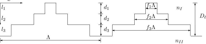
The next step was to move on to a system with several layers, as to be seen in figure 3. As before, we focus on a TE configuration first. Fourier expansions are defined separately for each

layer. The field of layer` is given by:

E`,gy = X

i

(13)

Λ

6 ?d1 6 ?d2 6 ?d3

6 ? D` l1 l2 l3 nI nII

-f1Λ

f2Λ

f3Λ

-? x

[image:13.595.93.484.45.130.2]

z

Figure 3: A surface-relief grating with three layers.

with

S`,xi(z) = n X m=1

w`,i,m(c+`,mexp(−k0q`,m(z−D`+d`) +c

−

`,mexp[k0q`,m(z−D`)]) (64)

and D` =P`p=1dp, i.e. the coordinate of the height.

For each layer we’ve got a matrixE`,W`,V` andX`. Also thec

±

` coefficients and the fields of

course, have to be calculated for each layer. The relation between the coefficients is derived from the interface conditions between the layers and results in:

W`−₁X_`−₁ W_`−₁

V`−₁X_`−₁ −V_`−₁

c+_`−₁

c−_`−₁

=

W` W`X` V` −V`X`

c+_` c−_`

, (65)

so that the transitions are continuous. And the matrix equations at the outmost boundaries become

δi0 jδi0cos(θ)nI

+

I

−jYI

[R] =

W1 W1X1 V1 -V1X1

c+₁ c−₁

(66)

and

WLXL WL

VLXL −VL c+_L c−_L

=

I jYII

[T]. (67)

Combining equations (65) till (67) leads to:

δi0 jδi0cos(θ)nI

+

I

−jY_I

[R] =

L Y `=1

W` W`X` V` −V`X`

W`X` W` V`X` −V`

−1

I jY_II

[T]. (68)

Unfortunately, this last equation isn’t stable if solved directly forRandT. The paper suggested

two methods implementing the system otherwise. The following one was used: At first the right

side of equation (68) (only with the factorL) is changed into

WL WLXL

VL −VLXL

WLXL WL

VLXL −VL −1

I jYII

[T] =

WL WLXL

VL −VLXL

XL 0

0 I

−1

WL WL

VL −VL −1

fL+1 g_L+1

[T],

(69) with fL+1 g_L+1 = I jY_II

(70)

(14)

WLXL WL

VLXL −VL −1

=

XL 0

0 I

−1

WL WL

VL −VL −1

. (71)

We now state

aL bL =

WL WL

VL −VL −1

fL+1 g_L+1

. (72)

We substitute that in (69):

WL WLXL

VL −VLXL

XL 0

0 I

−1

aL bL

[T]. (73)

Further we introduce another intermediate quantityTLthroughT=a−_L1XLTL. This is substituted

into the last expression which leads to

WL WLXL

VL −VLXL

I bLa

−₁

L XL

[TL] (74)

which we set equal to

fL g_L

[TL]. (75)

Now equation (68) becomes

δi0 jδi0cos(θ)nI

+

I

−jY_I

[R] =

L−₁

Y `=1

W` W`X` V` −V`X`

W`X` W` V`X` −V`

−1

fL g_L

[TL], (76)

i.e. the product on the right-hand side has one factor less. After repeating this analogously for all further inner layers we end up with

δi0 jδi0cos(θ)nI

+

I

−jYI

[R] =

f1 g₁

[T1], (77)

which is reformulated:

−I f1

jYI g1 R T1 = δi0 jδi0cos(θ)nI

(78)

so that Rand T1 can now be calculated directly (f1 and g1 follow from equations (74) and (75)).

Finally, Tis computed by

T=a−_L1XL...a

−₁

` X`...a

−₁

1 X1T1. (79)

Calculating the electric and magnetic fields turned out to be slightly more difficult than in the

one-layer system, since the coefficients c±_` weren’t calculated explicitly (as before).

Equation (67) is reformulated:

−WL ffL+1

−VL ggL+1

c−_L c+_L+1

=

WLXL VLXL

c+_L (80)

(15)

Now we want to determine a relation between the coefficients, let’s say c−_L =aaLc+_L. We also

assignc+_L+1 =bbLc+_L and substitute this in equation (80) what results in:

aaL bbL

=

−WL ffL+1

VL ggL+1 −1

WLXL VLXL

(81)

The general formula forff_` and gg_` is

ff` gg_`

c+_` =

W` W`X` VL −V`X`

c+_` c−_` .

(82)

Now all coefficients aa` and bb` can be calculated, starting with c+1 all other coefficients c

±

` can

be determined. c+₁ follows from the reformulated equation (66):

δi0 jδi0cos(θ)nI

+

I

−jYI

[R] =

ff1 gg₁

c+₁. (83)

The problematic inversion of equation (65) is avoided this way.

The TM polarization for the multiple layer system is very similar to the multi-layered TE

polarization. Instead of the eigenvalues of matrix [K2_x₋E`] we take those of [E`KxE

−₁

` Kx−E`] and

we useZ`instead ofY`. Furthermore, the first matrix in equation (66) will become

δi0 jδi0cos(θ)/nI

(16)

3 Benchmarking results

A program that implements the theory above has been implemented in Matlab. In order to avoid stability problems some matrix equations had to be rewritten, as was to be seen in the last section.

The input parameters are:

• TE or TM

• Wavelength in free space λ0

• Angle of incidenceθ

• Refractive indices nI and nII

• Number of layers l(in a multilayer system)

• Number of Fourier harmonicsN

• Grating period Λ

• Height of layer(s) d`

• Duty cycle f`

As output we get:

• Amplitudes of the reflected and transmitted waves Ri and Ti

• Diffraction efficiencies of ith order, reflectedDEri and transmitted DEti

• Electric and magnetic fieldsE and H

3.1 TE polarization

This code was tested by a reproduction of figure 2 from [1], the results are shown in figure 4: Left above, the two curves agree quite well, only the dips on the right side don’t reach zero like the original graph. The plot next to it on the right is also very similar to the original, the amplitude and frequency look the same. But again the curve doesn’t reach 0 at the minima, also it’s quite shaky as if there’s another frequency present. The lower left plot agrees very much with the TM curve. The last plot, right below, matches very good with the figure in the paper. Note that the lower left plots of the TE (figure 4) and TM polarization (figure 7) are exchanged in [1].

To verify the results of this program the free software ’Optiscan’ by the University of Arizona (2005), written by students, was used. It also employed the Rigorous Coupled Wave Theory but

the code was not accessible. Also it used a slightly different coordinate system, as a positive θ in

my code corresponds to a ₋θ in ’Optiscan’. The configurations in this program also couldn’t be

changed to reproduce figure 4. So two other cases with varied wavelength were chosen. The results for the transmitted and reflected diffraction efficiencies is shown in figure 5. The agreement in all cases was satisfying.

(17)

0 1 2 3 4 5 0

0.2 0.4 0.6 0.8 1

period=10*wavelength

DEt(1)+DEr(1)

d/wavelength

45 46 47 48 49 50

0 0.2 0.4 0.6 0.8 1

d/wavelength

DEt(1)+DEr(1)

0 1 2 3 4 5

0 0.2 0.4 0.6 0.8 1

d/wavelength

DEt(1)+DEr(1)

period=wavelength

45 46 47 48 49 50

0 0.2 0.4 0.6 0.8 1

d/wavelength

DEt(1)+DEr(1)

[image:17.595.104.488.198.482.2]

period=wavelength

Figure 4: Here n1 = 1, n2 = 2.04, θ= 10◦, the duty cycle equals 0.5 and the number of Fourier

harmonics is 101 (N = 50). The first-order diffraction efficiency (TE) is depicted against the ratio

d/λ0. In the graphs above Λ = 10λ0 and below Λ =λ0. On the left side the low values of the ratio

d/λ0 are depicted, on the right plots its magnitudes reach 50. This is a reproduction of figure 2 in

(18)

0.4 0.5 0.6 0.7 0.8 0.9 1 0

0.1 0.2 0.3 0.4 0.5 0.6 0.7

wavelength [µm]

Diffraction efficiency transmitted

0 order 1 order −1 order

(a)

0.4 0.5 0.6 0.7 0.8 0.9 1

0 0.01 0.02 0.03 0.04 0.05 0.06 0.07 0.08

wavelength [µm]

Diffraction efficiency reflected

0 order 1 order −1 order

(b)

0.4 0.5 0.6 0.7 0.8 0.9 1

0 0.1 0.2 0.3 0.4 0.5 0.6 0.7

wavelength [µm]

1 order −1 order 0 order

(c)

0.4 0.5 0.6 0.7 0.8 0.9 1

0 0.01 0.02 0.03 0.04 0.05 0.06 0.07 0.08

wavelength [µm]

[image:18.595.84.549.165.501.2]

(d)

Figure 5: Here n1 = 1, n2 = 2.04, height= 400nm, Λ = 1µm, the duty cycle equals 0.5 and the

number of Fourier harmonics is 101 (N = 50). The wavelength is varied. Above the transmitted

and reflected diffraction efficiency at 0 degrees is depicted. The 1st and ₋1st order are identical

in this symmetric case, as it should be. Below the transmitted and reflected diffraction efficiency for 10◦

(19)

x [µm]

z [µm]

real part of E−field (TE polarization) [V/m]

0 0.5 1 1.5 2 −0.5

0

0.5

1

[image:19.595.85.337.78.279.2]

1.5 −2 −1.5 −1 −0.5 0 0.5 1 1.5 2 2.5

Figure 6: The electric field for the grating with λ0 = 0.355µm, Λ = 1µm, n1 = 2.04, n2 = 1,

θ= 10◦

, duty cycle equals 0.5, the number of Fourier harmonics is 101 (N = 50) and height of the

layer=0.4µm. The light wave enters from above and the grating structure is also plotted.

Other benchmark tests were done with another paper [24]. Here the Finite Element Method was used to analyse binary gratings and design optimization was done by gradient descent. Respectively a two-, three-, four- and five-beam splitter was presented. We’ll look at the first two examples, in

both cases for perpendicular incidenceθ= 0◦

. The parameters are listed in table 1.

Table 1: The parameters of the two-beam splitter (a) and three-beam splitter (b) from [24].

nI nII λ0 Λ d f

a) 1.5315 1 0.633µm 2λ0 0.734µm 0.72

b) 1.5315 1 0.633µm 2λ0 0.43µm 0.58

Λ 6?d1

nI

nII

-f1Λ

-?x z

In table 2 the transmitted energy of the desired orders is compared: the first column lists the results of the cited paper, the second column tells what our RCWA program calculated.

These numbers are very similar, but it’s striking that the diffraction efficiency of the 1th_and₋₁th

order in the FEM calculation is not exactly the same, although the light comes in perpendicularly.

Symmetry therefore requires identical diffraction efficiencies for orders_±1. Experimenting with the

duty cycle revealed that these parameters didn’t reach the optimum: with f = 0.77 the numbers

[image:19.595.73.527.434.490.2]

(20)

[image:20.595.72.387.364.435.2]

Table 2: The transmitted diffraction efficiencies of the two- and three-beam splitter calculated by means of the FEM ([24]) and the RCWA.

a) b)

DEt FEM RCWA RCWA (f = 0.77) FEM RCWA

-1 order 0.435 0.4351 0.4456 0.295 0.3204

0 order 0.023 0.023 0.009 0.279 0.2469

(21)

3.2 TM polarization

The results for TM polarization were comparable to those of TE: The graphs were similar (see figure 7). Again the low marks don’t reach zero. Our program did not work for a configuration with more than five layers and a large period, due to.

0 1 2 3 4 5

0 0.2 0.4 0.6 0.8 1

d/wavelength

DEt(1)+DEr(1)

45 46 47 48 49 50

0 0.2 0.4 0.6 0.8 1

d/wavelength period=10*wavelength

DEt(1)+DEr(1)

0 1 2 3 4 5

0 0.2 0.4 0.6 0.8 1

d/wavelength period=wavelength

DEt(1)+DEr(1)

45 46 47 48 49 50

0 0.2 0.4 0.6 0.8 1

d/wavelength period=wavelength

[image:21.595.107.486.153.423.2]

DEt(1)+DEr(1)

Figure 7: Reproduction of figure 2 from [1], TM polarization. Here nI = 1, nII = 2.04, θ = 10◦,

duty cycle equals 0.5 and the number of Fourier harmonics is 101 (N = 50). The first-order

diffraction efficiency is depicted.

(22)

0.4 0.5 0.6 0.7 0.8 0.9 1 0

0.1 0.2 0.3 0.4 0.5 0.6 0.7

wavelength [µm]

(a)

0.4 0.5 0.6 0.7 0.8 0.9 1

0 0.01 0.02 0.03 0.04 0.05 0.06 0.07 0.08 0.09

wavelength [µm]

(b)

0.4 0.5 0.6 0.7 0.8 0.9 1

0 0.1 0.2 0.3 0.4 0.5 0.6 0.7

wavelength [µm]

(c)

0.4 0.5 0.6 0.7 0.8 0.9 1

0 0.01 0.02 0.03 0.04 0.05 0.06 0.07

wavelength [µm]

[image:22.595.84.547.166.511.2]

(d)

Figure 8: Here nI = 1, nII = 2.04, height= 0.4µm, Λ = 1µm, the duty cycle equals 0.5 and the

number of Fourier harmonics is 161 (N = 80). The wavelength is varied. The transmitted and

reflected diffraction efficiency at 0 degrees with TM polarization is depicted in (a) and (b). The 1st

and ₋1st _{order are identical because} _θ _{= 0}◦

. The transmitted and reflected diffraction efficiency

for incidence angle θ = 10◦

(23)

3.3 Multilayer systems

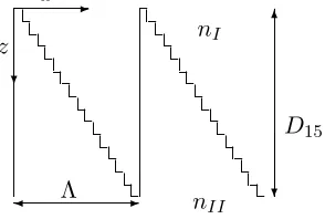
Also a multilayer system has been benchmarked. First, the pictures in [18], figure 2, were

reproduced: They treated a 15-layer system, with partly quite wide and deep grooves (Λ = 10λ0

and/or d/λ0 = 50). The grating looks like a sawtooth function decreasing from left to right. Each

layer depth is 1/15 of the whole grating depthDand the stepsize in width per layer is 1/16 of the

grating period (see figure 9). In order to do so, equation (13) has to be changed, due to the no longer symmetric setting of the groove/teeth-ratio within each period. We therefore consider the equation

(x) =

n2_II for 0< x < fΛ

n2

I for fΛ< x <Λ

(84)

and apply Fourier expansion:

˜

h=j

(n2_I₋n2_II)

2πh (1−exp(−jh2πf)). (85)

Furthermore, θ = 10◦

,nI = 1, nII =nridge = 2.04 and the groove depth is being varied. The

results are to be seen in figure 10. Forλ0 = Λ both TE and TM polarization are agreeing with the

paper. But when Λ goes up to 10λ0 the TM modulation becomes unstable, due to an ill-conditioned

system in equation (79): Also with an increasing number of Fourier harmonics (N _→ 501) the curve

consists of an uncountable number of peaks, partly reaching 15. This is obviously due to the fact

that for a big period (Λ = 10λ0) and in general the TM polarization more harmonics are needed.

In the TE case it’s still good coinciding with the paper.

-? x

z

Λ

-6

? D15 nI

[image:23.595.94.241.379.478.2]

nII

Figure 9: A sawtooth grating withD15= 1.5Λ.

Again, ’Optiscan’ was used to compare the curves, see figure 11. We observed virtually no differences versus our results.

With the present solver for multilayer systems it’s also possible now to simulate a structure of finite thickness (see figure 12).

In this case nI =nII. For a simple example, a binary grating with finite thickness, we make

(24)

0 1 2 3 4 5 0

0.2 0.4 0.6 0.8 1

d/wavelength

DEt(1)+DEr(1)

0 1 2 3 4 5

0 0.2 0.4 0.6 0.8 1

d/wavelength

DEt(1)+DEr(1)

period=wavelength

45 46 47 48 49 50

0 0.2 0.4 0.6 0.8 1

d/wavelength

DEt(1)+DEr(1)

45 46 47 48 49 50

0 0.2 0.4 0.6 0.8 1

period=wavelength

d/wavelength

[image:24.595.100.488.182.491.2]

DEt(1)+DEr(1)

Figure 10: Reproduction of graph from [18], figure 3. The red dashed line represents the TE results and TM comes along with the blue curves. It depicts the first order diffraction efficiency dependence

with nII = 2.04, nI = 1 at θ = 10◦, the grating consists of a 15 layer system. The two pictures

above use Λ = 10λ0, as this is a large system, only the TE polarization produced stable results. In

the plots below Λ =λ0 holds, here also the TM curves are steady. The matching between the plots

(25)

0.4 0.5 0.6 0.7 0.8 0.9 1 0

0.1 0.2 0.3 0.4 0.5 0.6 0.7

wavelength [µm]

(a)

0.4 0.5 0.6 0.7 0.8 0.9 1

0 0.01 0.02 0.03 0.04 0.05 0.06

wavelength [µm]

(b)

0.4 0.5 0.6 0.7 0.8 0.9 1

0 0.1 0.2 0.3 0.4 0.5 0.6 0.7

wavelength [µm]

(c)

0.4 0.5 0.6 0.7 0.8 0.9 1

0 0.01 0.02 0.03 0.04 0.05 0.06 0.07

wavelength [µm]

[image:25.595.82.550.169.510.2]

(d)

Figure 11: Here for the TE polarization (a,b) the wavelength is varied from 0.4µm to 1µm in a

two-layer system. We use θ = 10◦

, the period is 1µm, N = 41 and the height of one layer is

0.2µm. The duty cycles are 0.3 and 0.6 respectively. Here the transmitted and reflected diffraction

efficiencies of the ₋1st _{(green), 0}th _{(blue) and 1}st _{order (red) are depicted. In the lower pictures}

(c) and (d), the wavelength for the TM polarization is varied from 0.4 µmto 1 µm,θ= 10◦

(26)

-?

x

z nI

nrd

[image:26.595.78.554.224.545.2]

nII

Figure 12: A grating of finite thickness.

0.4 0.5 0.6 0.7 0.8 0.9 1

0 0.1 0.2 0.3 0.4 0.5 0.6 0.7 0.8 0.9

wavelength [µm]

(a)

0.4 0.5 0.6 0.7 0.8 0.9 1

0 0.1 0.2 0.3 0.4 0.5 0.6 0.7 0.8 0.9

wavelength [µm]

(b)

0.4 0.401 0.402 0.403 0.404 0.405

0 0.1 0.2 0.3 0.4 0.5 0.6 0.7

wavelength [µm]

(c)

0.4 0.401 0.402 0.403 0.404 0.405

0 0.05 0.1 0.15 0.2 0.25 0.3 0.35 0.4 0.45

wavelength [µm]

(d)

Figure 13: The transmitted (a) and reflected (b) diffraction efficiencies of three orders with a multi

layer system with finite thickness: height (of each layer) =0.4µm, nI =nII = 1 and nrd = 2.04.

The grating period is 0.5. Here Λ = 0.1µm and θ = ₋10◦

. The result agreed with that from

’Optiscan’. The transmitted diffraction efficiencies of the ₋1st (green), 0th (blue) and 1st order

(red) are depicted. In (c) and (d) the transmitted and reflected diffraction efficiency of the ₋1st_,

0thand 1storder with another grating of finite thickness: Λ = 1µm,θ=₋10◦

, height of the grating

(27)

4 Design of a three-beam splitter

Now the RCWA solver is to be used to design a three-beam splitter. Therefore we will look for

the appropiate choice of parameters. Some will be variable, others stay fixed. A number ofN = 50

Fourier harmonics appeared to be sufficient for all simulations carried out during optimization. Some first considerations concern the period Λ, as to be seen in the following section.

4.1 Determination of the number of orders

In order to design a three-beam splitter, we have to ask: How can we predict the number of orders a grating transmits? The following rough reasoning shows why that depends on the

wavelength λ0 and the period Λ. We start with Huygens principle when looking at the grating:

Here light waves in the slits at z= 0 behave like point sources interfering with each other. In the

directions where constructive interference takes place, a diffractive order is observed. The order 0 always exists as it relates to those waves from the point sources that go straight downwards. Elementary waves from all equivalent points meet in-phase (figure 14(a)) with the parallel wave from the point source one period further. Hence, these light waves interfere constructively.

But there are also other directions where this happens. The waves propagating under the respective angle are superimposed with the same phase with waves from the equivalent point sources, i.e. the waves are interfering constructively (see figure (14(b)). This occurs when the

distance`is a multiple of the wavelengthλ, the distance between two wavefronts with equal phase.

λis the wavelength in the material withλ= λ0

nI I. That means

`=mλ (86)

withm an integer which indicates the diffraction order. According to the picture one has

sinα = `

Λ. (87)

Both expressions lead to the grating equation

Λ sinα=mλ0

nII

. (88)

This equation may be read as follows: For given wavelength and period, the diffractive order m

appears under an angleα.

We also can consider the situation with light coming in under an angle (figure 14(c)). The

picture looks similar, but we deal now with two distances we have to take into account: `1 and

`2. Incoming waves that pass through adjacent equivalent points differ by l1 and l2 in optical

path length. When now l1kI+l2kII =m2π the wavefronts will meet again in phase and interfere

constructively. We therefore get the equation

Λ(nIIsinα+nIsinθ) =mλ0. (89)

Now we want to know which values of Λ are allowed, i.e. for which range of periods Λ the

grating supports only the fundamental and first diffraction orders (hereθ= 0◦

(28)

-?

x

z

? ?

Λ

-(a)

@@ @@ @@ @@ @@ @@ @@

@@

? ?

-@ @ α

` Λ

λ

(b)

nI

nII _@_@@@

@@ @@ @@ @@ @@

@@

A_A AAU A

A AAU

-θ `1KAAU

@ @ α

`2

Λ

λ

[image:28.595.95.464.62.195.2]

(c)

Figure 14: Interference of wavefronts from two equivalent point sources in the periodic grating. (a): the diffractive order 0 and (b) order 2. The wavefronts are interfering constructively. (c) shows

interference of wavefronts in a grating with incoming light from above under the angleθ.

to remember thatα mustn’t reach 90◦

, otherwise the situation wouldn’t make sense any more. So, according to equation (88) the grating supports a diffraction order of 1 and no second order, if

2λ0

nII ≥

Λ> λ0 nII

. (90)

Also the transmitted electric field according to the RCWA formulation can be used to find out

this condition. We consider the equation for the transmitted field (29) and look at kII,zi (equation

(32)) for the electromagnetic far field. The corresponding inequation and equation (17) withθ= 0◦

lead to the condition:

Λ> mλ0 nII

. (91)

(29)

4.2 Optimization

The task is now to design a DOE, here a grating that, if illuminated by laser light, transmits only three orders, each containing approximately the same energy. In practice this is the easiest

to realise if one concentrates on the orders -1, 0 and 1. As we set θ= 0◦

the diffraction efficiency of the orders 1 and -1 are equal. But still the other variables have to be optimized to distribute

1/3 of the transmitted diffraction efficiencies on each of the three orders. This can be expressed by

requiring the quantity

Err = (DEt−₁−

1 3)

2_{+ (DE}

t0−

1 3)

2_{+ (DE}

t1−

1 3)

2 ₍₉₂₎

to become as small as possible. For every order the difference between the real transmitted energy

and the requested one third is calculated, the results are squared and added 1. Some parameters

can be fixed already in advance:

• TE polarization

• incidence angle θ= 0◦

• wavelengthλ0 = 0.6328µm (red laser)

• refractive indicesnI = 2.04 and nII = 1 (air)

The varied parameters are:

• height d` of layer `

• number of layers

• duty cycle f` of layer `

Optimization is realized by first determining the number of layers. For only one layer we

therefore are dealing with two parameters, d1 and f1. As for the period, 1.1λ,1.25λ,1.5λ,1.75λ

and 2λ were tried out. We took a stepsize of 0.01 and then calculated Err for all the possible

gratings of d1 within 0→ 1µm and f1 between 0 and 1. After that, the system with the smallest

Err was picked. With a two-layer system,f2 is added but we keepd2 =d1, as optimizing with more

than three variables results in a computing time of weeks. Also here the possible combinations are calculated and searched for the best values. For practical reasons, the duty cycle of the upper layer had to be smaller than the duty cycle of the lower layer. Due to the direct search method, adding a third layer resulted in a computing time of weeks, as it considers four variables. For this reason a four-layer system was not considered.

First, a one-layer system was optimized. The results are to be seen in table 3a). Following

equation (88), the period of Λ = 1.25λ results in an outcoming angle α = _±53.13◦

of the first modes. It is striking that the teeth of the grating are very narrow. The absolute electric field with a sketch of the grating is depicted in figure 16(a). The landscape (i.e. the function Err) is depicted

1

More generally: the desired value of distribution is subtracted from the diffraction efficiency of the respective order and squared according to the Least Squares method. It is also possible to add a weighting factor to a certain

term. For example: a small Err0_{= (DE}

t₋1₋0_.5) 2

+ 3(DEt0) 2

+ (DEt1₋0_.5) 2

(30)

[image:30.595.67.526.84.260.2]

Table 3: The optimized gratings and the resulting Err.

Λ d1 d2 d3 f1 f2 f3 DEt±₁ DE_t0 Err

a) 1.25λ 0.89µm 0.92 31.49% 30.68% 0.0014

b) 1.25λ 0.67µm 0.67µm 0.62 0.95 32.64% 32.48% 0.00016897

c) 1.25λ 0.67µm 0.62 1.11% 86.13% 0.4865

d) 1.25λ 0.67µm 0.68µm 0.62 0.95 32.82% 32.59% 0.0001088

e) 1.25λ 0.8µm 0.8µm 0.58 0.79 29.86% 29.55% 0.0039

f) 1.75λ 0.38µm 0.38µm 0.38µm 0.66 0.7 0.74 30.52% 29.94% 0.0027

Λ 6?d1

nI

nII

-f1Λ

-?x z

Λ 6

?d1 6

?d2 6?D` nI

nII

-f1Λ f2Λ

-?x

z _Λ _-6

?d1 6 ?d2 6 ?d3

6 ?D` nI

nII

-f1Λ

f2Λ f3Λ

-? x z

in figure 15(a). There exist several dips, but the smallest errors are still to be found in the area of the big duty cycles.

When we are switching to a two-layer system, we are keeping the same height for both layers and are therefore dealing with three variables. So we get for every value of the first duty cyle an error landscape as in figure 15(a), but only the configurations where the upper duty cycle is smaller than the lower one are considered. Adding this second layer delivered a better result, see table 3b). The corresponding field is to be seen in figure 16(b). Also, here the teeth of the lower

layer are very narrow. The error landscape for f1= 0.62 is to be seen in figure 15(b). To estimate

the influence of the lower layer a similar system with the same values but with only the first layer was considered (table 3c)). Surprisingly, this changed the distribution of the diffraction efficiencies enormously: For the corresponding electric field, see figure 16(c). Apparently, the rods have a significant influence on this grating. This is quite surprising, given their narrow appearance. Now, both duty cycles and only the height of the upper layer were fixed and optimization (over the height of the lower layer) delivered the grating with the specification of table 3d), a slightly better system with even a bit longer lower teeth. The electric field of this grating is displayed in figure 17(a).

Also varying over both heights (still with fixed duty cycles) revealed the same data. So this system was considered to be the best for this project. If one looks for a grating with more robust

appearance one should fix a maximum range for the lower layer (0.8). For Λ = 1.25λand the same

height for both layers this was tested and resulted in the system in table 3e). The result however is slightly worse than configuration (d), for the field see 17(b).

Adding a third layer didn’t give better results. For the parameters, see table 3f). The outcoming

angle α amounts to 34.85◦

. The field is to be seen in figure 17(c). At a first glance the regular

slope (0.38/0.04) of the duty cycles suggested that a certain form of the teeth could also influence

(31)

X: 0.89 Y: 0.92 Index: 0.001382 RGB: 0, 0, 0.563

height [µm]

duty cycle

0 0.2 0.4 0.6 0.8 1

0 0.1 0.2 0.3 0.4 0.5 0.6 0.7 0.8 0.9 1 0.05 0.1 0.15 0.2 0.25 0.3 0.35 0.4 0.45 0.5 (a)

X: 0.67 Y: 0.95 Index: 0.000169 RGB: 0, 0, 0.563

height [µm]

lower duty cycle

upper duty cycle = 0.62

0 0.2 0.4 0.6 0.8 1

[image:31.595.88.522.94.246.2]

0.65 0.7 0.75 0.8 0.85 0.9 0.95 1 0.05 0.1 0.15 0.2 0.25 0.3 0.35 0.4 0.45 0.5 0.55 (b)

Figure 15: The function Err of a one-layer grating (a) and of a two-layer grating (b), the latter for

one specified value of f1 = 0.62.

x [µm]

z [µm]

0 0.5 1 1.5 −1 0 1 2 3 4 5 6 7 8 9 0.5 1 1.5 2 2.5 3 3.5 4

(a) x [µm]

z [µm]

0 0.5 1 1.5 −1 0 1 2 3 4 5 6 7 8 0.5 1 1.5 2 2.5 3 3.5 4

(b) x [µm]

z [µm]

[image:31.595.85.542.328.436.2]

0 0.5 1 1.5 −1 0 1 2 3 4 5 6 7 0.5 1 1.5 2 2.5 3 3.5 4 (c)

Figure 16: The (absolute) electric fields of the one-layer grating (a), the two-layer grating (b) and the latter without the lower layer (c).

x [µm]

z [µm]

0 0.5 1 1.5 −1 0 1 2 3 4 5 6 7 8 0.5 1 1.5 2 2.5 3 3.5 4

(a) x [µm]

z [µm]

0 0.5 1 1.5 −1 0 1 2 3 4 5 6 7 8 9 0.5 1 1.5 2 2.5 3 3.5 4

(b) x [µm]

z [µm]

0 0.5 1 1.5 2 0 1 2 3 4 5 6 7 8 0.5 1 1.5 2 2.5 3 3.5 4 (c)

[image:31.595.77.545.516.625.2]

(32)

Also, the gradient descent method was tried out to find a minimum of Err. The heights d`

and duty cycles f` for three layers were varied, their gradients were calculated to look for the

smallest values of Err. But as it seemed the error landscape was so full of local minima, that using this program didn’t deliver any feasible results. On the other hand it has been used to verify the optimized gratings already found.

So concludingly, some tests with slightly varying data were performed on grating d). We were mainly interested in the stability of certain parameters: in figure 18 the duty cycle and height of the second layer, the period and the angle of incidence was diversified. This way it was verified that Err at the specified point really reaches a minimum. The graphs also tell about the range in which the parameters can be changed without significant effect on the outcome, i.e. the graphs could provide a basis for an analysis of fabrication tolerances. The lower duty cycle is, as it seems, the most sensitive parameter. Varying the period/wavelength-ratio, on the other hand, has little effect.

We also simulated the same grating for a TM-polarized wave. This resulted in a much worse

performance with DEt±₁ = 4.9% and DE_t0 = 80.53%, Err = 0.3845. A three-beam splitter

(33)

0 0.5 1 0

0.2 0.4 0.6 0.8

DE transmitted

0.7 0.8 0.9 1 0

0.2 0.4 0.6 0.8

0.4 0.6 0.8

0 0.2 0.4 0.6 0.8

0 0.5 1

0 0.2 0.4

Duty cycle upper layer

Err

0.7 0.8 0.9 1 0

0.2 0.4

Duty cycle lower layer

0.4 0.6 0.8

0 0.2 0.4

wavelength [µm] 0 order 1/−1 order

0 0.5 1

0 0.2 0.4 0.6 0.8

DE transmitted

0 0.5 1

0 0.2 0.4 0.6 0.8

1.150 1.2 1.25 1.3

0.2 0.4 0.6 0.8

0 0.5 1

0 0.1 0.2 0.3 0.4

height upper layer [µm]

Err

0 0.5 1

0 0.1 0.2 0.3 0.4

height lower layer [µm]

1.150 1.2 1.25 1.3

0.1 0.2 0.3 0.4

[image:33.595.98.453.119.614.2]

period/wavelength 0 order 1/−1 order

(34)

5 Conclusion

The Rigorous Coupled Wave Analysis has been implemented according to the formulation in [1]. Both TE and TM polarization were considered. First, gratings consisting of one layer were examined. Those gratings are periodic in one dimension, while the angle of incidence can also be varied in one dimension. The algorithm calculates the amplitudes of the reflected and transmitted waves. Those can be used to determine the diffraction efficiencies and the electric and magnetic fields. The same is possible for gratings with several layers. The computational effort grows with every added layer since the number of unknowns and matrix inversions increases. The 15 layer system referred to in figure 10 in the TM case with a big period didn’t show stable results at all. Five layers needed more Fourier harmonics but could be calculated. Also finite gratings can be analysed.

In principle, although tested so far only for lossless dielectric structures, the technique should work for metallic structures as well, provided that no additional numerical difficulties occur [16], [17]. Note that if we are dealing with a metallic grating, part of the energy is absorbed by the material and therefore (50) wouldn’t hold anymore. Also, here a grating of finite thickness should be considered for practical reasons.

By means of this method we designed a two-layer system that divides the energy of a straight incoming laser beam quite homogeneously into three laser rays. It is striking that the second layer is reduced to series of narrow spikes and therefore the system will probably be difficult to produce. Removing the rods or, at least trying to shorten them, resulted in a much worse performance. The same problem is encountered in the one-layer system, it performed best with a very big duty cycle. Results in a constricted, more realistic range were slightly worse. The three-layer grating might be a more practical solution: with rather broad rods it performs worse than the two-layer system but better than the restricted two-layer system.

It surely depends on the application in particular what maximum deviation from the ideal performance is acceptable. This thesis concentrated more on the theory, as these constrained optimizations weren’t carried further.

Also including more variables during optimization is an opportunity, such as the period Λ, different heights and more layers. A much more efficient numerical way to optimize would be required. Unfortunately, a straight forward gradient descent method didn’t work, as the error landscape seems to be very bumpy and the program got stuck very fast in one of the many local minima. More layers will complicate the structure for producibility, too. Another fast approach would be the direct search method with several increments: we start searching with a rough stepsize, then focus on the area with the lowest Err and search there with a smaller stepsize. This can be repeated as often as necessary.

It would be interesting to know if the parameters of e.g. a two- or four-beam splitter require similar duty cycles and parameters. Possibly these systems wouldn’t need such narrow blocks and the producibility wouldn’t be a problem at all.

(35)

References

[1] M.G. Moharam, E.B. Grann, D.A. Pommet and T.K. Gaylord. Formulation for stable and efficent implementation of the rigorous coupled-wave analysis of binary gratings. J. Opt. Soc. Am A, 12(5): 1068-1076, May 1995.

[2] http://en.wikipedia.org/wiki/Finite-difference time-domain method

[3] M. G. Moharam and T. K. Gaylord. Rigorous coupled-wave analysis of planar-grating diffrac-tion, J. Opt. Soc. Am. 71: 811-818 (1981).

[4] N. Y. Chang and C. J. Kuo. Algorithm based on rigorous coupled-wave analysis for diffractive optical elements design. J. Opt. Soc.Am. A, 18(10): 2491-2501, October 2001.

[5] Wilson, Raymond G.. Fourier series and optical transform techniques in contemporary optics : an introduction / John Wiley / 1995.

[6] K. Byun, S. Kim, D. Kim. Design study of highly sensitive nanowire-enhanced surface plasmon resonance biosensors using rigorous coupled wave analysis. OPTICS EXPRESS, 13(10): 3737– 3742, 16 May 2005.

[7] E. N. Glytsis and T. K. Gaylord. Rigorous three-dimensional coupled-wave diffraction analysis of single and cascaded anisotropic gratings. J. Opt. Soc. Am. A, 4(11): 2061–2080, November 1987.

[8] Dustin W. Carr, J. P. Sullivan, and T. A. Friedmann. Laterally deformable nanomechani-cal zeroth-order gratings: anomalous diffraction studied by rigorous coupled-wave analysis. OPTICS LETTERS, 28(18): 1636–1638, September 15, 2003.

[9] M. G. Moharam and T. K. Gaylord. Rigorous coupled-wave analysis of grating diffraction-E-mode polarization and losses. J. Opt. Soc. Am, 73(4): 451–455, April 1983.

[10] J. M. Jarem. RIGOROUS COUPLED WAVE ANALYSIS OF RADIALLY AND

AZIMUTHALLY-INHOMOGENEOUS, ELLIPTICAL, CYLINDRICAL SYSTEMS.

Progress In Electromagnetics Research, PIER 34: 89–115, 2001.

[11] J. M. Jarem. RIGOROUS COUPLED WAVE ANALYSIS OF BIPOLAR CYLINDRICAL SYSTEMS: SCATTERING FROM INHOMOGENEOUS DIELECTRIC MATERIAL, EC-CENTRIC, COMPOSITE CIRCULAR CYLINDERS. PIER 43: 181-237, 2003.

[12] Z. Zylberberg and E. Marorn. Rigorous coupled-wave analysis of pure reflection gratings. J. Opt. Soc. Am, 73 (3): 392–398, March 1983.

[13] N. Kamiya. Rigorous coupled-wave analysis for practical planar dielectric gratings: 1. Thickness-changed holograms and some characteristics of diffraction efficiency. APPLIED OPTICS, 37(25): 5843–5853, 1 September 1998.

(36)

[15] J.Jarem. A Rigorous Coupled-Wave Analysis and Crossed-Diffraction Grating Analysis of Radiation and Scattering from Three-Dimensional Inhomogeneous Objects. IEEE TRANS-ACTIONS ON ANTENNAS AND PROPAGATION, 46(5): 740–741, MAY 1998.

[16] L. Li and C. W Haggans. Convergence of the coupled-wave method for metallic lamellar diffraction gratings. J. Opt. Soc. Am. A, 10(6): 1184–1189, June 1993.

[17] G. Granet and B. Guizal. Efficient implementation of the coupled-wave method for metallic lamellar gratings in TM polarization. J. Opt. Soc. Am. A, 13(5): 1019–1023, May 1996.

[18] M.G. Moharam, D.A. Pommet, E.B. Grann and T.K. Gaylord. Stable implementation of the rigorous coupled-wave analysis for surface-relief gratings: enhanced transmittance matrix approach. J. Opt. Soc. Am A, 12(5): 1077-1086, May 1995.

[19] S. Sinzinger, J. Jahns. Microoptics. 2nd _{edition. 2003 WILEY-VCH GmbH & Co. KGaA,}

Weinheim.

[20] N. Chateau and J.-P. Hugonin. Algorithm for the rigorous coupled-wave analysis of grating diffraction. J. Opt. Soc. Am. A, 11(4): 1321-1331, April 1994.

[21] Goodman, Joseph W.. Introduction to Fourier optics / 2nd ed / McGraw- Hill / 1996.

[22] Okan K. Ersoy. Diffraction, Fourier Optics and Imaging. John Willey & Sons, Inc., 2007.

[23] S. Peng and G. M. Morris. Efficient implementation of rigorous coupled wave analysis for surface-relief gratings. J. Opt. Soc. Am A, 12(5): 1087-1096, May 1995.

[24] J. Elschner, G. Schmidt. A rigorous numerical method for the optimal design of binary grat-ings. WIAS Berlin, 1991.