Modelling the discharge of the Cidanau River in West Java with the HBV model

(1)

Modelling the discharge of

the Cidanau River in West

Java with the HBV model

(2)

Modelling the discharge of the Cidanau

River in West Java with the HBV model

Oktober 2009

Ferdinand van den Brink

(3)

Summary

Water quantity problems in rivers such as droughts and floods occur quite intermittently in Indonesia, in particular on Java, and cause economical, human and environmental problems. These problems are difficult to solve, due to the lack of knowledge. The Cidanau River, situated on Java, Indonesia, is important for the economical development of the region, because it is the only river in its surrounding (Banten province) with an adequate discharge to make the water economical exploitable using a small dam. The prediction of the discharge with the HBV model may help to make this water exploitation efficient. Furthermore it is helpful to use this model as a benchmark model for the development of a more physically based model, which will quantify the groundwater level besides the discharge. Therefore the objective of this research is to predict the discharge of the Cidanau River with the HBV model to obtain a benchmark model so that outcomes of the in the future developed physically-based model can be compared.

In this research a simplified version of the HBV model has been used. For this conceptual hydrological model nine years of daily data about rainfall and evapotranspiration are used as input for the model. Furthermore, seven calibration parameters need to be calibrated with discharge data over the same period. The result is a sound prediction of the discharge. During extreme discharges the errors are relatively high. For the low water periods errors are caused by a constant base flow. On the other hand, the spatially averaged rainfall may not properly represent the rainfall in the area during high rainfall events, causing an underestimation of the high discharge peeks.

(4)

Preface

The following report is the result of the research I did for my bachelor thesis as a part of my study Civil Engineering. During three months I have been given the opportunity to do this research at Labmath-Indonesia. Therefore I am very grateful to both directors ibu Andonowati and Brennie van Groesen, not only for the internship itself, but also for this exceptional good and unique experience in an unknown foreign country.

I also would like to thank my supervisor at Labmath, Dr. Saptomo, for his advise and for arranging diverse trips and meetings that all contributed to this report. Furthermore I would like to thank my supervisor in the Netherlands, Martijn Booij, for his helpful critics on my proceedings for the preparation and writing my final report.

Finally I would like to thank all the students working at Labmath that helped me so much to get familiar with the Indonesian culture. You were always so willing to show me so many places to which I had not been going without this help.

Thank you all.

(5)

1. Introduction

1.1 background

Indonesia faces various severe environmental problems, which are usually difficult to solve because of the lack of knowledge or measurements. Problems are, depending on the season, floods and drought causing human, industrial, agricultural and environmental harm. Java is an island with a very high pressure on the environmental resources due to its high population density and is therefore sensitive for water quantity problems. Climate changes will probably contribute a worsening of the situation. Precipitation in Indonesia is expected to increase about 6-7% (Cruz et al. 2007) on average and will have more extreme values. For example Setiawan et al. (2009) confirms this for the study area of this research, the Cidanau River. In the case of the Cidanau River it is very useful to investigate the water quantity, because it is the only river in Banten province (west Java) that has enough discharge to make water extraction economically exploitable, which makes the surrounding industry depending on this river.

Other contributions to a worsening of the hydrological situation on Java are changes in land-use, deforestation, industrialization, and changes in crop type, which usually lead to a faster run-off and might result in more flooding of rivers. The precise consequences of these changes are still unknown. From the knowledge that different type of crops does not require the same amount of water, it might be obvious that different land use exerts influence on groundwater level and water run off, although evidence is missing. To investigate these issues a hydrological model will be needed which takes properties of the region like for example its soil into account.

In general a characterization in hydrological models can be made by making a distinction in what extent the model is statistically or physically based and with regard to the spatial accuracy of data, in what extent the model is lumped or distributed (Carpenter and Georgakakos, 2006; Strezepek and Yates, 1997). The required model can be characterised as a distributed differential model (Todini, 1988), because it is discretized in time and space. This model is meant to have physically based parameters, which makes lengthy hydrological records for its calibration unnecessary. The only example of this type of models has been developed by the Danish Hydraulic institute, the British Institute of Hydrology and SOGREAH (France) and is called SHE (Abbott et al., 1986). Unfortunately, because of its complexity and high data demands it is not practical in Indonesia.

(7)

The model used is a simplified version of the HBV model. The HBV model is a widely used model, which has already been applied in at least 30 countries, as Bergström (1995) and Lindström et al. (1997) state. In Indonesia the model has not been applied as far as known. It has a sound physical description but is not so complex it has a very high data demand and does not have a lot of free model parameters, especially when a simplification is used (Lidén and Harlin, 2000).

1.2 Objective and research questions

The aim of this research is to predict the discharge with the more conventional conceptual HBV model of the Cidanau River and to obtain a benchmark model so that outcomes of the in the future developed physically-based model can be compared.

This objective can be divided in the following research questions, which will be discussed further in this report:

• What are the characteristics of the examined watershed?

• How have the used data been calculated or measured?

• What is the best way to obtain spatially averaged rainfall from the given data?

• What are sources of inaccuracy in the used data and in the results?

• Does an application of the HBV model give a good prediction for the discharge of the Cidanau River?

1.3 Outline

(8)

2. Method

2.1 The HBV model

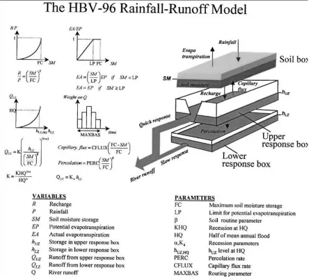
More than 35 years ago the HBV model has been developed at the Swedish Meteorological and Hydrological Institute to predict and simulate rainfall-runoff behaviour (Bergström and Forsman, 1973). Since that time it became a standard tool for runoff simulations in the Nordic countries and during the years the model faced a lot of modifications and the scope of application has also increased steadily. The HBV model can be classified as a semi-distributed conceptual rainfall runoff model and is based on a sound physical basis (Lindström et al., 1997). As its developers state, the model is meant to be understandable for users and the number of free parameters should be kept to a minimum in order to prevent over parameterization.

[image:8.595.73.520.344.743.2]

The model has six routines, namely a precipitation routine for snowfall and melting, a routine for soil moisture, a fast response routine, a slow response routine, a transformation routine and a river routing routine. For each routine relatively simple relation(s) needs to be calibrated

(9)

in order to get a good result. In the model version of Lindström et al., (1997) precipitation as function of land height and the storage of water as snow are taken into account, but for this application a simplification is used as Lidén and Harlin (2000) did. Because of the climate, snow is not relevant for Indonesia and because of the lack of data effects of height on precipitation are not taken into account. Due to this simplification only daily information about precipitation (P) and the potential evapotranspiration (EP) is needed as input for this model and the unknown parameter values are found by calibration against observed runoff. Usually at least 5 to 10 years data are needed in order that the records include a variety of hydrological events and that the effect of all subroutines of the model can be discerned (Bergström, 1995; Lindström et al. 1997; Graham and Bergström, 2001). Unfortunately, the catchment of the Cidanau River can not be divided into different subcatchments, because of the lack of suitable data in this catchment, so this application can be characterized as lumped. The used version of the HBV-96 model is shown in figure 2.1. As implied in this model scheme the water that will come into the ground is in the model regarded as the precipitation minus the actual evapotranspiration (EA), so this amount of water is added to the soil moisture storage (SM). This soil moisture storage will recharge part of its volume each time step to the upper and the lower response box and fill these boxes with water until a certain height (hUZ

and hLZ respectively). The actual evapotranspiration depends on the availability of water in the

ground, determined by LP and SM, and the potential evapotranspiration (EP). The recharge R to the groundwater is calculated with a non-linear relationship between the precipitation and the soil moisture. The upper response box dominates the runoff shortly after a rainfall event

QUZ, while the lower response box will give a long term base flow QLZ. The sum of these

outflows is the predicted outflow of the river Qcom.

2.2 Calibration and Validation

With a part of the available data from river discharges, a number of calibration parameters of the model have been optimized. The commonly used R2 (Nash and Sutcliffe, 1970), defined in formula 2.1, can be used for both making the result comparable with other applications of the HBV model, for example with Lindström et al. (1997) and for a good indication of the appropriateness of the model.

( )

2 2 1 2 1 1 n com rec i n rec rec i

Q i Q i

R

Q i Q i

= =  ₋    = −  ₋   

∑

(2. 1)

Where Qcom and Qrec are the computed and recorded discharge respectively on time step i

which goes from 1 till n.

R2 should be as close as possible to 1 in order to get the best predictions in the future. To test the performance of the model in simulating the overall water balance, the Relative Volume Error RVE can be used (Booij, 2005):

( )

1 1 100 n com rec i n rec i

Q i Q i

RVE Q i = = − =

∑

(2. 2)

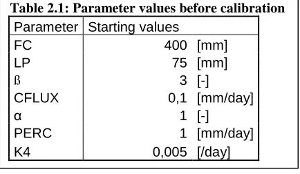
(10)

the starting values as mentioned in Lidén and Harlin (2000), see table 2.1. Each parameter is optimised individually, keeping the other parameters constant. After calibrating all parameters ones beginning with FC, all parameters had to be adjusted again, because of linear independency, till the optimal values have been reached. This process is executed for two different methods of determining the spatially averaged rainfall. Lidén and Harlin (2000) used for their automatic calibration a lower and upper limit for the parameter values as can be seen from table 2.1. During the calibration the values for the Cidanau River some parameters converged to values that exceed this suggested values. This is discussed further in chapter 5.

2.3 Determination of rainfall

For the determination of the spatially averaged amount of rainfall two methods have been used, which will be compared in chapter 4. For both methods the model has been calibrated and validated. The first method is taking an average over all the stations in the surrounding region:

( )

1 m k k P i P m =

=

∑

(2. 3)

Where P is the rainfall of station k on time step i, m is the number of stations and P is the _k

precipitation that is ought to be representative in the whole catchment.

Because some of the station are located outside the catchment and these stations will give a less representative amount of rain for the area, a second method is used, which is called the Thiessen Method. In this method the amount of rainfall from the closest station to a certain point in the catchment is ought as representative for that area (Dirks et al., 1998), defined as:

( )

1 1 1 m

k k m

k k k m k k k

A P i

P C P i

A = = = ⋅ =

∑

=

∑

⋅

∑

(2. 4)

Where A is the area of the part of the catchment that is ought to have same rainfall as in k

station k.

C

_k is a coefficient determined by

1 k k m k k A C A = =

∑

standing for the importance of a [image:10.595.72.289.200.326.2]

certain station in the Thiessen calculation.

Table 2.1: Parameter values before calibration

Parameter Starting values

FC 400 [mm]

LP 75 [mm]

ß 3 [-]

CFLUX 0,1 [mm/day]

α 1 [-]

PERC 1 [mm/day]

(11)

2.4 Evapotranspiration

The potential evapotranspiration data has already been determined for this research. This is done with the Hargreaves method, because this method requires in comparison with the more common Penman Monteith method (Monteith, 1988) less data. The Hargreaves method needs only two climatic parameters: the temperature and incident radiation, instead of the five climatic parameters required for the Penman Monteith equation: temperature, relative humidity, wind and net radiation (Wu, 1997). Requiring these data in a developing country is rather difficult, which makes the Hargreaves method more obvious (Khoob, 2008). Hargreaves method is based on the following formula:

(

)

0

10 0, 0135 17, 78

595,5 0,55

s

ET T R

T

 

= + _ _

−

  (2. 5)

Where in ET is the required potential evapotranspiration in mm, T the temperature in °C 0

and Rs the incident solar radiation in Langleys per day. One Langley is equal to one calorie

per square centimetre. Rs is the shortwave radiation that reaches the surface on a certain

place, which will be less than the radiation send by the sun Ra, because of interception from

particles and clouds in the atmosphere. Because weather data is unavailable, Ra is assumed as

equal to the incoming radiation at a cloudless day and multiplied with a constant factor to represent clouds. R_a has been calculated according to FAO guidelines (Allen et al. 1998) as described in formula 2.6:

( )

24 60

sin cos cos sin

a sc r s s

R G d

ω

ϕ

δ

ω

π

 

= ⋅ _ ⋅ + ⋅ ⋅ _ (2.6)

Where: G_sc solar constant =0, 0820MJ m⋅ −2 ⋅min−1

r

d Inverse relative distance Earth-Sun

s

ω

Sunset hour angle ϕ Latitude [rad] δ Solar decimation

(12)

3. Study area and data

3.1 Study area

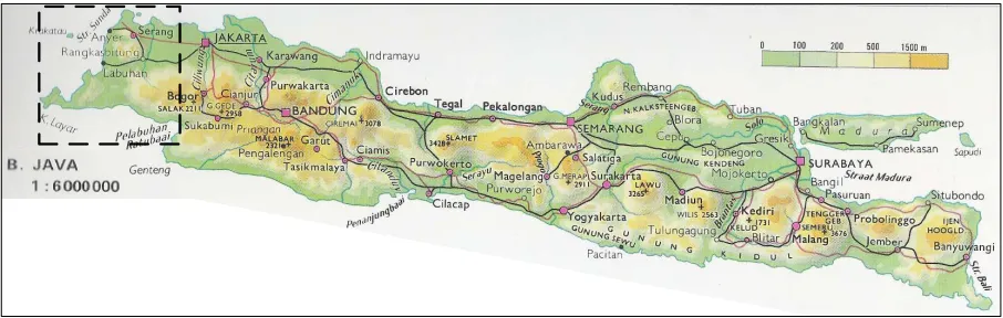
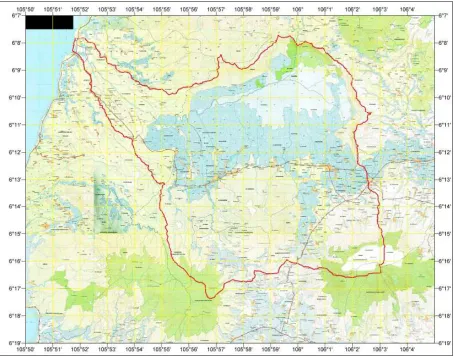
[image:12.595.71.524.214.358.2] [image:12.595.71.527.229.714.2]

The catchment used for this application in Indonesia is the watershed of the Cidanau River, which covers about 220 km2 (Buhdi et al., 2008). The river is located in the western part of Java, mainly in Serang regency (Banten Province) and partly in Pandeglang regency, see also figure 3.1 and 3.2.

Figure 3. 1: Location figure 3.2 on Java

(13)

[image:13.595.72.527.235.593.2]

The area is surrounded by several volcanic mountains and due to these mountains the water in the river keeps a certain height till it reaches a waterfall close to the coast. Formerly, there had been much more water in the area, because this area used to be a lake, but because of manually excavation of a channel besides the waterfall, most of the land (most of the darker blue area in figure 3.3 became dry and suitable for agriculture. Although there is less water in the region, the watershed still contains a lot of water, especially in the light blue area (figure 3.3), which mainly consists of swamp forest and swamp grass and is a nature protected area. This is the only remaining swamp area on Java and contains several endemic species (Shiozawa, 2004). The land-use in the area is presented in figure 3.4. From this picture can be concluded that most of the land is covered with rice, which tends to retain the available water as long as possible. Also the swamp area tends to keep water in the area for a long time.

Figure 3.3: Topographical map Cidanau.

The catchment is exposed to two seasons, a dry season from June to October and a wet season from November till May (Budhi, et al., 2008). During these periods the rainfall is 50 – 87 mm and 133 – 346 mm per month respectively to the dry and rainy season.

(14)

capacity of the pipe is 2,5m3/s , but the actual capacity is only 2,0m3/s (PT Krakatau Tirta

[image:14.595.71.389.113.380.2]

Industri, 2009) provided by three pumps.

Figure 3.4: Land-use Cidanau watershed (Rukzapol et al., 2006)

3.2 Data

De required data for this application are, as mentioned in chapter two, the climate data (i.e. precipitation and evapotranspiration) as input and the discharge data to calibrate and validate the model. The availability of these data during the years is shown in the time bar in Figure 3.5. In this picture the gaps in the data are shown in red. To calibrate and to validate the data, the data should not contain gaps, because the amount of water in the different response boxes depends on the situation in the past and without discharge data the output of the model cannot be compared. Eventually gaps could be filled with averaged values from the same periods in other years, but has not been used in this research. According to the split-sample test (Klemes, 1986) the nine years of data are divided into two parts that consist of complete years: a calibration period of five years and a validation period of four years. The available data before the calibration period is used as starting-up time, so that the amount of water in the soil moisture model box and in the upper and lower response boxes already depend on the past, before it is taken into account for the calculation of the R2 and the RVE. The starting values of

the validation period will be considered as the same as the end values of the calibration period and consequently does not need a start up time. The required data will be discussed here further to give a better understanding how the data are obtained.

[image:14.595.71.515.662.735.2]

(15)

3.2.1 Climate data

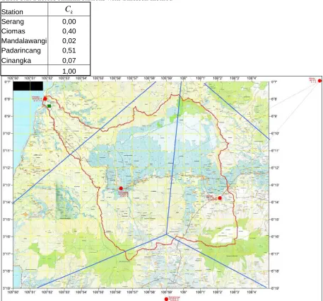
The rainfall data consists of 5 stations in the surrounding of the catchment: Cinangka, Ciomas, Mandalawangi, Padarincang and Serang. Two of these stations do not lie in the catchment and one is very close to the border near the sea. The result after applying the Thiessen method is shown in figure 3.5. This picture makes clear that, with applying the Thiessen method, the data from the Serang station should not be taken into account and that Cinangka and Padarincang have a very small influence on the calculated rainfall. This makes the rainfall mainly depending on only two stations. Therefore the calibration is also executed with an average rainfall over all the 5 stations. The coefficients C as defined in formula 2.4 _k

[image:15.595.69.526.252.677.2]

are shown in table 3.1.

Table 3.1: Factors rainfall stations with Thiessen method

Station Ck

Serang 0,00

Ciomas 0,40

Mandalawangi 0,02 Padarincang 0,51

Cinangka 0,07

1,00

Figure 3.6: Catchment with Thiessen method

(16)

kilometres from the centre of the catchment is almost the same. With this assumption the influence from different land heights is neglected.

3.2.2 Discharge data

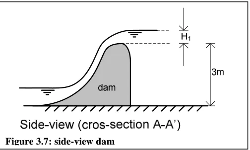
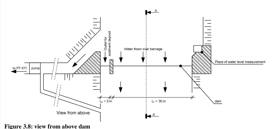
The discharge is measured at the dam that provides the water company with their water, which is located in the river 500 meters from sea (the green square in figure 3.5). The discharge consists of two parts which are measured separately, namely the part that is pumped to PT KTI and the part that is flowing over the dam and continues its way to the sea. The calculation of the first part is based on the number of pumps working at a certain moment. The second part is measured with a float and a connected mechanism that notes the water height at every moment on a paper. After one week the paper has to be refreshed, the discharge will be calculated with formula 3.1 and have to be entered into the computer manually.

(

3

)

2

1 1 2 2

3600 1, 705 0, 85

dam

Q = ⋅ ⋅H ⋅ +L ⋅H ⋅L (3.1)

The first part of this formula is for the water that is flowing over the dam itself, the second part stands for the water that is flowing over a small barrier which is used for sediment. H ₁

and H are the water height above the dam and the sediment barrier respectively (see figure ₂

3.7) and are assumed to be equal. L and₁ L are the width of the dam and the sediment barrier, ₂

see figure 3.8.

[image:16.595.73.325.420.571.2]

Unfortunately this way of measuring discharge introduces a lot of errors. In the first place the equation is determined after the beginning of the exploitation of the clean water in 1978 (PT Krakatau Tirta Industri, 2009), but may have become inaccurate, because of changes in the geometry of the river. Furthermore, because of the dam, the water is retained upstream and influences the discharge measurement close to the dam. Also the part of the water that goes to the water utilization is not accurate, because not all the water is measured. The main part is measured based on the number of pumps in operation, but partially it streams back to the river without going through the pump and being measured, see figure 3.8. During a normal hydrologic situation this error can be neglected, but during lower discharges the relative error increases. Furthermore, measuring the water height on paper causes errors, because the paper has a small margin, which makes it difficult and imprecise to determine the zero line of the water height. Finally making from this continuously measured graph a daily value is inexact because it is a human estimation based on the line on the paper.

(17)

O

u

tl

e

t

fo

r

se

d

im

e

n

t

d

e

p

o

si

[image:17.595.72.521.75.288.2]

t

(18)

4. Results and discussion

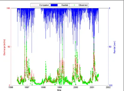
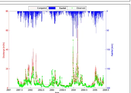
The predicted as well as the measured discharge of the Cidanau are presented in figure 4.1 and figure 4.2 for using the average rainfall and the rainfall determined with the Thiessen method respectively. This is the result of the calibration. The results for the validation are shown in figure 4.3 and figure 4.4 for the average rainfall and the rainfall from the Thiessen method respectively.

[image:18.595.73.489.197.503.2]

Table 4.1: result fitting criteria

Calibration Validation

Average Thiessen Average Thiessen

R2 [ - ] 0,71 0,73 0,64 0,60

RVE [%] -1,22 0,70 0,41 -1,96

The corresponding result of the fitting criteria R and RVE are displayed in table 4.1. From 2

this table it can be concluded that, although the R gives a reasonable result for the 2

calibration, although in this case the predicting ability of the model is not as accurate. An explanation can be found in the relatively short period of available data. According Bergstrom (1995) the model need five to ten years of data for calibration. The used five years could be sufficient, but a longer period may improve the result. For example, Lindström et al (1997) used ten years for calibration and ten years for verification. In the case that the climate data series can be extended till May 2009, it will be possible to use nine years of data for calibration and three years for validation, see figure 3.4. Three years of validation is very short, but because of an interruption in the data, it will be difficult to overcome this problem.

(19)

[image:19.595.69.524.71.371.2]

Figure 4.2: Comparison calculated and observed discharge of calibration with rainfall from Thiessen method

[image:19.595.73.525.400.720.2]

(20)

[image:20.595.72.523.70.373.2] [image:20.595.72.523.382.730.2]

Figure 4. 5: Zoom in discharge catchment Cidanau July 1999 – July 2000

(21)

From the graphs can be concluded that it is difficult to predict the discharge properly during extreme periods and these periods may for practical reasons be the most interesting part. This is made clearly visible from the detailed view in figure 4.5.

High peek values seem to be difficult. The model predicts a peek on the right moment, but the predicted discharge is often much too low. This can be caused by the spatially averaged precipitation that does not represent the real rainfall properly. On the other hand is the constant and relatively high discharge during dry periods not a realistic representation. This is caused by the base flow from the lower response box and is determined by the calibration parameters PERC andK . Changing the values of these parameters can make the situation ₄

during dry periods visually more realistic but decreases the value of the fitting criteriaR . 2

Considering the extreme situation without base flow from the lower response box (see figure 2.1) and calibrating again, the result converges toR2 =0, 69, which is less than the result obtained before (see table 4.1). The graph may give a more realistic visualisation for the dry periods of the years 2003 and 2004, but during the extremely dry period in 2002 the discharge goes to zero, as can be seen in figure 4.6.

[image:21.595.73.522.425.742.2]

The phenomenon of the base flow appears also in other models that are applied on the Cidanau catchment. For example, Setiawan and Rudiyanto (2004) applied another conceptual rainfall model, the Tank model, on the Cidanau River and compared this with other models. The tank model, which uses five in stead of three tanks as in the HBV model, has the same problems in times of low discharge. They examined that models with another type of model structure, for example the Storage Function model or the Artificial Neural Network model, can predict low discharge periods with much more accuracy and give as a result a higherR . 2

(22)

Further it is useful to compare the values of the calibration parameters with the limit values that Lidén and Harlin (2000) used during their automatic calibrations. The values are displayed in table 4.2. This table shows that the calibration process converges to values of FC (maximum soil moisture storage) and LP (limit for evapotranspiration) that largely exceeds the recommended upper limit. This difference of values could be explained by referring to the area. The main part of the area still consists of water retaining area, because for the production of rice it is important to keep the water as long as possible in the field and partially the catchment is covered by swamp. This means that a high value for FC could be expected. However, it is still questionable why the values using a different determined rainfall data lead to different values for FC, LP and

α

. Perhaps the found optimum is only a local optimum, because the parameters are highly interdependent. This is emphasised by the large differences between both spatially averaged rainfall methods in the values for FC. Using an automatic calibration as described in Harlin, (1991) and in Zhang and Lindström (1997) is therefore recommended for further applications to find the global optimum in an objective way.

A further explanation can be sought in the location of the discharge measurement, which is very close to the dam. Due to the dam the water is retained upstream. During the calibration this is compensated by high values of FC.

Table 4.2: range of values automatic calibration (Lidén and Harlin, 2000) and values after calibration manually.

range for automatic calibration Value after calibration Parameter Lower limit Upper limit Average rainfall Thiessen rainfall

FC (mm) 100 800 1430 3000

LP (mm) 50 100 581 1220

ß 1 6 1,00 1,00

CFLUX (mm/day) 0 1 0,00 0,00

α 0 3 0,758 0,675

PERC (mm/day) 0,1 5 2,70 2,80

[image:22.595.72.477.356.480.2]

(23)

5. Conclusions and recommendations

This simplified application of the HBV model gives a sound prediction for the discharge in the Cidanau with an Nash and Sutcliffe coefficient 2

R around 0,7. Most periods of the

prediction fits well with the measured discharge, but improvements can still be made for the extreme flow periods. During low flow periods the prediction is too high and unrealistically constant, because of a very constant modelled base flow. High discharge values appear usually in short periods and are therefore relatively unimportant in the fitting criteriaR , 2

despites the large errors in that period.

To improve the result furthermore it will be useful to use a longer calibration period than is used now. Because of the limited data availability and the presence of gaps in the data series, the calibration period is only five years. This is only the half of the recommended period by Berström (1995). Gaps can eventually be filled with average data from other years and excluded from the calculation of R2.

In addition the value of one calibration parameter is not realistic comparing with other researches (i.e. Lidén & Harlin, 2000). This might be caused by the manual calibration, which converges towards a local optimum. This could be solved by using an automatic calibration with a global optimisation algorithm as done by Zhang and Lindström (1997) and is therefore recommended for further applications. It will also be very useful for practical implementation in other areas to do further research to the exact physical meaning of certain parameter values. This will be useful for investigating consequences of practical changes in a certain area before implementation, for example to predict the consequences of decreasing retention capacity because of changes in land-use.

This unrealistic parameter can further be explained by the location of the discharge measurement. The discharge is measured just before the dam, but by the dam the water is retained upstream. For this situation the HBV model gets less robust, exhibited in this parameter value.

Furthermore, a distinction is made in the way of calculating the precipitation as input for the model, namely just taking the average and calculating the precipitation with the Thiessen method. After calibration of both data series the result does not show substantial differences in terms of the 2

R , although it is expected that the Thiessen method would represent the

(24)

References

Abbott, M.B., Bathurst, J.C., Cunge, J.A., O’Connell, P.E., & Rasmussen, J. (1986). An introduction to the European hydrological system – Système Hydrologique Européen, “SHE”, 1: history and philosophy of a physically-based, distributed modelling system.

Journal of Hydrology, 87, 45-59.

Allen, R.G., Luis, S.P., Raes, D., & Smith, M (1998). Crop evapotranspiration – Guidelines for computing crop water requirements – FAO Irrigation and drainage paper 56. Retrieved July 7, 2009, from FAO. Food and Agriculture Organization of the United Nations. Web site: http://www.fao.org/docrep/X0490E/x0490e00.htm#Contents. Bergström, S. (1995). The HBV model. In V.P. Sing, Computer models of watershed

hydrology, (pp. 443 – 476). Highland ranch, NJ: Water resources Publications.

Bergström, S., & Forsman, A. (1973). Development of a conceptual deterministic rainfall-runoff model. Nordic Hydrology, 4, 147 – 170.

Booij, M.J. (2005). Impact of climate change on river flooding assessed with different spatial model resolutions. Journal of Hydrology, 303, 176 – 198.

Budhi, G.S., Sa, K.,& Iqbal, M. (2008). Concept and implementation of PES program in the Cidanau watershed: a lesson learned for future environmental policy. Analisis

Kebijakan Pertanian, 6 (1), 37 – 55.

Carpenter, T.M., & Georgakakos, K.P. (2006), Intercomparison of lumped versus distributed hydrologic model ensemble simulations on operational forecast scales. Journal of

Hydrology, 329, 174-185.

Cruz, R.V., Harasawa, H., Lal, M., Wu, S., Anokhin, Y., Punsalmaa, B., Honda, Y., Jafari, M., Li, C., & Huu Ninh, N. (2007). In Climate Change 2007: Impacts, Adaptation and vulnerability. Contribution of working group 22 to the fourth assessment report of the intergovernmental panel on climate change, M.L. Parry, O.F. Canziani, J.P. van der Linden and C.E. Hanson (Eds.), Cambridge University Press, Cambridge, 469 – 506. Dirks, K.N., Hay, J.E., Stow, C.D., & Harris, D. (1998). High-resolution studies of rainfall on

Norfolk Island. Part II: Interpolation of rainfall data. Journal of Hydrology, 208, 187 – 193.

Graham, L.P., & Bergström S. (2001). Water balance modelling in the Baltic Sea drainage basin – analysis of meteorological and hydrological approaches. Meteorology and

Atmospheric Physics, 77, 45 – 60.

Harlin, J. (1991). Development of a process oriented calibration scheme for the HBV hydrological model. Nordic Hydrology, 22, 15 – 36.

Khoob, A.R. (2008). Comparing study of Hargreaves’s and artificial neutral network’s methodologies in estimating reference evapotranspiration in semiarid environment.

(25)

Klemes, V. (1986). Operational testing of hydrological simulation models. Hydrological

Sciences Journal, 31 (1), 13 – 24.

Lidén, R., & Harlin, J. (2000). Analysis of conceptual rainfall – runoff modelling performance in different climates. Journal of Hydrology, 238, 231 – 247.

Lindström, G., Johansson, B., Persson, M., Gardelin M., & Bergström, S. (1997). Development and test of the distributed HBV-96 hydrological model. Journal of

Hydrology, 210, 272 – 288.

Monteith, J.L. (1988). Does evapotranspiration limit the growth of vegetation of vice versa?

Journal of Hydrology, 100, 57 – 68.

Nash, J.E., & Sutcliffe I.V. (1970). River flow forecasting through conceptual models part 1 – A discussion of principles. Journal of Hydrology, 10, 282 – 290.

PT Krakatau Tirta Industri (2009). Expansion of the distribution piping network and

improvement of service to the costumers, our products. Retrieved 23 June from

http://www.krakatautirta.co.id./

Rukzapol, A., Lewandowska, A., Permana, E., Sumsuri, Yimsoi, T., Vihemäki, H., &

Watanakul, D.P. (2006). Land use map for Cidanau Watershed. Retrieved 1 July 2009 from http://www.forrsa.info/

Setiawan, B.I., Arief, Ch., Saptomo, S.K., Saritomo & Kusmayadi (2009). Impact of climate

changes on water resource in Cidanau watershed, Banden province Indonesia.

Unpublished manuscript.

Setiawan, B.I. & Rudiyanto (2004). Hydrological models for Cidanau watershed. Proceeding of third international seminar on harmonization between development and

environmental conservation in biological production. JSPS-DGHE core university program in applied biosciences. Banten, December 3-5, 2004.

Shiozawa, S., Katjita, N., Ishikawa, M., Goto, A., Sato, Y., Basa, E.R.,& Setiawan, B.I. (2004). Water level in Rawa Danau swamp in Cidanau watershed, at present and in

the past. Proceedings of the 3rd Seminar, Toward harmonization between development and environmental conservation in biological production, Serang, Banten (Indonesia).

Sivakumar, B. (2007). Dominant processes concept, model simplification and classification framework in catchment hydrology. Stoch Environ Res Risk Assess, 22, 737 – 748. Strzepek, K.M. & Yates, D.N. (1997). Climate change impacts on the hydrologic resources of

Europe: a simplified continental scale analysis. Climatic Change, 36, 79-92.

Todini, E. (1988). Rainfall-runoff modelling – Past, present and future. Journal of Hydrology,

100, 341-352.

(26)