Phase space formulation of the nonlinear longitudinal relaxation of the magnetization in quantum spin systems

Phase-space formulation of the nonlinear longitudinal relaxation of the magnetization

in quantum spin systems

Yuri P. Kalmykov,1 William T. Coffey,2and Serguey V. Titov2,3

1_{Laboratoire de Mathématiques, Physique et Systèmes, Université de Perpignan, 52, Avenue de Paul Alduy,}

66860 Perpignan Cedex, France

2

Department of Electronic and Electrical Engineering, Trinity College, Dublin 2, Ireland

3

Institute of Radio Engineering and Electronics of the Russian Academy of Sciences, Vvedenskii Square 1, Fryazino, 141190, Russian Federation

共Received 30 April 2007; revised manuscript received 18 June 2007; published 8 November 2007兲

Nonlinear longitudinal relaxation of a spin in a uniform external dc magnetic field is treated using a master equation for the quasiprobability distribution function of spin orientations in the configuration space of polar and azimuthal angles共analogous to the Wigner phase space distribution for translational motion兲. The solution of the corresponding classical problem of the rotational Brownian motion of a magnetic moment in an external magnetic field essentially carries over to the quantum regime yielding in closed form the dependence of the longitudinal spin relaxation on the spin sizeSas well as an expression for the integral relaxation time, which in linear response reduces to that previously given by D. A. Garanin关Phys. Rev. E 55, 2569共1997兲兴using the density matrix approach. The nonlinear relaxation is dominated by a single exponential having as time constant the integral relaxation time. Thus a simple description in terms of a Bloch equation holds even for the nonlinear response of a giant spin.

DOI:10.1103/PhysRevE.76.051104 PACS number共s兲: 05.40.⫺a, 03.65.Yz, 76.20.⫹q

I. INTRODUCTION

Spin relaxation is fundamental in the physics and chem-istry of condensed phases, e.g., on anatomiclevel, nuclear magnetic and related spin resonance experiments probe the time evolution of the elementary spins of nuclei, electrons, muons, etc. 关1,2兴. On a larger scale the time evolution of magneticmolecular clustersexhibiting relatively large quan-tum effects关3兴 with spins of order 15– 25␮B is currently of interest in the context of molecular magnets. Finally, on a

nanoscalelevel, we have magnetic fluids composed of single domain ferromagnetic particles 共constituting a single giant spin of magnitude 104_{– 10}5_{␮B兲 in a colloidal suspension.} Here relaxation experiments detect关4,5兴both the Arrhenius or solid-state-like共Néel兲mechanism关6兴of relaxation of the magnetization, which may overcome via thermal agitation anisotropy, potential barriers inside the particle and the De-bye共or Brownian兲relaxation关7兴due to physical rotation of the suspended particles in the presence of an applied field and the heat bath. Here quantum effects are expected to be much smaller.

Spin relaxation experiments in nuclear magnetic or elec-tron spin resonance are usually interpreted via the phenom-enological Bloch关8兴 equations and their later modifications 关1,2兴. They describe relaxation of an assembly of elementary spins in a sample subjected to an external magnetic field and coupled to a heat bath. These simple linear equations of mo-tion for the nuclear magnetizamo-tion were originally proposed on phenomenological grounds. The main assumption is that the effects of the heat bath can be described by two time constants, the so-called relaxation times. They provide a sub-stantially correct 关1兴 quantitative description for liquid samples. Microscopic theories of the relaxation in quantum spin systems have been developed by Bloembergen, Purcell, and Pound关9兴, and other authors共see, e.g.,关10–12兴兲.

Proceeding to larger scales, in magnetic molecular clus-ters comprising a few spins the relaxation behavior as a func-tion of spin is of paramount importance as strong quantum effects are expected to manifest themselves as the spin de-creases, while in single domain 共giant spin兲 nanoparticles suspended in a fluid carrier the relaxation is usually assumed to be classical. Thus the Néel mechanism of the magnetiza-tion reversal关6兴occurring inside the ferromagnetic particles is described by a classical Langevin equation for the time evolution of the magnetization as adapted to magnetic mo-ments by Brown关13,14兴 while the Debye theory 关7兴 of di-electric relaxation of polar molecules is used to describe the relaxation by physical rotation of the suspended particles 关4,15兴. In the description of the Néel mechanism关13,14兴, the Langevin equation is the phenomenological Landau-Lifshitz 关16兴 or Gilbert equation 关17兴 for the magnetization M共t兲

exhaustively compared 关5兴 with exact solutions yielded by the Fokker-Planck equation. Now it has been suggested by Bean and Livingston关25兴that in addition to the overbarrier relaxation mechanism mentioned above the magnetization may also reverse by quantum tunneling through the barrier. This relaxation mechanism representsmacroscopic quantum tunnelingsince a giant spin is always involved关26兴.

These considerations merit a systematic way of introduc-ing quantum effects into the spin dynamics simultaneously linking to the classical representation and allowing one to study quantum effects. The method proposed here utilizes the coherent state representation of the density matrix introduced by Glauber and Sudarshan commonly used in quantum op-tics 共see, e.g., 关27,28兴兲. This method when applied to spin systems 关29,30兴allows one to analyze quantum spin relax-ation using a master equrelax-ation for aquasiprobability distribu-tion funcdistribu-tion W␴共␽,␸,t兲of spin orientations in a phase共here configuration兲 space 共␽,␸兲; ␽ and␸ are the polar and azi-muthal angles, constituting the canonical variables. Here␴ parametrizes quasiprobability functions of spins belonging to the SU共2兲rotation group, and␴= 0 and␴= ± 1 correspond to the Stratonovich关31兴and Berezin关32兴contravariant and co-variant functions, respectively共the latter are directly related to theP andQ symbols, which appear naturally in the co-herent state representation; see Refs.关33,34兴for a review and Appendix A for details. We considerW−1_{共␽,␸,t兲 only and} drop the superscript. Such a mapping of the quantum spin dynamics ontoc-number quasiprobability density evolution equations clearly shows how these reduce to the Fokker-Planck equation in the classical limit 关29,30兴. The function

W共␽,␸,t兲was originally introduced by Stratonovich关31兴for zero dissipation, i.e., for closed systems, and further devel-oped both for closed and open spin systems 共e.g., 关29,30,32–42兴 and is entirely analogous to the translational Wigner distribution W共x,p,t兲 in phase space 共x,p兲 关43兴, which is the quasiprobability representation of the density operator except that certain differences arise关29兴because of the angular momentum commutation relations. The Wigner function W共␽,␸,t兲 of spin orientations in a configuration space, just as the Wigner functionW共x,p,t兲 for the transla-tional motion of a particle in phase space, enables the ex-pected value具Aˆ典共t兲 of a quantum spin operatorAˆ to be cal-culated via the corresponding共c number兲 function A共␽,␸兲. For example, for the spin operator SˆZ, the correspondence rules of operators and c numbers yield SˆZ→共S+ 1兲cos␽, while the expected value具SˆZ典共t兲is

具SˆZ典共t兲=2S+ 1 4␲

冕

₀

␲

冕

0 2␲

共S+ 1兲cos␽W共␽,␸,t兲sin␽d␽d␸

共see Appendix A for details兲. The phase-space formalism al-lows quantum mechanical averages involving the density matrix to be calculated just as classical ones and so is emi-nently suited to the calculation of quantum corrections be-cause it formally represents quantum mechanics as a statis-tical theory on classical phase space 关44兴. Indeed W共x,p,t兲

has been recently used 关45–48兴 for quantum corrections to the classical theory of the translational Brownian motion via

perturbation theory inប2 _{共ប is Planck’s constant兲. The} for-malism is easy to implement because semiclassical master equations in phase space enable techniques共e.g., continued fractions 关49兴兲 originally developed for the solution of the Fokker-Planck equation to be seamlessly carried over into the quantum domain关45,47兴. In particular共which is relevant in the present context兲, we note the semiclassical quantum master equation in phase space for the translational harmonic quantum oscillator in the weak coupling limit 共originally studied by Agarwal关50兴兲

⳵W

⳵t +

p m

⳵W

⳵x −m␻0

2

x⳵W

⳵p =

␵

m

⳵

⳵p

冋

pW+具p

2_典eq⳵W

⳵p

册

, 共1兲

where ␵, m, and ␻0 are the “friction” coefficient, mass, and oscillator frequency, respectively, 具p2_典eq =共mប␻0/ 2兲coth共␤ប␻0/ 2兲,␤= 1 /共kT兲, andkTis the thermal energy. Equation共1兲is the same as the Fokker-Planck equa-tion 共here the Klein-Kramers equation兲 for a classical Brownian oscillator 关5兴 except the diffusion coefficientDpp =␵具p2典eq/mis altered to include the quantum effects. Thus it is unnecessary to resort to perturbation theory because the dynamical equation for the Wigner function for a quadratic HamiltonianHˆ=pˆ2_{/ 2m+m␻}

0

2_xˆ2_{/ 2 in the absence of} dissipa-tion共␵= 0兲coincides with the corresponding classical Liou-ville equation.

Now for a spin in an external uniform field if the coherent state representation is transferred to the conventional polar and azimuthal angle representation共␽,␸兲, the master equa-tion describing the time evoluequa-tion of W共␽,␸,t兲 again has essentially the same form as the corresponding classical Fokker-Planck equation 关30兴. Hence the problem is analo-gous to the Agarwal harmonic oscillator model 关50兴 thus serving as the most simple example of the application of the phase-space method to open spin systems 关29,30,41,42兴 as we demonstrate here. We remark that the master equation has been solved by continued fractions in Ref.关41兴 for the lon-gitudinal relaxation for particular small values of the spin

S= 1 / 2, 1, and 3 / 2. Here we shall present both theexactand an approximate general solution for the linear andnonlinear

relaxation of the averaged longitudinal component of the spin具SˆZ典共t兲 as a function of all spin valuesS in a uniform magnetic field ofarbitrarystrength. We shall show how the solution of the corresponding classical problem 关5,51–54兴

carries over into the quantum domain and how the exact solution for the integral relaxation time for an arbitrarily strongchange in the uniform field may be obtained. In the

linear response approximationthe exact solution reduces to that previously given by Garanin关55兴using the spin density matrix in the second order of perturbation theory in the spin bath coupling and later rederived by García-Palacios and Zu-eco关56兴who共again using the density matrix兲considered the linear longitudinal relaxation for arbitrary S. Furthermore, we shall demonstrate that the relaxation of the spin具SˆZ典共t兲, comprising 2S exponentials, may be accurately approxi-mated by asingleexponential with a definite relaxation time

arbitrary S. In other words, even for a giant spin 共SⰇ1兲, 具SˆZ典共t兲still obeys the Bloch equation

d

dt具SˆZ典共t兲+共具SˆZ典共t兲−具SˆZ典eq兲

Ⲑ

T1= 0, 共2兲

where具SˆZ典eq is the equilibrium average of the operatorSˆZ. We remark in passing that Garanin and García-Palacioset al.

关55–57兴evaluated the response for a more general spin sys-tem 共a uniaxial paramagnet in a uniform field兲. They have given a quantum treatment of the spin dynamics by proceed-ing from the quantum Hubbard operator representation of the evolution equation for the spin density matrix. However, they considered asmall longitudinal ac field superimposed on a longitudinal dc field so that by linear response theory their solution is strictly limited to the response consequent on a small perturbation in the dc field unlike ours, which is valid for arbitrary changes in the dc field, thus no longer necessar-ily bearing any relation to the ac response.

II. BASIC EQUATIONS FOR THE LONGITUDINAL RELAXATION

Following关30,41,42兴we consider the dynamics of a spin Sˆ in an external dc magnetic field H0 directed along the Z axis and a random field h共t兲 characterizing the collision damping共due to the heat bath兲incurred by the precessional motion of the spin so that the HamiltonianHˆ is

Hˆ =HˆS+HˆSB+HˆB,

whereHˆS= −ប␻0SˆZ,␻0=␥H0is the precession共Larmor兲 fre-quency,␥ is the gyromagnetic ratio, the termHˆSB= −ប␥h·Sˆ describes interaction of the spin with the thermostat, andHˆB characterizes the thermostat. The equation of motion for the density matrix␳ˆ is then

⳵␳ˆ

⳵t +

i

ប关HˆS,␳ˆ兴=Qˆ共␳ˆ兲, 共3兲 whereQˆ共␳ˆ兲= −共i/ប兲关HˆSB+HˆB,␳ˆ兴 is the collision kernel op-erator. The reduced density matrix␴ˆ= TrB␳ˆ 共i.e., that aver-aged over the density matrix of the bath兲obeys the following equation关30兴:

⳵␴ˆ

⳵t =i␻0关Sˆ0,␴ˆ兴+B

*_e␤ប␻0关_Sˆ

+␴ˆ,Sˆ−兴+Be␤ប␻0关Sˆ+,␴ˆ Sˆ−兴 +B关Sˆ−␴ˆ,Sˆ+兴+B*关Sˆ−,␴ˆ Sˆ+兴+C关Sˆ0␴ˆ,Sˆ0兴+C*关Sˆ0,␴ˆ Sˆ0兴, whereSˆ₊,Sˆ₋, and Sˆ₀=SˆZare the spin operators in spin co-herent state representation共defined in Ref.关30兴兲and

B=共␥/2兲2

冕

0 ⬁

具h−共t兲h+共0兲典Be−i␻0t_dt,

C=␥2

冕

0 ⬁

具h0共t兲h0共0兲典Bdt.

Here the averages are over the equilibrium bath density ma-trix共assuming axial symmetry about theZaxis and that the averaged field components 具h±_{共t兲典B= 0 and 具h}0_{共t兲典B= 0兲. In} the longitudinal relaxation, the azimuthal dependence ofW

may be ignored so that the corresponding evolution equation forW共␽,t兲is关30兴

⳵W

⳵t =

b共e␤ប␻0_{− 1}兲

sin␽

⳵

⳵␽

再

共sin␽关coth共␤ប␻0/2兲+ cos␽兴兲

⳵W

⳵␽

+ 2Ssin2␽W

冎

, 共4兲

where b= Re共B兲 is the effective “diffusion” coefficient re-lated to the random magnetic field imposed by the reservoir on the spin. Equation共4兲applies in the narrowing limit case when the correlation time␶cof the random field h共t兲acting on the spin satisfies the condition␥H␶cⰆ1, where His the averaged amplitude of the random magnetic field. The left hand side of Eq.共4兲is the quantum analog of the Liouville equation for a spin, which in this instance is the same as the classical case just as the corresponding result for particles with quadratic Hamiltonians, while the right hand side共 col-lision kernel兲 characterizes the interaction of the spin with the thermal bath at temperatureT. Conditions for the validity of Eq.共4兲are discussed in detail elsewhere共see, e.g.,关30兴兲. Essentially, Eq. 共4兲 follows from the equation of motion of the reduced density matrix where the interactions between the spin and the heat bath are small enough to allow one to use the weak coupling limit and the correlation time charac-terizing the bath is so short that we can regard the stochastic process originating in the bath as Markovian关30兴. Thus one may assume frequency independent damping. This approxi-mation may be used in the high temperature limit. In the parameter range, where such an approximation is invalid 共e.g., throughout the very low temperature region兲, a more general form of the master equation with time dependent diffusion coefficients关41,42兴should be used. We have cho-sen Eq. 共4兲 in the approximation of frequency independent damping because our objective is merely to understand in semiclassical fashion how quantum effects alter the rota-tional Brownian motion and nonlinear longitudinal relax-ation of a classical spin. We also remark that in the case of longitudinal relaxation, Eq.共4兲may be plausibly derived共see Appendix B兲by postulating共just as in the phase space treat-ment of the quantum translational Brownian motion关46,48兴兲

a master equation for the Wigner functionW with collision terms given by a Kramers-Moyal expansion truncated at the second term. The various drift and diffusion coefficients in the truncated expansion may then be calculated by requiring that the equilibrium Wigner distributionWeq, corresponding to the equilibrium spin density matrix␳ˆ_eq=e−␤HˆS_{/ Tr}兵_e−␤HˆS其_,

renders the collision kernel equal to zero.

Weq共␽兲=ZS−1

冋

cosh

冉

1

2␤ប␻0

冊

+ sinh

冉

1

2␤ប␻0

冊

cos␽

册

2S

, 共5兲

where

ZS=

冉

S+ 1 2

冊

冕

₋₁

1

冋

cosh

冉

1

2␤ប␻0

冊

+ sinh

冉

1

2␤ប␻0

冊

z

册

2S

dz

= sinh

冋

冉

S+1

2

冊

␤ប␻0

册

冒

sinh

冉

1 2␤ប␻0

冊

is the partition function. The average longitudinal component of the spin at equilibrium is

具SˆZ典eq=

冉

S+1 2

冊

冕

0

␲

共S+ 1兲cos␽Weq共␽兲sin␽d␽

=SBS共␤ប␻0S兲, 共6兲

whereBS共x兲 is the Brillouin function defined as关49兴

BS共x兲= 2S+ 1 2S coth

冉

2S+ 1 2S x

冊

−

1 2S coth

冉

x

2S

冊

. 共7兲

Equation共6兲is in complete agreement with the well-known result for the equilibrium magnetization of a spin in a uni-form magnetic field 关58兴. In the classical limit, ␤→0, S

→⬁, and␤S= const, the equilibrium distributionWeq共␽兲and the Brillouin functionBS共x兲tend, respectively, to the Boltz-mann distribution, i.e.,

共

S+1₂

兲

Weq共␽兲→Z_cl−1eS␤ប␻0cos␽_{, and}

the Langevin function, i.e., BS共x兲→L共x兲= coth共x兲− 1 /x, whereZclis the classical partition function. Quantum effects become important whenប␥H₀/共kTS兲艌1, i.e., either at small

Sor at very low temperaturesTor for an intense fieldH₀.

III. EXACT SOLUTION OF THE MASTER EQUATION (4)

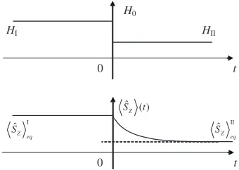
We suppose that the magnitude of an externally uniform dc magnetic field is suddenly altered at timet= 0 fromHIto HII共the magnetic fieldsHIandHIIare assumed to be applied parallel to the Z axis of the laboratory coordinate system兲. Thus we study as in the classical case 关5,59兴 the transient longitudinal relaxation of a system of spins starting from an equilibrium state I with the distribution functionW_eqHI 共_t艋₀兲

to a new equilibrium state II with the distribution function

W_eqHII 共_t→⬁兲_{. Here the longitudinal component of the spin}

具SˆZ典共t兲relaxes from the equilibrium value具SˆZ典_eqI to the value 具SˆZ典_eqII, the transient being described by an appropriate relax-ation function共see Fig.1兲. The transient response so formu-lated is truly nonlinear because the change in amplitudeHI −HIIof the external dc magnetic field isarbitrary共the linear response can be treated as the particular case兩HI−HII兩→0兲. The master equation共4兲for the evolution ofW共z,t兲 共with

z= cos␽兲 can be given in the form of a single variable Fokker-Planck equation fort⬎0 关30兴,

⳵W

⳵t =

⳵

⳵z

冉

D

共2兲_共z兲⳵

⳵zW−D

共1兲_共z兲W

冊

_{, 共8兲} whereD共1兲共z兲andD共2兲共z兲are, respectively, the drift and dif-fusion coefficients given by

D共1兲共z兲=S共e␰/S− 1兲共1 −z2兲/共2␶N兲, 共9兲

D共2兲_共z兲=共e␰/S_{+ 1兲关1 +ztanh共␰/2S兲兴共1 −z}2_{兲/共4␶N兲,} 共10兲

␶N= 1 /共4b兲 is the characteristic time of the free rotational “diffusion” of the spin, and the dimensionless field parameter

␰is defined as

␰=␤ប␥H_IIS. 共11兲

We remark that the explicit form ofD共1兲_共z兲andD共2兲_{共z兲can be} obtained from the Fokker-Planck equation共8兲using the equi-librium distribution Eq.共5兲 alone exactly as in the transla-tional Brownian motion关48兴 共see Appendix B兲.

The solution of Eq.共8兲is obtained by expanding the dis-tribution functionW共z,t兲in a series of Legendre polynomials

Pn共z兲

W共z,t兲=W_eq␰共z兲+

兺

n=0 2S

2n+ 1

2S+ 1Pn共z兲fn共t兲, 共12兲

where the equilibrium distributionW_eq␰共z兲is defined as关c.f., Eq.共5兲兴

W_eq␰共z兲=ZS −1_关

cosh共␰/2S兲+ sinh共␰/2S兲z兴2S

=

兺

n=0 2S

2n+ 1

2S+ 1Pn共z兲具Pn典eq

␰ _{, 共13兲}

and

具Pn典_eq␰ =

冉

S+1 2

冊

冕

₋₁

1

Pn共z兲W_eq␰共z兲dz 共14兲

is the equilibrium average of Pn共z兲. In particular, we have 具P1典_eq␰ =关S/共S+ 1兲兴BS共␰/S兲. Substituting Eq.共12兲into Eq.共8兲

and noting the orthogonality and recurrence properties of the Legendre polynomials 关60兴 as in the classical case 关5兴 we

0 t

H0

HII HI

II ˆ

Z _eq

S

ˆ _{( )}

Z

S t

0 t

I ˆ

Z _eq

[image:4.612.352.522.60.181.2]

S

have a differential-recurrence relation for the relaxation functionsfn共t兲=具Pn典共t兲−具Pn典_eq␰, viz.,

␶nf˙n共t兲=qn−fn−1共t兲+qnfn共t兲+qn+fn+1共t兲, 共15兲 where 1艋n艋2S, f0共t兲=f2S+1共t兲= 0,

␶n= 2␶N/关n共n+ 1兲兴, qn= −共1 +e␰/S兲/2,

qn ±

= ⫿2S±n+共3 ± 1兲/2 2共2n+ 1兲 共e

␰/S_{− 1兲,}

and the brackets具 典共t兲designate statistical averaging defined as具䉺典共t兲=

共

S+1₂

兲

兰₋₁1 䉺W共z,t兲dz.

Using the properties of the one-sided Fourier transform, we have from Eq.共15兲

共i␻␶n−qn兲f˜n共␻兲−qn −

f˜n−1共␻兲−qn +

f˜n+1共␻兲=␶nfn共0兲, 共16兲

where f˜n共␻兲=兰₀⬁e−i␻t_{fn共t兲dt. The inhomogeneous three-term} recurrence Eq. 共16兲 can be solved exactly for f˜1共␻兲 using continued fractions just as the corresponding classical prob-lem共see for details Ref.关5兴, Chap. 2兲yielding

f˜1共␻兲= 2␶N 共e␰/S− 1兲

兺

_n=1

2S

an

兿

k=1 n

⌬k

储_共␻

,␰兲. 共17兲

Here the finite continued fraction⌬n

储_共␻

,␰兲 is defined by the recurrence relation

⌬n

储_共␻

,␰兲=qn−关i␻␶n−qn−qn+⌬n+1

储 _共␻

,␰兲兴−1, with⌬_2S+1储 共␻,␰兲= 0 and

an=

fn共0兲

n共n+ 1兲共S+ 1兲

兿

k=1 n

q_k−1+ qk−

=共− 1兲n+1fn共0兲共2n+ 1兲共2S+n+ 1兲!共2S−n兲!

n共n+ 1兲共S+ 1兲共2S+ 1兲!共2S兲!. Noting that the initial value for the distribution function is

W共z, 0兲=W_eq␰+␦共z兲, where ␦=␤ប␥S共HII−HI兲 共that is, the per-turbation strength兲, the initial values for the fn共t兲are

fn共0兲=具Pn典_eq␰+␦−具Pn典_eq␰ . 共18兲 The equilibrium averages具Pn典_eq␰ given by Eq. 共14兲 can also be evaluated in terms of ⌬_n储共0 ,␰兲 since 具Pn典eq␰ satisfies the three-term recurrence relation

qn−具Pn−1典eq␰ +qn具Pn典eq␰ +qn+具Pn+1典eq␰ = 0, 共19兲 so that⌬n

储_共

0 ,␰兲=具Pn典_eq␰ /具Pn−1典_eq␰ and 具Pn典_eq␰ =

兿

k=1 n

⌬k

储_共

0,␰兲. 共20兲

Equation共17兲is the exact solution for the one-sided Fou-rier transform of the nonlinear relaxation function f1共t兲 in terms of continued fractions. Having determined f1共t兲, vari-ous transient nonlinear responses of the longitudinal

compo-nent of the normalized magnetization 具MˆZ典共t兲=具SˆZ典共t兲

−具SˆZ典_eq␰ may be evaluated because

具MˆZ典共t兲=共S+ 1兲f1共t兲, 共21兲 where 具SˆZ典_eq␰ =SBS共␰/S兲. In particular, we mention the rise, decay, and rapidly reversing field transient responses. In some cases, the general equation 共17兲 can be considerably simplified. For example, let us now suppose that a strong constant fieldHII is suddenly switched on at time t= 0 共so thatH_I=0or␦= −␰兲. Thus we are interested in the nonlinear relaxation of a system of spins starting from an equilibrium state I with the isotropic distribution function W_eq0 =共2S

+ 1兲−1 _{共t艋0兲 to another equilibrium state II with the} distri-bution function W_eq␰ 共t→⬁兲. Noting Eq. 共20兲, Eq. 共17兲 be-comes

f˜1共␻兲=i关⌬₁储共0,␰兲−⌬₁储共␻,␰兲兴/␻. 共22兲 Equation共22兲allows one to easily calculatef˜1共␻兲for the rise transient.

IV. NONLINEAR LONGITUDINAL RELAXATION TIME

The overall transient behavior of the relaxation function

f1共t兲 关hence the magnetization 具MˆZ典共t兲兴 is characterized by the integral relaxation time 关the area under the normalized relaxation functionf1共t兲/f1共0兲兴 关5兴

␶int= 1

f1共0兲

冕

₀ ⬁

f1共t兲dt= f˜1共0兲

f1共0兲, 共23兲 where f1共0兲=关BS共␰+␦兲−BS共␰兲兴S/共S+ 1兲. This time can be evaluated from Eqs.共17兲and共20兲and is given by

␶int=

2␶N 共e␰/S− 1兲f1共0兲

兺

_n=1

2S

an具Pn典eq␰. 共24兲

This expression can also be presented in an equivalent inte-gral form by noting that the master equation共8兲has the form of a single variable Fokker-Planck equation. As shown in Refs. 关5,59兴, for any system, with dynamics governed by a single variable Fokker-Planck equation, e.g., Eq.共8兲, the in-tegral relaxation time␶_intcharacterizing the nonlinear relax-ation behavior of f1共t兲=具P1典共t兲−具P1典_eq␰ can be obtained in closed integral form共just as for linear response兲in terms of the equilibrium distribution and the diffusion coefficient

D共2兲_{共z兲 only. Hence on applying these results to Eq.共8兲, we} obtain just as in the classical case关5,59兴the exact equation for␶int, viz.,

␶int=

共S+ 1/2兲

f1共0兲

冕

₋₁

1 _⌽共

z兲⌿共z兲

D共2兲共z兲W␰_eq共z兲dz, 共25兲

where ⌿共z兲=兰₋₁z 共x−具P1典_eq␰兲W_eq␰共x兲dx and⌽共z兲=兰₋₁z 关W_eq␰+␦共x兲

−W_eq␰共x兲兴dx. For the limiting caseS= 1 / 2,␶_intis independent of the perturbation strength␦ and is given by

␶int= 2␶N/共e2␰+ 1兲, 共26兲

␶int= 2␶N

f1共0兲

冕

−1 1 _␾共

z兲␺共z兲e−␰z

1 −z2 dz, 共27兲

where ␾共z兲=兰₋₁z 关W_cl␰+␦共x兲−W_cl␰共x兲兴dx, ␺共z兲=兰₋₁z 共cosz

⬘

−具P1典␰兲e␰z⬘dz

⬘

,f1共0兲=具P1典␰−具P1典␰+␦,具P1典␰= coth␰− 1 /␰, and

W_cl␰共z兲=␰e␰z/共2 sinh␰兲, agreeing entirely with the classical result关59兴.

Numerical calculations show that both Eqs.共24兲and共25兲

yield exactly the same result. Thus␶intfor various nonlinear transient responses 共such as the rise, decay, and rapidly re-versing field transients兲 may be easily evaluated from Eq. 共25兲. The normalized relaxation time␶int/␶Nfrom Eq.共25兲is shown in Fig.2as a function ofSand␰for various values of

␦. The figure indicates that the relaxation time decreases with increasing field strength␰ and, moreover, strongly depends onboth Sand␦. The nonlinear effect comprising accelerated relaxation in the external field also exists for classical dipoles 关5,59兴. An explanation may be given as follows. In the ab-sence of the fieldH_II共␰= 0兲, the relaxation time of the spin is the free diffusion relaxation time␶N, viz.,␶int=␶N. In a strong field共␰Ⰷ1兲andSⰇ1, the relaxation time is determined by the damped diffusion of the spin in the field HII and the characteristic frequency is now the frequency of the spin oscillation aboutHII共in the vicinity ofz= 0兲, which is deter-mined by the inverse of the field induced probability current ⬃2D1共0兲=␰/␶N so that ␶int⬃␶N/␰. This asymptotic formula may be used to estimate␶intfor ␰Ⰷ1 and␦⬎0 and兩␦兩Ⰶ␰. The influence of the parameter␦, which enters into the inte-gral relaxation time due to the initial distribution function

W_eq␰+␦, is more pronounced for negative values of␦ and field strengths␰⬃2 – 7共see Fig. 2兲. For ␦⬃−␰, a more accurate formula is given by␶int⬃␶N/关␰− 1 −␰共␰+␦兲兴. The enhanced dependence of␶inton ␦ for negative values of␦ can be un-derstood because these cases correspond to rise and rapidly

reversing transients, where the initial and final distributions differ considerably. As far as thespin dependence of ␶int is concerned,␶intsubstantially depends onS共due to the strong spin dependence of the field induced probability current兲and is given for␰Ⰷ1 and␦⬎0 and兩␦兩Ⰶ␰共where the␦ depen-dence of the relaxation time may be ignored in the first ap-proximation兲by,

␶int⬃ 关2D1共0兲兴−1=共␶N/S兲共e␰/S− 1兲−1. 共28兲 This asymptote is also shown in Fig.2 共see also Fig.3兲.

V. LINEAR RESPONSE

We may also evaluate thelinear responseof a spin system to infinitesimally small changes in the magnitude of the dc field, which is of particular interest as the corresponding in-tegral relaxation time becomes the correlation time, which we stress has already been evaluated关55–57兴using the spin density matrix. Thus we again suppose that the uniform dc fieldHII is directed along theZ axis of the laboratory coor-dinate system and that a small probing fieldH1共H1储HII兲 hav-ing been applied to the assembly of spins in the distant past 共t= −⬁兲so that equilibrium conditions are fulfilled at timet

= 0, is switched off at t= 0. Here ␦→0 and f1共t兲/f1共0兲 re-duces to the normalized longitudinal dipole equilibrium cor-relation functionC储共t兲 关61兴, that is,

lim ␦→0

f1共t兲

f1共0兲=C储共t兲=

␤−1

␹储

冕

0 ␤

具MˆZ共−i␭ប兲MˆZ共t兲典eq␰d␭, 共29兲 where␹储 is the static susceptibility defined as

␹储=␤−1

冕

0 ␤

具MˆZ共−i␭ប兲MˆZ共0兲典_eq␰d␭=S2 ⳵

⳵␰BS共␰兲 共30兲

and

S2⳵

⳵␰BS共␰兲=

1 4

冋

csch

2

冉

␰

2S

冊

−共2S+ 1兲

2_csch2

冉

2S+ 1 2S ␰

冊

册

.

According to linear response theory共see, e.g.,关61兴兲, having determined the one-sided Fourier transform C˜储共␻兲

0 5 10

0.0 0.5 1.0

10 20

0.0 0.1 0.2 0.3

3 4

1

S= 10 1:δ= 10 2:δ= 0 3:δ=−5 4:δ=−10

τ

int

/

τ

N

ξ

2

(b)

2 3 4

1

τ

int

/

τ

N

ξ= 5

1:δ= 5 2:δ= 0 3:δ=−2 4:δ=−4

S

1/2

[image:6.612.72.275.59.275.2]

(a)

FIG. 2. 共Color online兲 Normalized integral relaxation time

␶int/␶N from Eq.共25兲as a function of S共a兲 and ␰共b兲for various

values of␦共symbols兲. Dashed line: Eq.共28兲.

0 5 10

10−2 10−1

100

2 3 4

1

1:S= 1 2:S= 3 3:S=10 4:S→ ∞

ξ

τ cor

/

τ N

FIG. 3.共Color online兲Normalized correlation time␶cor/␶Nfrom

[image:6.612.355.522.60.187.2]

=兰0⬁C储共t兲e−i␻tdt 关the spectrum of the equilibrium correlation

functionC储共t兲兴, one may evaluate the dynamic susceptibility ␹储共␻兲=␹

⬘

储共␻兲−i␹

⬙

储共␻兲 关61兴via

␹储共␻兲/␹储= 1 −i␻C˜储共␻兲. 共31兲

In the linear response approximation, the integral relaxation time, that is, the correlation time 兩␶int兩_␦→0=␶_cor=C˜储共0兲 of

C储共t兲, follows from Eq.共25兲 in the limit␦→0 and is given

by

␶cor=

共S+ 1兲共S+ 1/2兲

S⳵BS共␰兲/⳵␰

冕

−1 1

1

D2共z兲W_eq␰共z兲

冕

₋₁

z

⳵

⳵␰Weq␰共x兲dx

⫻

冕

−1 z

冉

y−SBS共␰兲

S+ 1

冊

Weq

␰_{共y兲dydz, 共32兲}

where

⳵

⳵␰Weq␰共z兲=

csch共␰/2S兲−共2S+ 1兲csch共␰+␰/2S兲共cosh␰−zsinh␰兲 2S关cosh共␰/2S兲+zsinh共␰/2S兲兴 Weq

␰_共z兲.

For the limiting case S= 1 / 2, ␶cor is equal to ␶int from Eq. 共26兲, while in the limitS→⬁,

␶cor=

␶N␰csch␰

1 +␰−2− coth2␰冕−1 1

关z− coth␰+e−␰共1+z兲共1

+ coth␰兲兴2e ␰z

dz

1 −z2, 共33兲

agreeing entirely with the classical result共关5兴, Chap. 7兲. In the low field limit 共␰Ⰶ1兲, the correlation time may be ap-proximated as ␶cor/␶N= 1 −␰/共2S兲+O共␰2兲; in the classical limit S→⬁, one has 关5兴 ␶cor/␶N= 1 −␰2/ 9 +O共␰4兲. As far as the spin and field dependence of␶corfor␰Ⰷ1 is concerned, a simple asymptotic formula for␶cor=兩␶int兩␦→0 is given by Eq. 共28兲. It varies smoothly from the power law共␶cor⬃␶N/␰兲 at

S→⬁to exponential decrease共␶_cor⬃2␶Ne−2␰兲atS= 1 / 2. The qualitative behavior of ␶_cor=兩␶int兩_␦→0 has been discussed in Sec. IV. The normalized correlation time ␶cor/␶N from Eq. 共32兲is plotted in Fig.3as a function of␰for various values ofS; the asymptotes from Eq.共28兲 are also shown here for comparison.

We remarked above that the linear response had been studied previously by Garcia-Palacios and Zueco关56兴using the spin density matrix approach. They also gave an explicit expression for the linear response integral relaxation time first derived by Garanin 关55兴. Garanin derived his formula for a more general Hamiltonian than that treated in the present paper, namely, that corresponding to a uniaxial para-magnet in a uniform fieldHˆS= −ប␻0SˆZ−DSˆZ2, which is also valid in the limit D→0, corresponding to the present case and which reads as follows共in our notation兲:

␶cor= 2␶N

e␰/S_␹

储m=−S

兺

S−1

1

␳mlm 2

冋

兺

k=−S m

共M−k兲␳k

册

2

, 共34兲

where ␳n=e␰n/S/ZS, ZS=兺m=−S S

e␰m/S, M=兺m=−SS m␳m, ␹储

=兺m=−SS m2_␳

m−M2,lm2=S共S+ 1兲−m共m+ 1兲, and we have taken a normalizing factor⬃␶N. Equations共32兲and共34兲have out-wardly different forms; however, calculation shows that both

equations yield exactly the same result establishing an essen-tial corollary between the phase-space formulation consid-ered here and the spin density matrix method in the second order of perturbation theory in the spin-bath coupling.

VI. SINGLE-MODE APPROXIMATION

Although the continued fraction solution given above is effective in numerical calculations, it has one significant drawback; namely, the qualitative behavior of the system is not at all obvious in a physical sense. Thus to gain a physical understanding of the relaxation process, we show how the single-mode approximation previously suggested by us to describe the relaxation of a classical spin共关5兴, Chap. 7兲, can be generalized to quantum systems. We first recall that the spectrumf˜1共␻兲from Eq.共17兲on Fourier inversion indicates that the time behaviorf1共t兲comprises 2Sexponentials

f1共t兲=f1共0兲

兺

k=1 2S

cke−␭kt, 共35兲 where the ␭k are the eigenvalues of the tridiagonal 共 transi-tion兲 matrix A characterizing the dynamics of the system. The matrix elementsAq,p ofAare defined as

Aq,p=␦p,q+1qp −

+␦p,qqp+␦p,q−1qp + .

In the frequency domain, the spectrum f˜1共␻兲is thus the se-ries of 2SLorentzians

f˜1共␻兲 f1共0兲 =

兺

k=1

2S

ck

␭k+i␻

. 共36兲

f˜1共␻兲 f1共0兲⬇

␶int 1 +i␻␶int

, 共37兲

where ␶int is given by Eq. 共25兲. In the time domain, the single-mode approximation Eq. 共37兲 amounts to assuming that the relaxation function f1共t兲 as determined by Eq. 共35兲

共comprising 2S exponentials兲 may be approximated by a

singleexponential, viz.,

f₁共t兲=f₁共0兲e−t/␶int_. 共₃₈兲

In order to verify the single-mode approximation we plot in Figs. 4 and 5 the real parts of the normalized spectra

f˜1共␻兲/f1共0兲calculated from the exact continued fraction so-lution 关Eq. 共17兲兴 and the approximate Eq. 共37兲. Thus it is apparent from Figs.4and5that no practical difference exists between the exact solution and the single-mode approxima-tion 关the maximum relative deviation between the corre-sponding curves does not exceed a few percent兴. Similar共or even better兲 agreement exists forall values of S, ␰, and ␦. Just as in the classical case共关5兴, Chap. 7兲, the single-mode approximation is very accurate because the finite number

共2S兲 of relaxation modes are near degenerate manifesting themselves merely as a single high-frequency band in the spectrum. Thus they may be effectively approximated by a single mode, i.e., both the linear and nonlinear longitudinal relaxation of the magnetization for all S is accurately de-scribed by the Bloch equation 共2兲. We remark that García-Palacios and Zueco关56兴have also used the single-mode ap-proximation in the evaluation of the linear response of an isotropic spin system. In linear response, Eqs.共37兲and共38兲

can be reformulated for the susceptibility␹储共␻兲and

correla-tion funccorrela-tionC储共t兲as

C储共t兲=e−t/␶cor and ␹储共␻兲 ⬇␹储/共1 +i␻␶cor兲.

VII. CONCLUSIONS

We have treated nonlinear spin relaxation using phase-space quasiprobability density evolution equations in con-figuration space via the extension of Wigner’s phase-space formulation of quantum mechanics to open systems which, in particular limiting cases, e.g., the correlation time Eq. 共32兲, reduces to previously known results obtained using the equation of motion of the density matrix in the second order of perturbation theory in the spin-bath coupling so providing an important check on the validity of our approach by dem-onstrating the equivalence of the two methods. Both exact 共continued fraction兲and approximate共single mode兲solutions are given. The continued fraction solution yields in closed form the dependence of the longitudinal spin relaxation on the spin sizeS, which is dominated by a single exponential having as time constant the integral relaxation time. Thus a simple description in terms of a Bloch equation holds even for the nonlinear response of a giant spin.

We reiterate that the one-to-one correspondence between the quantum state in the Hilbert space and a real representa-tion space funcrepresenta-tion first envisaged for the closed system in the spin context by Stratonovich关31兴, formally represents the quantum mechanics of spins as a statistical theory in the representation space of polar angles共␽,␸兲 共which are now the canonical variables兲just as accomplished by Wigner关43兴

who represented the quantum mechanics of a particle with HamiltonianHˆ=pˆ2/ 2m+V共xˆ兲 as a statistical theory in phase space with the canonical variables 共x,p兲. Stratonovich 关31兴

proceeded by introducing a quasiprobability density 共Wigner兲function on the sphere, defined as the linear invert-ible bijective map onto the representation space comprised of the trace of the product of the system density matrix and the irreducible tensor operators having matrix elements in the spherical basis representation given by the Clebsch-Gordan coefficients共see Appendix A兲. Hence the average value of a quantum spin operator may be calculated just as the corre-sponding classical function. Moreover, for a general共 nonaxi-ally symmetric兲 Hamiltonian the evolution equation for the quasiprobability density function of the closed system pro-posed by Stratonovich may be expanded for large spins S

Ⰷ1 关39兴 in powers of the small parameter␧⬃S−1 _{with the} term linear in ␧ being the same as the classical Liouville equation共analogous to the result for particles兲, the next term

10−3

10−1

101

103

10−6

10−4

10−2

100

~

Re[

f1

(

ω

)/

f1

(

0

)] 3

2 1

1 -ξ= 0.1 2 -ξ= 3 3 -ξ= 10

ωτ_Ν

S= 5

[image:8.612.92.257.58.185.2]

δ= 0.1

FIG. 4. The real parts of the normalized spectraf˜1共␻兲/f1共0兲vs the normalized frequency␻␶_Nevaluated from the exact continued fraction solution关Eq.共17兲: solid lines兴forS= 5,␦= 0.1, and various values of␰compared with those calculated from the single Lorent-zian approximation Eq.共37兲 共symbols兲.

10−3

10−1

101

103

10−5

10−3

10−1

~

Re[

f1

(

ω

)/

f1

(

0

)]

3 2 1

1:S= 1

2:S= 2

3:S= 10

ωτ_Ν

ξ= 3.0

δ=0.1

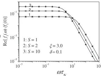
FIG. 5. The real parts of the normalized spectraf˜₁共␻兲/f₁共0兲vs

␻␶Nevaluated from the exact continued fraction solution关Eq.共17兲:

[image:8.612.90.256.541.666.2]

beingO共␧2_{兲and so on. Thus the Stratonovich representation} for spins关31兴, just as the well-known Wigner representation for particles关43兴, is well suited to the development of semi-classical methods of solution allowing one to obtain quantum corrections in a manner closely analogous to the classical case共see, e.g.,关5兴, Chap. 7兲.

Thus one may conclude for spins 共just as for particles兲 that the existing solution methods 共matrix continued frac-tions which can be evaluated by iterating a simple algorithm, integral representation of relaxation times, etc.兲 seamlessly carry over to the quantum case indeed suggesting new closed form quantum results via the corresponding classical ones; for example, the quantum integral relaxation time, Eq.共25兲

above. We have illustrated the phase-space method by con-sidering the simplest possible problem, namely, the longitu-dinal relaxation of an arbitrary spin in a uniform magnetic field of arbitrary strength directed along theZ axis 共the re-laxation of the transverse components of the magnetization can be treated in like manner using Eq. 共4兲 just as in the classical case关5兴兲. We remark that longitudinal relaxation in a uniform field is the simplest example of the phase method for spins as it is the rotational analog of the translational harmonic oscillator in the weak coupling limit considered by Agarwal关50兴 so that the quasiprobability density diffusion equation has the Fokker-Planck form for allS, hence pertur-bation theory is not required. This would not be true in gen-eral, e.g., for relaxation in nonaxially symmetric magneto-crystalline anisotropy and external field potentials, which invariably comprise two or more potential wells. Here per-turbation theory in the small parameter␧⬃S−1_{is required in} the evolution equation for the Wigner function共which unlike axially symmetric problems involves the conservative or Liouville term兲just as perturbation theory inប2is required in the corresponding quantum translational Brownian motion in an arbitrary potentialV共xˆ兲. Nevertheless our simple isotropic spin problem demonstrates clearly how one may calculate, using the phase-space method, the influence of spin size共in the weak bath spin coupling limit兲on the relaxation behav-ior.

ACKNOWLEDGMENT

This publication has emanated from research conducted with the financial support of Science Foundation Ireland 共Project No. 05/RFP/PHY/0070兲.

APPENDIX A: PHASE-SPACE DESCRIPTION OF SPIN SYSTEMS

To provide a phase-space description of spin systems, Stratonovich in 1956 关31兴 introduced the quasiprobability 共Wigner兲 distribution function on the sphere. Alternative quasiprobability distribution functions for spins have also been proposed and discussed, e.g., in Refs.关32–40兴using the spin coherent-state representation. Moreover, Várilly and Gracia-Bondía关33兴 have shown that the spin coherent-state approach is equivalent to the Stratonovich formalism 共see also关39,40兴兲. The Wigner quasiprobability distribution func-tion on the surface of the unit sphere for a spin system given

by Stratonovich关31兴is defined by the invertible map关39兴

W_␴共␽,␸,t兲= Tr兵␳ˆ wˆ_␴共␽,␸兲其, 共A1兲 where␴parametrizes quasiprobability functions of spins be-longing to the SU共2兲 dynamical symmetry group, ␳ˆ is the system density matrix, and wˆ_␴共␽,␸兲 is the Wigner-Stratonovich operator or kernel of the bijective transforma-tion given by Eq.共A1兲defined as

wˆ_␴共␽,␸兲=

冑

4␲ 2S+ 1

兺

_L=0

2S

兺

M=−L L

共C_S,S,L,0S,S 兲−␴Y_L,M* 共␽,␸兲Tˆ_L,M共S兲 , 共A2兲 such that Tr兵wˆ_␴共␽,␸兲其= 1 and 2S+1_4␲ 兰_␪,␸wˆ_␴共␽,␸兲sin␽d␽d␸

=Iˆ. HereIˆis the identity matrix,YL,M共␽,␸兲are the spherical harmonics关62兴, and the Tˆ_L,M共S兲 are the irreducible tensor共 po-larization兲operators with matrix elements given by关62兴

关Tˆ_L,M共S兲 兴m_⬘,m=

冑

2L+ 1 2S+ 1CS,m,L,M

S,m⬘

−S艋m,m

⬘

艋S−L⬍M⬍L, 0艋L艋2S, and C_S,S,L,0S,S and

C_S,m,L,MS,m⬘ are the Clebsch-Gordan coefficients 关62兴. The den-sity matrix ␳ˆ may then be expressed using the kernel Eq. 共A2兲as关39兴

␳ˆ=2S+ 1 4␲

冕

_␪,␸

wˆ_␴共␽,␸兲W−␴共␽,␸,t兲sin␽d␽d␸. 共A3兲 Knowledge of the functionW−␴共␽,␸,t兲 now allows one to calculate the average value of an arbitrary spin operatorAˆ

in the same way as the corresponding function for transla-tional motion关39兴because theW−␴_{共␽,␸,t兲provide the} over-lap relation

具Aˆ典= Tr兵␳ˆ Aˆ其=2S+ 1 4␲

冕

_␪,␸A

␴_{共␽,␸兲W}−␴_{共␽,␸,t兲sin␽d␽d␸,} 共A4兲

whereA␴共␽,␸兲 is the Weyl symbol of the operator Aˆ 共see, e.g.,关44兴兲defined as

A␴共␽,␸兲= Tr兵Aˆ wˆ_␴共␽,␸兲其. 共A5兲 As an example, we evaluate A␴共␽,␸兲 for the operator

SˆZ. Noting Eqs. 共A2兲 and 共A5兲 and known relations

SˆZ=

冑

S共S+ 1兲共2S+ 1兲/ 3Tˆ_1,0共 S_兲

and Tr兵Tˆ_L

1,M1

共S_兲

Tˆ_L

2,M2

共S_兲 其 =共−1兲M1␦

L₁,L2␦M1,−M2 关62兴, we obtain

SZ␴共␽,␸兲= Tr兵SˆZwˆ␴共␽,␸兲其

=共C_S,S,1,0S,S 兲−␴

冑

4␲S共S+ 1兲/3Y_1,0* 共␽,␸兲 =S共1−␴兲/2共S+ 1兲共1+␴兲/2cos␽.

In particular, for ␴= 1 we have SZ1共␽,␸兲=共S+ 1兲cos␽. Fur-thermore, at equilibrium, the phase-space distribution

␳ˆ_eq=e␤ប␻0SˆZ_/Z

S, 共A6兲 and vice versa. ForS= 1 / 2, this can readily be demonstrated by analytically substituting into Eqs.共A1兲–共A3兲and共A6兲the known representation of the matrix exponentiale␣SˆZ_{in terms}

of the irreducible tensor operatorsTˆ_L,M共S兲 共关62兴, Secs. 2.5 and 2.6兲, viz.,

e␣SˆZ₌

冑

₂关_Tˆ

0,0

共1/2兲_{cosh共␣/2兲+Tˆ}

1,0

共1/2兲_{sinh共␣/2兲兴.}

Thus one obtains after some algebra关cf. Eq.共5兲兴

W_eq−1共␽兲=

冋

cosh

冉

1

2␤ប␻0

冊

+ sinh

冉

1

2␤ប␻0

冊

cos␽

册

冒

Z1/2. In the present paper, we considerW−1_{共␽,t兲only关} correspond-ing to Eq.共4兲兴; thus we omit in all equations the superscript −1 inW−1共␽,t兲andW_eq−1共␽兲.

APPENDIX B: DERIVATION OFD„1…_„z_…ANDD„2…_„z_…

Knowing the functional form of the master equation共8兲

for the spin, the next crucial step is to determine the drift and diffusion coefficients D共1兲_{共z兲 and D}共2兲_{共z兲. Hitherto} calcula-tions ofD共1兲共z兲andD共2兲共z兲for a quantum spin subjected to a dc magnetic fieldH0 have been undertaken in Refs.关30,42兴 by starting from the master equation for the density matrix␳ˆ. Undoubtedly, many methods of determining these coeffi-cients exist. Among a wide variety of options for determin-ingD共1兲共z兲andD共2兲共z兲, we shall select here the extension to the semiclassical case of a simple heuristic idea originally used by Einstein, Smoluchowski, Langevin, and Kramers in order to calculate drift and diffusion coefficients in the clas-sical theory of the Brownian motion. Recently, we have ap-plied this approach for the quantum translational Brownian motion关46,48兴.

In order to determine the explicit form of D共1兲_{共z兲 and}

D共2兲_{共z兲 in Eq.共8兲, we first recall that the equilibrium} distri-butionWeq共z兲from Eq.共13兲must be the equilibrium solution of the generic master equation共8兲, i.e., it must satisfy

⳵

⳵z

冉

D

共2兲_共z兲⳵

⳵zWeq共z兲−D

共1兲_{共z兲Weq共z兲}

冊

_{= 0. 共B1兲} One may seek a solution forD共1兲共z兲 andD共2兲共z兲in the form

D共1兲_{共z兲=共1 −z}2_兲关a 0 S

+a₁Sz+a₂Sz2_{+ ¯兴, 共B2兲}

D共2兲共z兲=共1 −z2兲关b₀S+b₁Sz+b₂Sz2+ ¯兴. 共B3兲 By substituting Eqs.共B2兲 and共B3兲into Eq. 共B1兲, one then finds ifWeq共z兲 from Eq.共13兲is a solution of Eq. 共B1兲, that only the coefficients a₀S,b₀S, andb₁S are nonzero and D共1兲_共z兲 andD共2兲_{共z兲are given by}

D共1兲共z兲= 2Sb₀S共1 −z2兲tanh ␰ 2S

and

D共2兲共z兲=bS₀共1 −z2兲

冋

1 +ztanh ␰ 2S

册

.

In order to define the normalizing coefficientb₀Sone can use the fluctuation-dissipation theorem 关30兴 and the additional condition that in the classical limit 共␤→0, S→⬁, and ␤S

→const兲, the drift and diffusion coefficients D共1兲共z兲 and

D共2兲_{共z兲 must reduce to their classical counterparts for the} rotational Brownian motion of a classical spin关5,18,19,30兴

D共1兲共z兲→␰共1 −z2兲/2␶N andD共2兲共z兲→共1 −z2兲/2␶N, so thatb₀S=共e␰/S_{+ 1兲/共4␶N兲 andD}共1兲_共z兲andD共2兲_{共z兲are given} by Eqs. 共9兲 and 共10兲. In the derivation of D共1兲_{共z兲 and}

D共2兲_{共z兲we have imposed the stationary solution of the master} equation as the distributionWeq共z兲, Eq.共5兲, corresponding to the equilibrium density matrix␳ˆ_eqgiven by Eq.共A6兲, which describes the system in thermal equilibrium without coupling to the thermal bath. It is known from the theory of quantum open systems关63兴, that the equilibrium state, in general, may deviate from the canonical distribution ␳ˆ_eq; the latter de-scribes the thermal equilibrium of the system in the weak coupling and high temperature limits only. A detailed discus-sion of this problem is given, e.g., by Gevaet al. 关64兴. The imposition of the phase-space distributionWeq共z兲as the equi-librium solution of Eq.共B1兲so yieldingD共1兲共z兲 andD共2兲共z兲, appears to be the exact analog of theansatz used by Gross and Lebowitz 关65兴 in their formulation of quantum kinetic models of impulsive collisions. According to关65兴, for a sys-tem with a time dependent HamiltonianHˆ, the equation gov-erning the time behavior of the density matrix␳ˆ is Eq. 共3兲, where the collision kernel operatorQˆ satisfies the condition

Qˆ共␳ˆeq兲= 0. Equation共B1兲is entirely analogous to this condi-tion. The conditionQˆ共␳ˆeq兲= 0 has also been used by Redfield 关11兴 in the calculation of the matrix elements of the relax-ation operator Qˆ in the context of his theory of relaxation processes.

关1兴A. Abragam, The Principles of Nuclear Magnetism共Oxford University Press, London, 1961兲.

关2兴C. P. Slichter,Principles of Magnetic Resonance 共 Springer-Verlag, Berlin, 1990兲, and references therein.

关3兴D. Gatteschi, R. Sessoli, and J. Villain,Molecular Nanomag-nets共Oxford University Press, Oxford, 2006兲.

关4兴W. T. Coffey and P. C. Fannin, J. Phys.: Condens. Matter 14,

3677共2002兲.

关5兴W. T. Coffey, Yu. P. Kalmykov, and J. T. Waldron,The Lange-vin Equation, 2nd ed.共World Scientific, Singapore, 2004兲. 关6兴L. Néel, Ann. Geophys.共C.N.R.S.兲 5, 99共1949兲.

关7兴P. Debye,Polar Molecules共Chemical Catalog Co. New York, 1929; reprinted by Dover, New York, 1954兲.

关9兴N. Bloembergen, E. M. Purcell, and R. V. Pound, Phys. Rev. 73, 679共1948兲.

关10兴R. K. Wangsness and F. Bloch, Phys. Rev. 89, 728共1953兲. 关11兴A. G. Redfield, IBM J. Res. Dev. 1, 19共1957兲.

关12兴P. N. Argyres, P. L. Kelley, and G. Kelley, Phys. Rev. 134, A98共1964兲.

关13兴W. F. Brown, Jr., Phys. Rev. 130, 1677共1963兲. 关14兴W. F. Brown, Jr., IEEE Trans. Magn. 15, 1196共1979兲. 关15兴M. I. Shliomis and V. I. Stepanov, Adv. Chem. Phys. 87, 1

共1994兲.

关16兴L. Landau and E. Lifshitz, Phys. Z. Sowjetunion 8, 153 共1935兲.

关17兴T. L. Gilbert, Phys. Rev. 100, 1243共1955兲.

关18兴R. Kubo and N. Hashitsume, Suppl. Prog. Theor. Phys. 46, 210共1970兲.

关19兴A. Kawabata, Prog. Theor. Phys. 48, 2237共1972兲.

关20兴A. M. Jayannvar, Z. Phys. B: Condens. Matter82, 153共1991兲. 关21兴K. Miyazaki and K. Seki, J. Chem. Phys. 108, 7052共1998兲. 关22兴H. A. Kramers, Physica共Amsterdam兲 7, 284共1940兲. 关23兴D. A. Smith and F. A. de Rozario, J. Magn. Magn. Mater. 3,

219共1976兲.

关24兴W. T. Coffey, D. A. Garanin, and D. J. McCarthy, Adv. Chem. Phys. 117, 483共2001兲.

关25兴C. P. Bean and J. D. Livingston, J. Appl. Phys. 30, S120 共1959兲.

关26兴W. Wernsdorfer, Adv. Chem. Phys. 118, 99共2001兲. 关27兴H. Haken,Laser Theory共Springer, Berlin, 1984兲.

关28兴W. P. Schleich,Quantum Optics in Phase Space共Wiley-VCH, Berlin, 2001兲.

关29兴L. M. Narducci and C. M. Bowden, Phys. Rev. A 11, 280 共1975兲.

关30兴Y. Takahashi and F. Shibata, J. Phys. Soc. Jpn. 38, 656共1975兲; J. Stat. Phys. 14, 49共1976兲.

关31兴R. L. Stratonovich, Zh. Eksp. Teor. Fiz.31, 1012共1956兲 关Sov. Phys. JETP 4, 891共1957兲兴.

关32兴F. A. Berezin, Commun. Math. Phys. 40, 153共1975兲. 关33兴J. C. Várilly and J. M. Gracia-Bondía, Ann. Phys.共N.Y.兲 190,

107共1989兲.

关34兴M. O. Scully and K. Wodkiewicz, Found. Phys. 24, 85共1994兲. 关35兴J. M. Radcliffe, J. Phys. A 4, 313共1971兲.

关36兴F. T. Arecchi, E. Courtens, R. Gilmore, and H. Thomas, Phys. Rev. A 6, 2211共1972兲.

关37兴G. S. Agarwal, Phys. Rev. A 24, 2889共1981兲; 57, 671共1998兲; J. P. Dowling, G. S. Agarwal, and W. P. Schleich, ibid. 49, 4101共1994兲.

关38兴C. Brif and A. Mann, Phys. Rev. A 59, 971共1999兲. 关39兴A. B. Klimov, J. Math. Phys. 43, 2202共2002兲.

关40兴D. Zueco and I. Calvo, J. Phys. A: Math. Theor. 40, 4635 共2007兲.

关41兴N. Nashitsume, F. Shibata, and M. Shingu, J. Stat. Phys. 17,

155共1977兲; F. Shibata, Y. Takahashi, and N. Nashitsume,ibid.

17, 171共1977兲.

关42兴F. Shibata, J. Phys. Soc. Jpn. 49, 15共1980兲; F. Shibata and M. Asou,ibid. 49, 1234共1980兲; F. Shibata and C. Ushiyama,ibid.

62, 381共1993兲.

关43兴E. P. Wigner, Phys. Rev. 40, 749共1932兲.

关44兴S. R. de Groot and L. G. Suttorp,Foundations of Electrody-namics 共North-Holland, Amsterdam, 1972兲, Chaps. VI and VII.

关45兴J. L. García-Palacios, Europhys. Lett. 65, 735 共2004兲; J. L. García-Palacios and D. Zueco, J. Phys. A 37, 10735共2004兲. 关46兴W. T. Coffey, Yu. P. Kalmykov, S. V. Titov, and B. P.

Mulli-gan, Europhys. Lett. 77, 20011 共2007兲; J. Phys. A: Math. Theor. 40, F91共2007兲.

关47兴W. T. Coffey, Yu. P. Kalmykov, S. V. Titov, and B. P. Mulli-gan, Phys. Rev. E 75, 041117共2007兲; W. T. Coffey, Yu. P. Kalmykov, and S. V. Titov, J. Chem. Phys. 127, 074502 共2007兲.

关48兴W. T. Coffey, Yu. P. Kalmykov, S. V. Titov, and B. P. Mulli-gan, Phys. Chem. Chem. Phys. 9, 3361共2007兲.

关49兴H. Risken, The Fokker-Planck Equation, 2nd ed. 共 Springer-Verlag, Berlin, 1989兲.

关50兴G. S. Agarwal, Phys. Rev. A 4, 739共1971兲.

关51兴A. Morita, J. Phys. D 11, 1357共1978兲; 12, 991共1979兲. 关52兴J. T. Waldron, Yu. P. Kalmykov, and W. T. Coffey, Phys. Rev.

E 49, 3976共1994兲.

关53兴N. G. van Kampen, J. Stat. Phys. 80, 23共1995兲. 关54兴D. A. Garanin, Phys. Rev. E 54, 3250共1996兲. 关55兴D. A. Garanin, Phys. Rev. E 55, 2569共1997兲.

关56兴J. L. García-Palacios and D. Zueco, J. Phys. A 39, 13243 共2006兲; D. Zueco and J. L. García-Palacios, Phys. Rev. B 73, 104448共2006兲.

关57兴J. L. García-Palacios and S. Dattagupta, Phys. Rev. Lett. 95, 190401共2005兲.

关58兴A. Aharoni, Introduction to the Theory of Ferromagnetism

共Oxford University Press, Oxford, 2000兲.

关59兴Yu. P. Kalmykov, J. L. Déjardin, and W. T. Coffey, Phys. Rev. E 55, 2509共1997兲.

关60兴E. T. Whittaker and G. N. Watson,A Course of Modern Analy-sis, 4th ed.共Cambridge University Press, Cambridge, England, 1927兲.

关61兴R. Kubo, J. Phys. Soc. Jpn. 12, 570共1957兲.

关62兴D. A. Varshalovich, A. N. Moskalev, and V. K. Khersonskii,

Quantum Theory of Angular Momentum 共World Scientific, Singapore, 1998兲.

关63兴U. Weiss,Quantum Dissipative Systems, 2nd ed.共World Sci-entific, Singapore, 1999兲.

关64兴E. Geva, E. Rosenman, and D. Tannor, J. Chem. Phys. 113, 1380共2000兲.