A Latent Variable Model Approach to PMI-based Word Embeddings
Sanjeev Arora, Yuanzhi Li, Yingyu Liang, Tengyu Ma, Andrej Risteski Computer Science Department, Princeton University
35 Olden St, Princeton, NJ 08540
{arora,yuanzhil,yingyul,tengyu,risteski}@cs.princeton.edu
Abstract
Semantic word embeddings represent the meaning of a word via a vector, and are cre-ated by diverse methods. Many use non-linear operations on co-occurrence statistics, and have hand-tuned hyperparameters and reweighting methods.
This paper proposes a new generative model, a dynamic version of the log-linear topic model of Mnih and Hinton (2007). The method-ological novelty is to use the prior to com-pute closed form expressions for word statis-tics. This provides a theoretical justifica-tion for nonlinear models like PMI, word2vec, and GloVe, as well as some hyperparame-ter choices. It also helps explain why low-dimensional semantic embeddings contain lin-ear algebraic structure that allows solution of word analogies, as shown by Mikolov et al. (2013a) and many subsequent papers. Experimental support is provided for the gen-erative model assumptions, the most impor-tant of which is that latent word vectors are fairly uniformly dispersed in space.
1 Introduction
Vector representations of words (word embeddings) try to capture relationships between words as dis-tance or angle, and have many applications in com-putational linguistics and machine learning. They are constructed by various models whose unify-ing philosophy is that the meanunify-ing of a word is defined by “the company it keeps” (Firth, 1957), namely, co-occurrence statistics. The simplest
meth-ods use word vectors that explicitly represent co-occurrence statistics. Reweighting heuristics are known to improve these methods, as is dimension reduction (Deerwester et al., 1990). Some reweight-ing methods are nonlinear, which include takreweight-ing the square root of co-occurrence counts (Rohde et al., 2006), or the logarithm, or the related Pointwise Mu-tual Information (PMI) (Church and Hanks, 1990). These are collectively referred to as Vector Space Models, surveyed in (Turney and Pantel, 2010).
Neural network language models (Rumelhart et al., 1986; Rumelhart et al., 1988; Bengio et al., 2006; Collobert and Weston, 2008a) propose an-other way to construct embeddings: the word vec-tor is simply the neural network’s internal repre-sentation for the word. This method is nonlinear and nonconvex. It was popularized via word2vec, a family of energy-based models in (Mikolov et al., 2013b; Mikolov et al., 2013c), followed by a ma-trix factorization approach called GloVe (Penning-ton et al., 2014). The first paper also showed how to solve analogies using linear algebra on word em-beddings. Experiments and theory were used to sug-gest that these newer methods are related to the older PMI-based models, but with new hyperparameters and/or term reweighting methods (Levy and Gold-berg, 2014b).
But note that even the old PMI method is a bit mysterious. The simplest version considers a sym-metric matrix with each row/column indexed by a word. The entry for (w, w0) is PMI(w, w0) = logpp(w(w,w)p(w0)0), wherep(w, w0)is the empirical
prob-ability of wordsw, w0appearing within a window of certain size in the corpus, andp(w) is the marginal
385
probability ofw. (More complicated models could use asymmetric matrices with columns correspond-ing to context words or phrases, and also involve ten-sorization.) Then word vectors are obtained by low-rank SVD on this matrix, or a related matrix with term reweightings. In particular, the PMI matrix is found to be closely approximated by a low rank ma-trix: there exist word vectors in say300dimensions,
which is much smaller than the number of words in the dictionary, such that
hvw, vw0i ≈PMI(w, w0) (1.1)
where≈should be interpreted loosely.
There appears to be no theoretical explanation for this empirical finding about the approximate low rank of the PMI matrix. The current paper addresses this. Specifically, we propose a probabilistic model of text generation that augments the log-linear topic model of Mnih and Hinton (2007) with dynamics, in the form of a random walk over a latent discourse space. The chief methodological contribution is us-ing the model priors to analytically derive a closed-form expression that directly explains (1.1); see The-orem 2.2 in Section 2. Section 3 builds on this in-sight to give a rigorous justification for models such as word2vec and GloVe, including the hyperparam-eter choices for the latter. The insight also leads to a mathematical explanation for why these word em-beddings allow analogies to be solved using linear algebra; see Section 4. Section 5 shows good empir-ical fit to this model’s assumtions and predictions, including the surprising one that word vectors are pretty uniformly distributed (isotropic) in space. 1.1 Related work
Latent variable probabilistic models of language have been used for word embeddings before, includ-ing Latent Dirichlet Allocation (LDA) and its more complicated variants (see the survey (Blei, 2012)), and some neurally inspired nonlinear models (Mnih and Hinton, 2007; Maas et al., 2011). In fact, LDA evolved out of efforts in the 1990s to provide a gen-erative model that “explains” the success of older vector space methods like Latent Semantic Index-ing (Papadimitriou et al., 1998; Hofmann, 1999). However, none of these earlier generative models has been linked to PMI models.
Levy and Goldberg (2014b) tried to relate word2vec to PMI models. They showed that if there were no dimension constraint in word2vec, specifically, the “skip-gram with negative sampling (SGNS)” version of the model, then its solutions would satisfy (1.1), provided the right hand side were replaced by PMI(w, w0)−βfor some scalarβ. However, skip-gram is a discriminative model (due to the use of negative sampling), not generative. Fur-thermore, their argument only applies to very high-dimensional word embeddings, and thus does not address low-dimensional embeddings, which have superior quality in applications.
Hashimoto et al. (2016) focuses on issues simi-lar to our paper. They model text generation as a random walk on words, which are assumed to be embedded as vectors in a geometric space. Given that the last word produced wasw, the probability that the next word isw0 is assumed to be given by h(|vw −vw0|2) for a suitable function h, and this
model leads to an explanation of (1.1). By contrast our random walk involves a latent discourse vector, which has a clearer semantic interpretation and has proven useful in subsequent work, e.g. understand-ing structure of word embeddunderstand-ings for polysemous words Arora et al. (2016). Also our work clarifies some weighting and bias terms in the training objec-tives of previous methods (Section 3) and also the phenomenon discussed in the next paragraph.
Researchers have tried to understand why vec-tors obtained from the highly nonlinear word2vec models exhibit linear structures (Levy and Goldberg, 2014a; Pennington et al., 2014). Specifically, for analogies like “man:woman::king:??,” queen hap-pens to be the word whose vectorvqueenis the most similar to the vectorvking −vman+vwoman. This suggests that simple semantic relationships, such as
masculinevsfemininetested in the above example, correspond approximately to a single direction in space, a phenomenon we will henceforth refer to as
RELATIONS=LINES.
failure in analogy solving. In our explanation, the low dimensionality of the word vectors plays a key role. This can also be seen as a theoretical expla-nation of the old observation that dimension reduc-tion improves the quality of word embeddings for various tasks. The intuitive explanation often given —that smaller models generalize better—turns out to be fallacious, since the training method for cre-ating embeddings makes no reference to analogy solving. Thus there is no a priori reason why low-dimensional model parameters (i.e., lower model ca-pacity) should lead to better performance in anal-ogy solving, just as there is no reason they are bet-ter at some other unrelated task like predicting the weather.
1.2 Benefits of generative approaches
In addition to giving some form of “unification” of existing methods, our generative model also brings more intepretability to word embeddings beyond tra-ditional cosine similarity and even analogy solving. For example, it led to an understanding of how the different senses of a polysemous word (e.g., bank) reside in linear superposition within the word bedding (Arora et al., 2016). Such insight into em-beddings may prove useful in the numerous settings in NLP and neuroscience where they are used.
Another new explanatory feature of our model is that low dimensionality of word embeddings plays a key theoretical role —unlike in previous papers where the model is agnostic about the di-mension of the embeddings, and the superiority of low-dimensional embeddings is an empirical finding (starting with Deerwester et al. (1990)). Specifically, our theoretical analysis makes the key assumption that the set of all word vectors (which are latent vari-ables of the generative model) are spatially isotropic, which means that they have no preferred direction in space. Havingnvectors be isotropic ind dimen-sions requires d n. This isotropy is needed in the calculations (i.e., multidimensional integral) that yield (1.1). It also holds empirically for our word vectors, as shown in Section 5.
The isotropy of low-dimensional word vectors also plays a key role in our explanation of the
RELATIONS=LINES phenomenon (Section 4). The
isotropy has a “purification” effect that mitigates the effect of the (rather large) approximation error in the
PMI models.
2 Generative model and its properties The model treats corpus generation as a dynamic process, where the t-th word is produced at stept. The process is driven by the random walk of a dis-course vector ct ∈ <d. Its coordinates represent what is being talked about.1 Each word has a
(time-invariant) latent vectorvw ∈ <dthat captures its cor-relations with the discourse vector. We model this bias with a log-linear word production model:
Pr[wemitted at timet|ct]∝exp(hct, vwi). (2.1) The discourse vectorctdoes a slow random walk (meaning thatct+1 is obtained fromct by adding a small random displacement vector), so that nearby words are generated under similar discourses. We are interested in the probabilities that word pairs co-occur near each other, so occasional big jumps in the random walk are allowed because they have negligi-ble effect on these probabilities.
A similar log-linear model appears in Mnih and Hinton (2007) but without the random walk. The linear chain CRF of Collobert and Weston (2008b) is more general. The dynamic topic model of Blei and Lafferty (2006) utilizes topic dynamics, but with a linear word production model. Belanger and Kakade (2015) have proposed a dynamic model for text us-ing Kalman Filters, where the sequence of words is generated from Gaussian linear dynamical systems, rather than the log-linear model in our case.
The novelty here over such past works is a the-oretical analysis in the method-of-moments tradi-tion (Hsu et al., 2012; Cohen et al., 2012). Assuming a prior on the random walk we analytically integrate out the hidden random variables and compute a sim-ple closed form expression that approximately con-nects the model parameters to the observable joint probabilities (see Theorem 2.2). This is reminis-cent of analysis of similar random walk models in finance (Black and Scholes, 1973).
Model details. Letndenote the number of words andddenote the dimension of the discourse space, where1 ≤ d ≤ n. Inspecting (2.1) suggests word
vectors need to have varying lengths, to fit the empir-ical finding that word probabilities satisfy a power law. Furthermore, we will assume that in the bulk, the word vectors are distributed uniformly in space, earlier referred to as isotropy. This can be quantified as a prior in the Bayesian tradition. More precisely, the ensemble of word vectors consists of i.i.d draws generated byv = s·v, whereˆ vˆis from the
spher-ical Gaussian distribution, andsis a scalar random variable. We assumesis a random scalar with ex-pectationτ = Θ(1)andsis always upper bounded byκ, which is another constant. Hereτ governs the expected magnitude ofhv, cti, and it is particularly important to choose it to beΘ(1)so that the
distribu-tionPr[w|ct]∝exp(hvw, cti)is interesting.2 More-over, the dynamic range of word probabilities will roughly equalexp(κ2), so one should think ofκ as an absolute constant like5. These details aboutsare important for realistic modeling but not too impor-tant in our analysis. (Furthermore, readers uncom-fortable with this simplistic Bayesian prior should look at Section 2.1 below.)
Finally, we clarify the nature of the random walk. We assume that the stationary distribution of the ran-dom walk is uniform over the unit sphere, denoted byC. The transition kernel of the random walk can be in any form so long as at each step the movement of the discourse vector is at most2/
√
din`2norm.3 This is still fast enough to let the walk mix quickly in the space.
The following lemma (whose proof appears in the appendix) is central to the analysis. It says that un-der the Bayesian prior, the partition functionZc = P
wexp(hvw, ci), which is the implied normaliza-tion in equanormaliza-tion (2.1), is close to some constant Z for most of the discoursesc. This can be seen as a plausible theoretical explanation of a phenomenon called self-normalization in log-linear models: ig-noring the partition function or treating it as a con-stant (which greatly simplifies training) is known to often give good results. This has also been studied
2A largerτwill makePr[w
|ct]too peaked and a smaller one will make it too uniform.
3More precisely, the proof extends to any symmetric
prod-uct stationary distributionCwith sub-Gaussian coordinate sat-isfyingEc
kck2 = 1, and the steps are such that for allc
t, Ep(ct+1|ct)[exp(κ
√
dkct+1−ctk)] ≤ 1 +2for some small
2.
in (Andreas and Klein, 2014).
Lemma 2.1(Concentration of partition functions).
If the word vectors satisfy the Bayesian prior de-scribed in the model details, then
Pr
c∼C[(1−z)Z ≤Zc≤(1 +z)Z]≥1−δ, (2.2) forz=Oe(1/√n), andδ= exp(−Ω(log2n)).
The concentration of the partition functions then leads to our main theorem (the proof is in the ap-pendix). The theorem gives simple closed form approximations for p(w), the probability of word
w in the corpus, and p(w, w0), the probability
that two words w, w0 occur next to each other. The theorem states the result for the window size q = 2, but the same analysis works for pairs
that appear in a small window, say of size 10, as
stated in Corollary 2.3. Recall that PMI(w, w0) = log[p(w, w0)/(p(w)p(w0))].
Theorem 2.2. Suppose the word vectors satisfy the inequality(2.2), and window sizeq = 2. Then,
logp(w, w0) = kvw+vw0k
2 2
2d −2 logZ±, (2.3)
logp(w) = kvwk
2 2
2d −logZ±. (2.4)
for = O(z) +Oe(1/d) +O(2). Jointly these
imply:
PMI(w, w0) = hvw, vw0i
d ±O(). (2.5) Remarks 1. Since the word vectors have`2 norm of the order of √d, for two typical word vectors vw, vw0,kvw+vw0k22is of the order ofΘ(d).
There-fore the noise levelis very small compared to the leading term 1
2dkvw+vw0k22. For PMI however, the noise levelO()could be comparable to the leading
term, and empirically we also find higher error here. Remarks 2. Variants of the expression for joint probability in (2.3) had been hypothesized based upon empirical evidence in Mikolov et al. (2013b) and also Globerson et al. (2007), and Maron et al. (2010) .
Corollary 2.3. Letpq(w, w0)be the co-occurrence
probability in windows of sizeq, and PMIq(w, w0)
be the corresponding PMI value. Then
logpq(w, w0) = k
vw+vw0k22
2d −2 logZ+γ±,
PMIq(w, w0) = h
vw, vw0i
d +γ±O().
whereγ = logq(q2−1).
It is quite easy to see that Theorem 2.2 implies the Corollary 2.3, as when the window size is q the pairw, w0 could appear in any of q2positions within the window, and the joint probability ofw, w0 is roughly the same for any positions because the discourse vector changes slowly. (Of course, the er-ror term gets worse as we consider larger window sizes, although for any constant size, the statement of the theorem is correct.) This is also consistent with the shiftβ for fitting PMI in (Levy and Gold-berg, 2014b), which showed that without dimension constraints, the solution to skip-gram with negative sampling satisfies PMI(w, w0)−β =hvw, vw0ifor
a constantβthat is related to the negative sampling in the optimization. Our result justifies via a genera-tive model why this should be satisfied even for low dimensional word vectors.
2.1 Weakening the model assumptions
For readers uncomfortable with Bayesian priors, we can replace our assumptions with concrete proper-ties of word vectors that are empirically verifiable (Section 5.1) for our final word vectors, and in fact also for word vectors computed using other recent methods.
The word meanings are assumed to be represented by some “ground truth” vectors, which the experi-menter is trying to recover. These ground truth vec-tors are assumed to be spatially isotropic in the bulk, in the following two specific ways: (i) For almost all unit vectorscthe sum Pwexp(hvw, ci) is close to a constant Z; (ii) Singular values of the matrix of word vectors satisfy properties similar to those of random matrices, as formalized in the paragraph be-fore Theorem 4.1. Our Bayesian prior on the word vectors happens to imply that these two conditions hold with high probability. But the conditions may hold even if the prior doesn’t hold. Furthermore,
they are compatible with all sorts of local structure among word vectors such as existence of cluster-ings, which would be absent in truly random vectors drawn from our prior.
3 Training objective and relationship to other models
To get a training objective out of Theorem 2.2, we reason as follows. Let Xw,w0 be the number of
times words w and w0 co-occur within the same window in the corpus. The probabilityp(w, w0) of
such a co-occurrence at any particular time is given by (2.3). Successive samples from a random walk are not independent. But if the random walk mixes fairly quickly (the mixing time is related to the log-arithmof the vocabulary size), then the distribution ofXw,w0’s is very close to a multinomial
distribu-tionMul( ˜L,{p(w, w0)}), where L˜ = Pw,w0Xw,w0
is the total number of word pairs.
Assuming this approximation, we show below that the maximum likelihood values for the word vectors correspond to the following optimization,
min {vw},C
X
w,w0
Xw,w0
log(Xw,w0)− kvw+vw0k22−C
2
As is usual, empirical performance is improved by weighting down very frequent word pairs, possibly because very frequent words such as “the” do not fit our model. This is done by replacing the weighting Xw,w0 by its truncation min{Xw,w0, Xmax} where
Xmax is a constant such as100. We call this
objec-tive with the truncated weightsSN(SquaredNorm). We now give its derivation. Maximizing the like-lihood of{Xw,w0}is equivalent to maximizing
`= log
Y
(w,w0)
p(w, w0)Xw,w0
.
Denote the logarithm of the ratio between the ex-pected count and the empirical count as
∆w,w0 = log ˜
Lp(w, w0)
Xw,w0
!
. (3.1)
Xw,w0’s.
`=c+ X
(w,w0)
Xw,w0∆w,w0 (3.2)
On the other hand, usingex ≈1 +x+x2/2when xis small,4we have
˜
L= X
(w,w0)
˜
Lpw,w0 =
X
(w,w0)
Xw,w0e∆w,w0
≈ X
(w,w0)
Xw,w0 1 + ∆w,w0+ ∆2
w,w0 2
! .
Note thatL˜ =P
(w,w0)Xw,w0, so
X
(w,w0)
Xw,w0∆w,w0 ≈ −1 2
X
(w,w0)
Xw,w0∆2w,w0.
Plugging this into (3.2) leads to
2(c−`)≈ X
(w,w0)
Xw,w0∆2w,w0. (3.3)
So maximizing the likelihood is approximately equivalent to minimizing the right hand side, which (by examining (3.1)) leads to our objective.
Objective for training with PMI. A similar ob-jective PMI can be obtained from (2.5), by com-puting an approximate MLE, using the fact that the error between the empirical and true value of PMI(w, w0)is driven by the smaller termp(w, w0), and not the larger termsp(w), p(w0).
min {vw},C
X
w,w0
Xw,w0 PMI(w, w0)− hvw, vw0i2
This is of course very analogous to classical VSM methods, with a novel reweighting method.
Fitting to either of the objectives involves solving a version of Weighted SVD which is NP-hard, but empirically seems solvable in our setting via Ada-Grad (Duchi et al., 2011).
4This Taylor series approximation has an error of the order ofx3, but ignoring it can be theoretically justified as follows.
For a largeXw,w0, its value approaches its expectation and thus the corresponding∆w,w0is close to 0 and thus ignoring∆3w,w0 is well justified. The terms where∆w,w0 is significant corre-spond toXw,w0’s that are small. But empirically,Xw,w0’s obey a power law distribution (see, e.g. Pennington et al. (2014)) us-ing which it can be shown that these terms contribute a small fraction of the final objective (3.3). So we can safely ignore the errors. Full details appear in the ArXiv version of this pa-per (Arora et al., 2015).
Connection to GloVe. Compare SNwith the ob-jective used by GloVe (Pennington et al., 2014): X
w,w0
f(Xw,w0)(log(Xw,w0)−hvw, vw0i−sw−sw0−C)2
withf(Xw,w0) = min{Xw,w3/40,100}.Their
weight-ing methods and the need forbias termssw, sw0, C
were derived by trial and error; here they are all predicted and given meanings due to Theorem 2.2, specificallysw =kvwk2.
Connection to word2vec(CBOW). The CBOW model in word2vec posits that the probability of a word wk+1 as a function of the previous k words w1, w2, . . . , wk:
pwk+1
{wi}ki=1
∝exp(hvwk+1,
1
k k X
i=1 vwii).
This expression seems mysterious since it de-pends upon the average word vector for the previ-ousk words. We show it can be theoretically jus-tified. Assume a simplified version of our model, where a small window of k words is generated as follows: samplec∼ C, whereCis a uniformly ran-dom unit vector, then sample (w1, w2, . . . , wk) ∼
exp(hPki=1vwi, ci)/Zc. Furthermore, assumeZc=
Zfor anyc.
Lemma 3.1. In the simplified version of our model, the Maximum-a-Posteriori (MAP) estimate of c
given(w1, w2, . . . , wk)is Pk
i=1vwi
kPki=1vwik2.
Proof. The c maximizing p(c|w1, w2, . . . , wk) is the maximizer of p(c)p(w1, w2, . . . , wk|c). Since p(c) = p(c0) for any c, c0, and we have p(w1, w2, . . . , wk|c) = exp(hPivwi, ci)/Z, the
maximizer is clearlyc=
Pk i=1vwi
kPki=1vwik2.
Thus using the MAP estimate of ct gives essen-tially the same expression as CBOW apart from the rescaling, which is often omitted due to computa-tional efficiency in empirical works.
4 ExplainingRELATIONS=LINES
As mentioned, word analogies like “a:b::c:??” can be solved via a linear algebraic expression:
argmin
d k
where vectors have been normalized such that
kvdk2 = 1. This suggests that the semantic rela-tionships being tested in the analogy are character-ized by a straight line,5referred to earlier asRELA
-TIONS=LINES.
Using our model we will show the following for low-dimensional embeddings: for each such relation Rthere is a directionµRin space such that for any word paira, bsatisfying the relation,va−vbis like µR plus some noise vector. This happens for rela-tions satisfying a certain condition described below. Empirical results supporting this theory appear in Section 5, where this linear structure is further lever-aged to slightly improve analogy solving.
A side product of our argument will be a mathematical explanation of the empirically well-established superiority of low-dimensional word embeddings over high-dimensional ones in this set-ting (Levy and Goldberg, 2014a). As mentioned ear-lier, the usual explanation that smaller models gen-eralize better is fallacious.
We first sketch what was missing in prior attempts to prove versions of RELATIONS=LINES from first
principles. The basic issue is approximation er-ror: the difference between the best solution and the 2nd best solution to (4.1) is typically small, whereas the approximation error in the objective in the low-dimensional solutions is larger. For instance, if one uses ourPMIobjective, then the weighted average of the termwise error in (2.5) is17%, and the
expres-sion in (4.1) above contains six inner products. Thus in principle the approximation error could lead to a failure of the method and the emergence of linear relationship, but it does not.
Prior explanations. Pennington et al. (2014) try to propose a model where such linear relationships should occurby design. They posit thatqueen is a solution to the analogy “man:woman::king:??”
be-5Note that this interpretation has been disputed; e.g., it is argued in Levy and Goldberg (2014a) that (4.1) can be under-stood using only the classical connection between inner product and word similarity, using which the objective (4.1) is slightly improved to a different objective called 3COSMUL. However, this “explanation” is still dogged by the issue of large termwise error pinpointed here, since inner product is only a rough ap-proximation to word similarity. Furthermore, the experiments
in Section 5 clearly support theRELATIONS=LINES
interpreta-tion.
cause
p(χ|king)
p(χ|queen) ≈
p(χ|man)
p(χ|woman), (4.2)
where p(χ | king) denotes the conditional
proba-bility of seeing word χ in a small window of text around king. Relationship (4.2) is intuitive since both sides will be ≈ 1 for gender-neutral χ like “walks” or “food”, will be> 1when χis like “he,
Henry” and will be< 1whenχis like “dress, she,
Elizabeth.” This was also observed by Levy and Goldberg (2014a). Given (4.2), they then posit that the correct model describing word embeddings in terms of word occurrences must be ahomomorphism
from(<d,+)to(<+,×), so vector differences map
to ratios of probabilities. This leads to the expres-sion
pw,w0 =hvw, vw0i+bw+bw0,
and their method is a (weighted) least squares fit for this expression. One shortcoming of this argument is that the homomorphism assumptionassumesthe linear relationships instead of explaining them from a more basic principle. More importantly, the empir-ical fit to the homomorphism has nontrivial approx-imation error, high enough that it does not imply the desired strong linear relationships.
Levy and Goldberg (2014b) show that empiri-cally, skip-gram vectors satisfy
hvw, vw0i ≈PMI(w, w0) (4.3)
up to some shift. They also give an argument sug-gesting this relationship must be present if the so-lution is allowed to be very high-dimensional. Un-fortunately, that argument does not extend to low-dimensional embeddings. Even if it did, the issue of termwise approximation error remains.
This argument will assume the analogy in ques-tion involves a relaques-tion that obeys Pennington et al.’s suggestion in (4.2). Namely, for such a relation R there exists functionνR(·)depending only upon R such that for anya, b satisfying R there is a noise
functionξa,b,R(·)for which: p(χ|a)
p(χ|b) =νR(χ)·ξa,b,R(χ) (4.4)
For different wordsχthere is huge variation in (4.4), so the multiplicative noise may be large.
Our goal is to show that the low-dimensional word embeddings have the property that there is a vectorµR such that for every pair of wordsa, bin that relation, va−vb = µR +noise vector, where the noise vector is small.
Taking logarithms of (4.4) results in:
log
p(χ|a)
p(χ|b)
= log(νR(χ)) +ζa,b,R(χ) (4.5) Theorem 2.2 implies that the left-hand side sim-plifies to logpp((χχ||ab)) = 1dhvχ, va−vbi +a,b(χ)
wherecaptures the small approximation errors in-duced by the inexactness of Theorem 2.2. This adds yet more noise! Denoting by V the n×dmatrix whose rows are thevχvectors, we rewrite (4.5) as:
V(va−vb) =dlog(νR) +ζa,b,R0 (4.6) wherelog(νR)in the element-wise log of vectorνR andζa,b,R0 =d(ζa,b,R−a,b,R)is the noise.
In essence, (4.6) shows thatva−vbis a solution to a linear regression indvariables andmconstraints, withζa,b,R0 being the “noise.” Thedesign matrixin the regression isV, the matrix of all word vectors, which in our model (as well as empirically) satisfies an isotropy condition. This makes it random-like, and thus solving the regression by left-multiplying byV†, the pseudo-inverse ofV, ought to “denoise” effectively. We now show that it does.
Our model assumed the set of all word vectors satisfies bulk properties similar to a set of Gaus-sian vectors. The next theorem will only need the following weaker properties. (1) The smallest non-zero singular value ofV is larger than some constant c1 times the quadratic mean of the singular values, namely,kVkF/
√
d. Empirically we findc1 ≈ 1/3
holds; see Section 5. (2) The left singular vectors behave like random vectors with respect to ζa,b,R0 , namely, have inner product at mostc2kζa,b,R0 k/
√
n withζa,b,R0 , for some constantc2. (3) The max norm of a row inV isO(√d). The proof is included in the
appendix.
Theorem 4.1(Noise reduction). Under the condi-tions of the previous paragraph, the noise in the dimension-reduced semantic vector space satisfies
kζ¯a,b,Rk2.kζa,b,R0 k2
√
d n .
As a corollary, the relative error in the dimension-reduced space is a factor ofpd/nsmaller.
5 Experimental verification
In this section, we provide experiments empirically supporting our generative model.
Corpus. All word embedding vectors are trained on the English Wikipedia (March 2015 dump). It is pre-processed by standard approach (removing non-textual elements, sentence splitting, and tokeniza-tion), leaving about 3 billion tokens. Words that
appeared less than1000times in the corpus are ig-nored, resulting in a vocabulary of68,430. The
co-occurrence is then computed using windows of 10 tokens to each side of the focus word.
Training method. Our embedding vectors are trained by optimizing theSNobjective using Ada-Grad (Duchi et al., 2011) with initial learning rate of
0.05and 100 iterations. ThePMIobjective derived
from (2.5) was also used.SNhas average (weighted) term-wise error of5%, andPMIhas17%. We
ob-served that SN vectors typically fit the model bet-ter and have betbet-ter performance, which can be ex-plained by larger errors in PMI, as implied by Theo-rem 2.2. So, we only report the results forSN.
For comparison, GloVe and two variants of word2vec (skip-gram and CBOW) vectors are trained. GloVe’s vectors are trained on the same co-occurrence asSNwith the default parameter values.6
word2vec vectors are trained using a window size of 10, with other parameters set to default values.7
0.5 1 1.5 2 0
20 40
Partition function value
Percentage
(a) SN
0.5 1 1.5 2
0 20 40 60 80 100
Partition function value
(b) GloVe
0.5 1 1.5 2
0 20 40 60 80
Partition function value
(c) CBOW
0.5 1 1.5 2
0 20 40
Partition function value
[image:9.612.127.488.50.138.2](d) skip-gram
Figure 1: The partition functionZc. The figure shows the histogram ofZcfor1000random vectorscof appropriate
norm, as defined in the text. The x-axis is normalized by the mean of the values. The values Zc for different c
concentrate around the mean, mostly in[0.9,1.1]. This concentration phenomenon is predicted by our analysis.
6 8 10 12 14 16 18
1 2 3 4 5 6 7 8 9 10
Natural logarithm of frequency
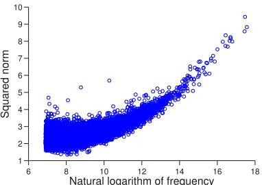
[image:9.612.91.282.199.334.2]Squared norm
Figure 2: The linear relationship between the squared norms of our word vectors and the logarithms of the word frequencies. Each dot in the plot corresponds to a word, where x-axis is the natural logarithm of the word fre-quency, andy-axis is the squared norm of the word vec-tor. The Pearson correlation coefficient between the two is 0.75, indicating a significant linear relationship, which strongly supports our mathematical prediction, that is, equation (2.4) of Theorem 2.2.
5.1 Model verification
Experiments were run to test our modeling assump-tions. First, we tested two counter-intuitive proper-ties: the concentration of the partition function Zc for different discourse vectorsc(see Theorem 2.1), and the random-like behavior of the matrix of word embeddings in terms of its singular values (see The-orem 4.1). For comparison we also tested these properties for word2vec and GloVe vectors, though they are trained by different objectives. Finally, we tested the linear relation between the squared norms of our word vectors and the logarithm of the word frequencies, as implied by Theorem 2.2.
Partition function. Our theory predicts the counter-intuitive concentration of the partition func-tionZc =Pw0exp(c>vw0)for a random discourse
vectorc (see Lemma 2.1). This is verified empiri-cally by picking a uniformly random direction, of normkck= 4/µw, whereµwis the average norm of the word vectors.8 Figure 1(a) shows the histogram
of Zc for 1000 such randomly chosen c’s for our
vectors. The values are concentrated, mostly in the range [0.9,1.1] times the mean. Concentration is
also observed for other types of vectors, especially for GloVe and CBOW.
Isotropy with respect to singular values. Our theoretical explanation of RELATIONS=LINES
as-sumes that the matrix of word vectors behaves like a random matrix with respect to the properties of singular values. In our embeddings, the quadratic mean of the singular values is 34.3, while the min-imum non-zero singular value of our word vectors is 11. Therefore, the ratio between them is a small constant, consistent with our model. The ratios for GloVe, CBOW, and skip-gram are 1.4, 10.1, and 3.1, respectively, which are also small constants.
Squared norms v.s. word frequencies. Figure 2 shows a scatter plot for the squared norms of our vectors and the logarithms of the word frequencies. A linear relationship is observed (Pearson correla-tion 0.75), thus supporting Theorem 2.2. The cor-relation is stronger for high frequency words, pos-sibly because the corresponding terms have higher weights in the training objective.
This correlation is much weaker for other types
8Note that our model uses the inner products between the
discourse vectors and word vectors, so it is invariant if the dis-course vectors are scaled byswhile the word vectors are scaled by1/sfor anys >0. Therefore, one needs to choose the norm
ofcproperly. We assumekckµw =
√
d/κ≈4for a constant
κ= 5so that it gives a reasonable fit to the predicted dynamic
Relations SN GloVe CBOW skip-gram
G semanticsyntactic 0.840.61 0.850.65 0.790.71 0.730.68
total 0.71 0.73 0.74 0.70
M
adjective 0.50 0.56 0.58 0.58
noun 0.69 0.70 0.56 0.58
verb 0.48 0.53 0.64 0.56
[image:10.612.84.286.53.138.2]total 0.53 0.57 0.62 0.57
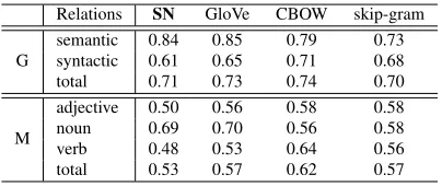
Table 1: The accuracy on two word analogy task testbeds: G (the GOOGLE testbed); M (the MSR testbed). Per-formance is close to the state of the art despite using a generative model with provable properties.
of word embeddings. This is possibly because they have more free parameters (“knobs to turn”), which imbue the embeddings with other properties. This can also cause the difference in the concentration of the partition function for the two methods.
5.2 Performance on analogy tasks
We compare the performance of our word vec-tors on analogy tasks, specifically the two testbeds GOOGLE and MSR (Mikolov et al., 2013a; Mikolov et al., 2013c). The for-mer contains 7874 semantic questions such as
“man:woman::king:??”, and 10167 syntactic ones
such as “run:runs::walk:??.” The latter has 8000
syntactic questions for adjectives, nouns, and verbs. To solve these tasks, we use linear algebraic queries.9 That is, first normalize the vectors to unit
norm and then solve “a:b::c:??” by
argmin
d k
va−vb−vc+vdk22. (5.1) The algorithm succeeds if the bestdhappens to be correct.
The performance of different methods is pre-sented in Table 1. Our vectors achieve performance comparable to the state of art on semantic analogies (similar accuracy as GloVe, better than word2vec). On syntactic tasks, they achieve accuracy0.04lower
than GloVe and skip-gram, while CBOW typically outperforms the others.10 The reason is probably
9One can instead use the 3COSMUL in (Levy and Goldberg,
2014a), which increases the accuracy by about3%. But it is not linear while our focus here is the linear algebraic structure.
10It was earlier reported that skip-gram outperforms
CBOW (Mikolov et al., 2013a; Pennington et al., 2014). This may be due to the different training data sets and hyperparame-ters used.
relation cap-com cap-wor adj-adv opp
1st 0.65±0.07 0.61±0.09 0.35±0.17 0.42±0.16 2nd 0.02±0.28 0.00±0.23 0.07±0.24 0.01±0.25
Table 2: The verification of relation directions on 2 se-mantic and 2 syntactic relations in the GOOGLE testbed. Relations include cap-com: capital-common-countries; cap-wor: capital-world; adj-adv: gram1-adjective-to-adverb; opp: gram2-opposite. For each relation, take vab = va −vb for pairs(a, b)in the relation, and then
calculate the top singular vectors of the matrix formed by thesevab’s. The row with label “1st”/“2nd” shows the
co-sine similarities of individualvabto the 1st/2nd singular
vector (the mean and standard deviation).
that our model ignores local word order, whereas the other models capture it to some extent. For ex-ample, a word “she” can affect the context by a lot and determine if the next word is “thinks” rather than “think”. Incorporating such linguistic features in the model is left for future work.
5.3 VerifyingRELATIONS=LINES
The theory in Section 4 predicts the existence of a direction for a relation, whereas earlier Levy and Goldberg (2014a) had questioned if this phe-nomenon is real. The experiment uses the analogy testbed, where each relation is tested using 20 or
[image:10.612.308.548.54.87.2]SN GloVe CBOW skip-gram
w/oRD 0.71 0.73 0.74 0.70
RD(k= 20) 0.74 0.77 0.79 0.75
RD(k= 30) 0.79 0.80 0.82 0.80
[image:11.612.88.279.52.106.2]RD(k= 40) 0.76 0.80 0.80 0.77
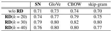
Table 3: The accuracy of the RD algorithm (i.e., the cheater method) on the GOOGLE testbed. The RD al-gorithm is described in the text. For comparison, the row “w/oRD” shows the accuracy of the old method without usingRD.
Cheating solver for analogy testbeds. The above linear structure suggests a better (but cheating) way to solve the analogy task. This uses the fact that the same semantic relationship (e.g., masculine-feminine, singular-plural) is tested many times in the testbed. If a relationRis represented by a direction µRthen the cheating algorithm can learn this direc-tion (via rank 1 SVD) after seeing a few examples of the relationship. Then use the following method of solving “a:b::c:??”: look for a worddsuch that vc−vdhas the largest projection onµR, the relation direction for(a, b). This can boost success rates by
about10%.
The testbed can try to combat such cheating by giving analogy questions in a random order. But the cheating algorithm can justclusterthe presented analogies to learn which of them are in the same relation. Thus the final algorithm, named analogy solver with relation direction (RD), is: take all vec-torsva−vb for all the word pairs (a, b) presented among the analogy questions and dok-means clus-tering on them; for each (a, b), estimate the
rela-tion direcrela-tion by taking the first singular vector of its cluster, and substitute that forva−vbin (5.1) when solving the analogy. Table 3 shows the performance on GOOGLE with different values ofk; e.g. using ourSNvectors andk = 30 leads to0.79accuracy.
Thus future designers of analogy testbeds should re-member not to test the same relationship too many times! This still leaves other ways to cheat, such as learning the directions for interesting semantic rela-tions from other collecrela-tions of analogies.
Non-cheating solver for analogy testbeds. Now we show that even if a relationship is tested only once in the testbed, there is a way to use the above structure. Given “a:b::c:??,” the solver first finds the top 300 nearest neighbors of a and those of
SN GloVe CBOW skip-gram
w/oRD-nn 0.71 0.73 0.74 0.70
RD-nn(k= 10) 0.71 0.74 0.77 0.73
RD-nn(k= 20) 0.72 0.75 0.77 0.74
[image:11.612.322.527.52.106.2]RD-nn(k= 30) 0.73 0.76 0.78 0.74
Table 4: The accuracy of theRD-nn algorithm on the GOOGLE testbed. The algorithm is described in the text. For comparison, the row “w/oRD-nn” shows the accu-racy of the old method without usingRD-nn.
b, and then finds among these neighbors the top k pairs(a0, b0)so that the cosine similarities between
va0 −vb0 andva−vb are largest. Finally, the solver uses these pairs to estimate the relation direction (via rank 1 SVD), and substitute this (corrected) estimate forva−vbin (5.1) when solving the analogy. This al-gorithm is named analogy solver with relation direc-tion by nearest neighbors (RD-nn). Table 4 shows its performance, which consistently improves over the old method by about3%.
6 Conclusions
A simple generative model has been introduced to explain the classical PMI based word embedding models, as well as recent variants involving energy-based models and matrix factorization. The model yields an optimization objective with essentially “no knobs to turn”, yet the embeddings lead to good per-formance on analogy tasks, and fit other predictions of our generative model. A model with fewer knobs to turn should be seen as a better scientific explana-tion (Occam’s razor), and certainly makes the em-beddings more interpretable.
The spatial isotropy of word vectors is both an assumption in our model, and also a new empir-ical finding of our paper. We feel it may help with further development of language models. It is important for explaining the success of solv-ing analogies via low dimensional vectors (RELA
-TIONS=LINES). It also implies that semantic
rela-tionships among words manifest themselves as spe-cial directions among word embeddings (Section 4), which lead to a cheater algorithm for solving anal-ogy testbeds.
unim-portant. Designing similar generative models (with provable and interpretable properties) with linguistic features is left for future work.
Acknowledgements
We thank the editors of TACL for granting a special relaxation of the page limit for our paper. We thank Yann LeCun, Christopher D. Manning, and Sham Kakade for helpful discussions at various stages of this work.
This work was supported in part by NSF grants CCF-1527371, DMS-1317308, Simons Investiga-tor Award, Simons Collaboration Grant, and ONR-N00014-16-1-2329. Tengyu Ma was supported in addition by Simons Award in Theoretical Computer Science and IBM PhD Fellowship.
References
Jacob Andreas and Dan Klein. 2014. When and why are log-linear models self-normalizing? InProceedings of the Annual Meeting of the North American Chapter of the Association for Computational Linguistics. Sanjeev Arora, Yuanzhi Li, Yingyu Liang, Tengyu Ma,
and Andrej Risteski. 2015. A latent variable model approach to PMI-based word embeddings. Technical report, ArXiV.http://arxiv.org/abs/1502.03520. Sanjeev Arora, Yuanzhi Li, Yingyu Liang, Tengyu
Ma, and Andrej Risteski. 2016. Linear al-gebraic structure of word senses, with applica-tions to polysemy. Technical report, ArXiV. http://arxiv.org/abs/1502.03520.
David Belanger and Sham M. Kakade. 2015. A linear dynamical system model for text. InProceedings of the 32nd International Conference on Machine Learn-ing.
Yoshua Bengio, Holger Schwenk, Jean-S´ebastien Sen´ecal, Fr´ederic Morin, and Jean-Luc Gauvain. 2006. Neural probabilistic language models. In Innovations in Machine Learning.
Fischer Black and Myron Scholes. 1973. The pricing of options and corporate liabilities. Journal of Political Economy.
David M. Blei and John D. Lafferty. 2006. Dynamic topic models. InProceedings of the 23rd International Conference on Machine Learning.
David M. Blei. 2012. Probabilistic topic models. Com-munication of the Association for Computing Machin-ery.
Kenneth Ward Church and Patrick Hanks. 1990. Word association norms, mutual information, and lexicogra-phy. Computational linguistics.
Shay B. Cohen, Karl Stratos, Michael Collins, Dean P. Foster, and Lyle Ungar. 2012. Spectral learning of latent-variable PCFGs. In Proceedings of the 50th Annual Meeting of the Association for Computational Linguistics: Long Papers-Volume 1.
Ronan Collobert and Jason Weston. 2008a. A uni-fied architecture for natural language processing: Deep neural networks with multitask learning. In Proceed-ings of the 25th International Conference on Machine Learning.
Ronan Collobert and Jason Weston. 2008b. A uni-fied architecture for natural language processing: Deep neural networks with multitask learning. In Proceed-ings of the 25th International Conference on Machine Learning.
Scott C. Deerwester, Susan T Dumais, Thomas K. Lan-dauer, George W. Furnas, and Richard A. Harshman. 1990. Indexing by latent semantic analysis. Journal of the American Society for Information Science. John Duchi, Elad Hazan, and Yoram Singer. 2011.
Adaptive subgradient methods for online learning and stochastic optimization. The Journal of Machine Learning Research.
John Rupert Firth. 1957.A synopsis of linguistic theory. Amir Globerson, Gal Chechik, Fernando Pereira, and Naftali Tishby. 2007. Euclidean embedding of co-occurrence data. Journal of Machine Learning Re-search.
Tatsunori B. Hashimoto, David Alvarez-Melis, and Tommi S. Jaakkola. 2016. Word embeddings as met-ric recovery in semantic spaces. Transactions of the Association for Computational Linguistics.
Thomas Hofmann. 1999. Probabilistic latent semantic analysis. InProceedings of the Fifteenth Conference on Uncertainty in Artificial Intelligence.
Daniel Hsu, Sham M. Kakade, and Tong Zhang. 2012. A spectral algorithm for learning hidden markov models. Journal of Computer and System Sciences.
Omer Levy and Yoav Goldberg. 2014a. Linguistic regu-larities in sparse and explicit word representations. In Proceedings of the Eighteenth Conference on Compu-tational Natural Language Learning.
Omer Levy and Yoav Goldberg. 2014b. Neural word em-bedding as implicit matrix factorization. InAdvances in Neural Information Processing Systems.
Yariv Maron, Michael Lamar, and Elie Bienenstock. 2010. Sphere embedding: An application to part-of-speech induction. InAdvances in Neural Information Processing Systems.
Tomas Mikolov, Kai Chen, Greg Corrado, and Jeffrey Dean. 2013a. Efficient estimation of word representa-tions in vector space. Proceedings of the International Conference on Learning Representations.
Tomas Mikolov, Ilya Sutskever, Kai Chen, Greg S. Cor-rado, and Jeff Dean. 2013b. Distributed represen-tations of words and phrases and their composition-ality. In Advances in Neural Information Processing Systems.
Tomas Mikolov, Wen-tau Yih, and Geoffrey Zweig. 2013c. Linguistic regularities in continuous space word representations. InProceedings of the Confer-ence of the North American Chapter of the Associa-tion for ComputaAssocia-tional Linguistics: Human Language Technologies.
Andriy Mnih and Geoffrey Hinton. 2007. Three new graphical models for statistical language modelling. In Proceedings of the 24th International Conference on Machine Learning.
Christos H. Papadimitriou, Hisao Tamaki, Prabhakar Raghavan, and Santosh Vempala. 1998. Latent se-mantic indexing: A probabilistic analysis. In Proceed-ings of the 7th ACM SIGACT-SIGMOD-SIGART Sym-posium on Principles of Database Systems.
Jeffrey Pennington, Richard Socher, and Christopher D. Manning. 2014. Glove: Global vectors for word rep-resentation. Proceedings of the Empiricial Methods in Natural Language Processing.
Douglas L. T. Rohde, Laura M. Gonnerman, and David C. Plaut. 2006. An improved model of seman-tic similarity based on lexical co-occurence. Commu-nication of the Association for Computing Machinery. David E. Rumelhart, Geoffrey E. Hinton, and James L. McClelland, editors. 1986. Parallel Distributed Pro-cessing: Explorations in the Microstructure of Cogni-tion.
David E. Rumelhart, Geoffrey E. Hinton, and Ronald J. Williams. 1988. Learning representations by back-propagating errors.Cognitive modeling.
Peter D. Turney and Patrick Pantel. 2010. From fre-quency to meaning: Vector space models of semantics. Journal of Artificial Intelligence Research.
A Proof sketches
Here we provide the proof sketches, while the com-plete proof can be found in the full version (Arora et al., 2015).
Proof sketch of Theorem 2.2 Letwandw0be two arbitrary words. Letcandc0denote two consecutive context vectors, wherec ∼ C andc0|cis defined by the Markov kernelp(c0 |c).
We start by using the law of total expectation, in-tegrating out the hidden variablescandc0:
p(w, w0) = E
c,c0
Pr[w, w0|c, c0]
= E
c,c0[p(w|c)p(w 0|c0)]
= E
c,c0
exp(hvw, ci) Zc
exp(hvw0, c0i)
Zc0
(A.1) An expectation like (A.1) would normally be dif-ficult to analyze because of the partition functions. However, we can assume the inequality (2.2), that is, the partition function typically does not vary much for most of context vectorsc. LetF be the event that bothc andc0 are within(1±z)Z. Then by (2.2) and the union bound, eventF happens with proba-bility at least1−2 exp(−Ω(log2n)). We will split
the right-hand side (RHS) of (A.1) into the parts ac-cording to whetherFhappens or not.
RHS of (A.1)= E
c,c0
exp(hvw, ci) Zc
exp(hvw0, c0i)
Zc0 1F
| {z }
T1
+ E
c,c0
exp(hvw, ci)
Zc
exp(hvw0, c0i)
Zc0 1F¯
| {z }
T2
(A.2) where F¯ denotes the complement of event F and 1F and1F¯ denote indicator functions forF andF¯, respectively. WhenF happens, we can replaceZc byZwith a1±z factor loss: The first term of the RHS of (A.2) equals to
T1 =
1±O(z)
Z2 E
c,c0
exp(hvw, ci) exp(hvw0, c0i)1F (A.3) On the other hand, we can useE[1F¯] = Pr[ ¯F]≤
exp(−Ω(log2n)) to show that the second term of
RHS of (A.2) is negligible,
This claim must be handled somewhat carefully since the RHS does not depend ondat all. Briefly, the reason this holds is as follows: in the regime when dis small (√d = o(log2n)), any word vec-torvw and discoursecsatisfies thatexp(hvw, ci) ≤
exp(kvwk) = exp(O(
√
d)), and since E[1F¯] =
exp(−Ω(log2n)), the claim follows directly; In the regime when d is large (√d = Ω(log2n)),
we can use concentration inequalities to show that except with a small probability exp(−Ω(d)) = exp(−Ω(log2n)), a uniform sample from the sphere
behaves equivalently to sampling all of the coor-dinates from a standard Gaussian distribution with mean 0 and variance 1
d, in which case the claim is not too difficult to show using Gaussian tail bounds. Therefore it suffices to only consider (A.3). Our model assumptions state thatcandc0 cannot be too different. We leverage that by rewriting (A.3) a little, and get that it equals
T1 =
1±O(z) Z2 Ec
"
exp(hvw, ci) E c0|c
exp(hvw0, c0i)
#
= 1±O(z)
Z2 Ec[exp(hvw, ci)A(c)] (A.5) whereA(c) := E
c0|c
exp(hvw0, c0i). We claim that
A(c) = (1±O(2)) exp(hvw0, ci). Doing some
al-gebraic manipulations, A(c) = exp(hvw0, ci) E
c0|c
exp(hvw0, c0−ci).
Furthermore, by our model assumptions,kc−c0k ≤ 2/
√
d. So
hvw, c−c0i ≤ kvwkkc−c0k=O(2)
and thusA(c) = (1±O(2)) exp(hvw0, ci).
Plug-ging the simplification ofA(c)to (A.5),
T1=
1±O(z)
Z2 E[exp(hvw+vw0, ci)]. (A.6) Since c has uniform distribution over the sphere, the random variable hvw+vw0, ci has distribution
pretty similar to Gaussian distributionN(0,kvw+ vw0k2/d), especially whendis relatively large.
Ob-serve thatE[exp(X)]has a closed form for Gaussian
random variableX ∼ N(0, σ2),
E[exp(X)] =
Z
x
1
σ√2π exp(− x2
2σ2) exp(x)dx
= exp(σ2/2). (A.7)
Bounding the difference between hvw+vw0, ci
from Gaussian random variable, we can show that for=Oe(1/d),
E[exp(hvw+vw0, ci)] = (1±) exp
kvw+vw0k2
2d
.
(A.8) Therefore, the series of simplifica-tion/approximation above (concretely, combining equations (A.1), (A.2), (A.4), (A.6), and (A.8)) lead to the desired bound on logp(w, w0) for the
case when the window sizeq = 2. The bound on
logp(w)can be shown similarly.
Proof sketch of Lemma 2.1 Note that for fixedc, when word vectors have Gaussian priors assumed as in our model, Zc = Pwexp(hvw, ci) is a sum of independent random variables.
We first claim that using proper concentration of measure tools, it can be shown that the vari-ance of Zc are relatively small compared to its mean Evw[Zc], and thus Zc concentrates around
its mean. Note this is quite non-trivial: the ran-dom variable exp(hvw, ci) is neither bounded nor subgaussian/sub-exponential, since the tail is ap-proximately inverse poly-logarithmic instead of in-verse exponential. In fact, the same concentration phenomenon does not happen for w. The occur-rence probability of wordwis not necessarily con-centrated because the`2norm ofvwcan vary a lot in our model, which allows the frequency of the words to have a large dynamic range.
So now it suffices to show thatEvw[Zc]for
differ-entcare close to each other. Using the fact that the word vector directions have a Gaussian distribution, Evw[Zc]turns out to only depend on the norm of c
(which is equal to 1). More precisely, E
vw
vectors. We sketch the proof of this. In our model, vw = sw·vˆw, wherevˆw is a Gaussian vector with identity covarianceI. Then
E vw
[Zc] =nE vw
[exp(hvw, ci)]
=nE
sw
" E vw|sw
[exp(hvw, ci)|sw]
#
where the second line is just an application of the law of total expectation, if we pick the norm of the (random) vector vw first, followed by its direction. Conditioned on sw, hvw, ci is a Gaussian random variable with variance kck2
2s2w, and therefore using similar calculation as in (A.7), we have
E vw|sw
[exp(hvw, ci)|sw] = exp(s2kck22/2).
Hence,Evw[Zc] =nEs[exp(s2kck22/2)]as needed. Proof of Theorem 4.1 The proof uses the standard analysis of linear regression. LetV =PΣQT be the SVD ofV and letσ1, . . . , σdbe the left singular val-ues ofV (the diagonal entries ofΣ). For notational
ease we omit the subscripts inζ¯andζ0since they are
not relevant for this proof. Since V† = QΣ−1PT and thusζ¯=V†ζ0 =QΣ−1PTζ0, we have
kζ¯k2≤σd−1kPTζ0k2. (A.10) We claim
σ−d1 ≤ r
1
c1n
. (A.11)
Indeed, Pd
i=1σ2i = O(nd), since the average squared norm of a word vector isd. The claim then follows from the first assumption. Furthermore, by the second assumption,kPTζ0k∞≤ √c2
nkζ0k2, so
kPTζ0k22 ≤ c22d
n kζ
0k2
2. (A.12) Plugging (A.11) and (A.12) into (A.10), we get
kζ¯k2 ≤
r
1
c1n
r c2
2d n kζ0k
2 2=
c2
√
d
√c
1nk ζ0k2