Functional Distributional Semantics
Guy Emerson and Ann Copestake Computer Laboratory
University of Cambridge {gete2,aac10}@cam.ac.uk
Abstract
Vector space models have become popu-lar in distributional semantics, despite the challenges they face in capturing various semantic phenomena. We propose a novel probabilistic framework which draws on both formal semantics and recent advances in machine learning. In particular, we sep-arate predicates from the entities they refer to, allowing us to perform Bayesian infer-ence based on logical forms. We describe an implementation of this framework us-ing a combination of Restricted Boltz-mann Machines and feedforward neural networks. Finally, we demonstrate the fea-sibility of this approach by training it on a parsed corpus and evaluating it on estab-lished similarity datasets.
1 Introduction
Current approaches to distributional semantics generally involve representing words as points in a high-dimensional vector space. However, vec-tors do not provide ‘natural’ composition oper-ations that have clear analogues with operoper-ations in formal semantics, which makes it challenging to perform inference, or capture various aspects of meaning studied by semanticists. This is true whether the vectors are constructed using acount approach (e.g. Turney and Pantel, 2010) or an em-beddingapproach (e.g. Mikolov et al., 2013), and indeed Levy and Goldberg (2014b) showed that there are close links between them. Even the ten-sorial approach described by Coecke et al. (2010) and Baroni et al. (2014), which naturally captures argument structure, does not allow an obvious ac-count of context dependence, or logical inference. In this paper, we build on insights drawn from formal semantics, and seek to learn
representa-tions which have a more natural logical structure, and which can be more easily integrated with other sources of information.
Our contributions in this paper are to introduce a novel framework for distributional semantics, and to describe an implementation and training regime in this framework. We present some initial results to demonstrate that training this model is feasible.
2 Formal Framework of Functional Distributional Semantics
In this section, we describe our framework, ex-plaining the connections to formal semantics, and defining our probabilistic model. We first motivate representing predicates with functions, and then explain how these functions can be incorporated into a representation for a full utterance.
2.1 Semantic Functions
We begin by assuming an extensional model struc-ture, as standard in formal semantics (Kamp and Reyle, 1993; Cann, 1993; Allan, 2001). In the simplest case, a model contains a set of entities, which predicates can be true or false of. Mod-els can be endowed with additional structure, such as for plurals (Link, 2002), although we will not discuss such details here. For now, the important point is that we should separate the representation of a predicate from the representations of the enti-ties it is true of.
We generalise this formalisation of predicates by treating truth values as random variables,1 1The move to replace absolute truth values with probabil-ities has parallels in much computational work based on for-mal logic. For example, Garrette et al. (2011) incorporate dis-tributional information in a Markov Logic Network (Richard-son and Domingos, 2006). However, while their approach allows probabilistic inference, they rely on existing distribu-tional vectors, and convert similarity scores to weighted logi-cal formulae. Instead, we aim to learn representations which are directly interpretable within in a probabilistic logic.
0 1
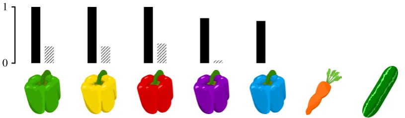
Figure 1: Comparison between asemantic functionand adistributionover a space of entities. The veg-etables depicted above (five differently coloured bell peppers, a carrot, and a cucumber) form a discrete semantic spaceX. We are interested in the truthtof the predicate forbell pepperfor an entityx∈ X. Solid bars: the semantic functionP(t|x)represents how much each entity is considered to be a pepper, and is bounded between0and1; it is high for all the peppers, but slightly lower for atypical colours. Shaded bars: the distributionP(x|t)represents our belief about an entity if all we know is that the pred-icate forbell pepperapplies to it; the probability mass must sum to1, so it is split between the peppers, skewed towards typical colours, and excluding colours believed to be impossible.
which enables us to apply Bayesian inference. For any entity, we can ask which predicates are true of it (or ‘applicable’ to it). More formally, if we take entities to lie in some semantic spaceX (whose di-mensions may denote different features), then we can take the meaning of a predicate to be a func-tion fromX to values in the interval[0,1], denot-ing how likely a speaker is to judge the predicate applicable to the entity. This judgement is variable between speakers (Labov, 1973), and for border-line cases, it is even variable for one speaker at dif-ferent times (McCloskey and Glucksberg, 1978).
Representing predicates as functions allows us to naturally capture vagueness (a predicate can be equally applicable to multiple points), and using values between 0 and 1 allows us to naturally cap-ture gradedness (a predicate can be more applica-ble to some points than to others). To use Labov’s example, the predicate forcupis equally applica-ble to vessels of different shapes and materials, but becomes steadily less applicable to wider vessels. We can also view such a function as a classifier – for example, the semantic function for the pred-icate for catwould be a classifier separating cats from non-cats. This ties in with a view of concepts as abilities, as proposed in both philosophy (Dum-mett, 1978; Kenny, 2010), and cognitive science (Murphy, 2002; Bennett and Hacker, 2008). A similar approach is taken by Larsson (2013), who argues in favour of representing perceptual con-cepts as classifiers of perceptual input.
Note that these functions do not directly de-fine probability distributions over entities. Rather, they define binary-valued conditional
distribu-tions,given an entity. We can write this asP(t|x), where x is an entity, and t is a stochastic truth value. It is only possible to get a correspond-ing distribution over entities given a truth value, P(x|t), if we have some background distribution P(x). If we do, we can apply Bayes’ Rule to get P(x|t)∝P(t|x)P(x). In other words, the truth of an expression depends crucially on our knowl-edge of the situation. This fits neatly within a ver-ificationist view of truth, as proposed by Dummett (1976), who argues that to understand a sentence is to know how we could verify or falsify it.
By using bothP(t|x)andP(x|t), we can distin-guish between underspecification and uncertainty as two kinds of ‘vagueness’. In the first case, we want to state partial information about an entity, but leave other features unspecified; P(t|x) rep-resents which kinds of entity could be described by the predicate, regardless of how likely we think the entities are. In the second case, we have uncer-tain knowledge about the entity;P(x|t)represents which kinds of entity we think are likely for this predicate, given all our world knowledge.
For example, bell peppers come in many colours, most typically green, yellow, orange or red. As all these colours are typical, the semantic function for the predicate for bell pepper would take a high value for each. In contrast, to define a probability distribution over entities, we must split probability mass between different colours,2
and for a large number of colours, we would only have a small probability for each. As purple and blue are atypical colours for a pepper, a speaker might be less willing to label such a vegetable a pepper, but not completely unwilling to do so – this linguistic knowledge belongs to the semantic function for the predicate. In contrast, after ob-serving a large number of peppers, we might con-clude that blue peppers do not exist, purple pers are rare, green peppers common, and red pep-pers more common still – this world knowledge belongs to the probability distribution over enti-ties. The contrast between these two quantities is depicted in figure 1, for a simple discrete space.
2.2 Incorporation with Dependency Minimal Recursion Semantics
Semantic dependency graphs have become popu-lar in NLP. We use Dependency Minimal Recur-sion Semantics (DMRS) (Copestake et al., 2005; Copestake, 2009), which represents meaning as a directed acyclic graph: nodes represent predi-cates/entities (relying on a one-to-one correspon-dence between them) and links (edges) repre-sent argument structure and scopal constraints. Note that we assume a neo-Davidsonian approach (Davidson, 1967; Parsons, 1990), where events are also treated as entities, which allows a better ac-count of adverbials, among other phenomena.
For example (simplifying a little), to represent “the dog barked”, we have three nodes, for the predicates the, dog, and bark, and two links: an
ARG1 link from bark to dog, and a RSTR link
from the todog. Unlike syntactic dependencies, DMRS abstracts over semantically equivalent ex-pressions, such as “dogs chase cats” and “cats are chased by dogs”. Furthermore, unlike other types of semantic dependencies, including Ab-stract Meaning Representations (Banarescu et al., 2012), and Prague Dependencies (B¨ohmov´a et al., 2003), DMRS is interconvertible with MRS, which can be given a direct logical interpretation.
We deal here with the extensional fragment of language, and while we can account for different quantifiers in our framework, we do not have space to discuss this here – for the rest of this paper, we neglect quantifiers, and the reader may assume that all variables are existentially quantified.
We can use the structure of a DMRS graph to define a probabilistic graphical model. This gives us a distribution over lexicalisations of the graph –
y z
x ARG1 ARG2
∈ X
tc, x tc, y tc, z
[image:3.595.308.524.60.167.2]∈ {⊥,>} |V|
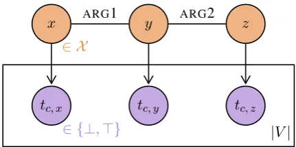
Figure 2: A situation composed of three entities. Top row: the entitiesx,y, andzlie in a semantic space X, jointly distributed according to DMRS links. Bottom row: each predicatecin the vocab-ularyV has a stochastic truth value for each entity.
given an abstract graph structure, where links are labelled but nodes are not, we have a process to generate a predicate for each node. Although this process is different for each graph structure, we can share parameters between them (e.g. accord-ing to the labels on links). Furthermore, if we have a distribution over graph structures, we can incor-porate that in our generative process, to produce a distribution over lexicalised graphs.
The entity nodes can be viewed as together rep-resenting a situation, in the sense of Barwise and Perry (1983). We want to be able to represent the entities without reference to the predicates – intu-itively, the world is the same however we choose to describe it. To avoid postulating causal struc-ture amongst the entities (which would be difficult for a large graph), we can model the entity nodes as an undirected graphical model, with edges ac-cording to the DMRS links. The edges are undi-rected in the sense that they don’t impose condi-tional dependencies. However, this is still compat-ible with having ‘directed’ semantic dependencies – the probability distributions are not symmetric, which maintains the asymmetry of DMRS links.
Each node takes values in the semantic spaceX, and the network defines a joint distribution over entities, which represents our knowledge about which situations are likely or unlikely. An exam-ple is shown in the top row of figure 2, of an entity y along with its two arguments x and z – these might represent an event, along with the agent and patient involved in the event. The structure of the graph means that we can factorise the joint distri-bution P(x, y, z) over the entities as being pro-portional to the productP(x, y)P(y, z).
y z
x ARG1 ARG2
∈ X
tc, x tc, y tc, z
∈ {⊥,>} |V|
p q r
[image:4.595.74.287.61.216.2]∈V
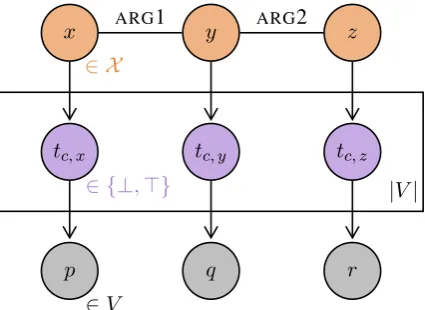
Figure 3: The probabilistic model in figure 2, ex-tended to generate utterances. Each predicate in the bottom row is chosen out of all predicates which are true for the corresponding entity.
node for every predicate in the vocabulary, where the value of the node is either true (>) or false (⊥). Each of these predicate nodes has a sin-gle directed link from the entity node, with the probability of the node being true being deter-mined by the predicate’s semantic function, i.e. P(tc, x=>|x) =tc(x). This is shown in the sec-ond row of figure 2, where the plate denotes that these nodes are repeated for each predicatecin the vocabularyV. For example, if the situation repre-sented a dog chasing a cat, then nodes liketdog, x, tanimal, x, andtpursue, y would be true (with high probability), whiletdemocracy, xortdog, zwould be false (with high probability).
The probabilistic model described above closely matches traditional model-theoretic semantics. However, while we could stop our semantic description there, we do not generally observe truth-value judgements for all predicates at once;3 rather, we observe utterances, which
have specific predicates. We can therefore define a final node for each entity, which takes values over predicates in the vocabulary, and which is conditionally dependent on the truth values of all predicates. This is shown in the bottom row of figure 3. Including these final nodes means that we can train such a model on observed utterances. The process of choosing a predicate from the true ones may be complex, potentially depending on speaker intention and other pragmatic factors – but in section 3, we will simply choose a true predicate at random (weighted by frequency).
3This corresponds to what Copestake and Herbelot (2012) call anideal distribution. If we have access to such informa-tion, we only need the two rows given in figure 2.
The separation of entities and predicates allows us to naturally capture context-dependent mean-ings. Following the terminology of Quine (1960), we can distinguish context-independent standing meaning from context-dependentoccasion mean-ing. Each predicate type has a corresponding semantic function – this represents its standing meaning. Meanwhile, each predicate token has a corresponding entity, for which there is a posterior distribution over the semantic space, conditioning on the rest of the graph and any pragmatic factors – this represents its occasion meaning.
Unlike previous approaches to context depen-dence, such as Dinu et al. (2012), Erk and Pad´o (2008), and Thater et al. (2011), we represent meanings in and out of context by different kinds of object, reflecting a type/token distinction. Even Herbelot (2015), who explicitly contrasts individ-uals and kinds, embeds both in the same space.
As an example of how this separation of pred-icates and entities can be helpful, suppose we would like “dogs chase cats” and “cats chase mice”to be true in a model, but“dogs chase mice” and“cats chase cats”to be false. In other words, there is a dependence between the verb’s argu-ments. If we represent each predicate by a single vector, it is not clear how to capture this. However, by separating predicates from entities, we can have two different entities whichchaseis true of, where one co-occurs with a dog-entity ARG1 and
cat-entityARG2, while the other co-occurs with a
cat-entityARG1 and a mouse-entityARG2. 3 Implementation
In the previous section, we described a general framework for probabilistic semantics. Here we give details of one way that such a framework can be implemented for distributional semantics, keeping the architecture as simple as possible. 3.1 Network Architecture
We take the semantic spaceX to be a set of binary-valued vectors,4 {0,1}N. A situation s is then composed of entity vectors x(1),· · ·, x(K)∈ X (where the number of entitiesKmay vary), along with links between the entities. We denote a link from x(n) to x(m) with labell as: x(n)−→l x(m). We define the background distribution over sit-uations using a Restricted Boltzmann Machine
(RBM) (Smolensky, 1986; Hinton et al., 2006), but rather than having connections between hidden and visible units, we have connections between components of entities, according to the links.
The probability of the network being in the particular configuration s depends on theenergy of the configuration, Eb(s), as shown in equa-tions (1)-(2). A high energy denotes an unlikely configuration. The energy depends on the edges of the graphical model, plus bias terms, as shown in (3). Note that we follow the Einstein sum-mation convention, where repeated indices indi-cate summation; although this notation is not typ-ical in NLP, we find it much clearer than matrix-vector notation, particularly for higher-order ten-sors. Each link labellhas a corresponding weight matrixW(l), which determines the strength of as-sociation between components of the linked enti-ties. The first term in (3) sums these contributions over all links x(n)−→l x(m) between entities. We also introduce bias terms, to control how likely an entity vector is, independent of links. The second term in (3) sums the biases over all entitiesx(n).
P(s) = Z1 exp−Eb(s) (1)
Z=X
s0
exp−Eb(s0) (2)
−Eb(s) = X
x(n)−→l x(m)
Wij(l)xi(n)x(jm)−X
x(n)
bix(in) (3)
Furthermore, since sparse representations have been shown to be beneficial in NLP, both for ap-plications and for interpretability of features (Mur-phy et al., 2012; Faruqui et al., 2015), we can en-force sparsity in these entity vectors by fixing a specific number of units to be active at any time. Swersky et al. (2012) introduce this RBM variant as the Cardinality RBM, and also give an efficient exact sampling procedure using belief propaga-tion. Since we are using sparse representations, we also assume that all link weights are non-negative. Now that we’ve defined the background distri-bution over situations, we turn to the semantic functionstc, which map entitiesxto probabilities. We implement these as feedforward networks, as shown in (4)-(5). For simplicity, we do not in-troduce any hidden layers. Each predicate c has a vector of weights W0(c), which determines the strength of association with each dimension of the semantic space, as well as a bias termb0(c). These
together define the energyEp(x, c)of an entityx with the predicate, which is passed through a sig-moid function to give a value in the range[0,1].
tc(x) =σ(−Ep(x, c)) = 1 + exp (1 Ep) (4)
−Ep(x, c) =Wi0(c)xi−b0(c) (5) Given the semantic functions, choosing a predi-cate for a entity can be hard-coded, for simplicity. The probability of choosing a predicate c for an entity xis weighted by the predicate’s frequency fc and the value of its semantic function tc(x)
(how true the predicate is of the entity), as shown in (6)-(7). This is a mean field approximation to the stochastic truth values shown in figure 3.
P(c|x) = 1
Zxfctc(x) (6) Zx=X
c0
fc0tc0(x) (7)
3.2 Learning Algorithm
To train this model, we aim to maximise the likeli-hood of observing the training data – in Bayesian terminology, this ismaximum a posteriori estima-tion. As described in section 2.2, each data point is a lexicalised DMRS graph, while our model de-fines distributions over lexicalisations of graphs. In other words, we take as given the observed distribution over abstract graph structures (where links are given, but nodes are unlabelled), and try to optimise how the model generates predicates (via the parametersWij(l), bi, Wi0(c), b0(c)).
For the family of optimisation algorithms based on gradient descent, we need to know the gradient of the likelihood with respect to the model param-eters, which is given in (8), wherex∈ Xis a latent entity, andc∈ V is an observed predicate (corre-sponding to the top and bottom rows of figure 3). Note that we extend the definition of energy from situations to entities in the obvious way: half the energy of an entity’s links, plus its bias energy. A full derivation of (8) is given in the appendix.
∂
∂θlogP(c) =Ex|c
∂ ∂θ
−Eb(x)
−Ex
∂ ∂θ
−Eb(x)
+Ex|c
(1−tc(x))∂θ∂ (−Ep(x, c))
−Ex|c
Ec0|x
(1−tc0(x)) ∂
∂θ −Ep(x, c0)
There are four terms in this gradient: the first two are for the background distribution, and the last two are for the semantic functions. In both cases, one term is positive, and conditioned on the data, while the other term is negative, and repre-sents the predictions of the model.
Calculating the expectations exactly is infeasi-ble, as this requires summing over all possible configurations. Instead, we can use a Markov Chain Monte Carlo method, as typically done for Latent Dirichlet Allocation (Blei et al., 2003; Grif-fiths and Steyvers, 2004). Our aim is to sample values of x and c, and use these samples to ap-proximate the expectations: rather than summing over all values, we just consider the samples. For each token in the training data, we introduce a la-tent entity vector, which we use to approximate the first, third, and fourth terms in (8). Additionally, we introduce a latent predicate for each latent en-tity, which we use to approximate the fourth term – this latent predicate is analogous to the negative samples used by Mikolov et al. (2013).
When resampling a latent entity conditioned on the data, the conditional distributionP(x|c)is un-known, and calculating it directly requires sum-ming over the whole semantic space. For this rea-son, we cannot apply Gibbs sampling (as used in LDA), which relies on knowing the conditional distribution. However, if we compare two enti-ties x andx0, the normalisation constant cancels
out in the ratio P(x0|c)/P(x|c), so we can use
the Metropolis-Hastings algorithm (Metropolis et al., 1953; Hastings, 1970). Given the current sam-plex, we can uniformly choose one unit to switch on, and one to switch off, to get a proposalx0. If
the ratio of probabilities shown in (9) is above 1, we switch the sample tox0; if it’s below 1, it is the
probability of switching tox0.
P(x0|c)
P(x|c) =
exp −Eb(x0) 1
Zx0tc(x0) exp (−Eb(x)) 1
Zxtc(x) (9)
Although Metropolis-Hastings avoids the need to calculate the normalisation constant Z of the background distribution, we still have the nor-malisation constant Zx of choosing a predicate given an entity. This constant represents the num-ber of predicates true of the entity (weighted by frequency). The intuitive explanation is that we should sample an entity which few predicates are true of, rather than an entity which many predi-cates are true of. We approximate this constant
by assuming that we have an independent contri-bution from each dimension ofx. We first aver-age over all predicates (weighted by frequency), to get the average predicateWavg. We then take the exponential of Wavg for the dimensions that we are proposing switching off and on – intuitively, if many predicates have a large weight for a given dimension, then many predicates will be true of an entity where that dimension is active. This is shown in (10), wherexandx0differ in dimensions
iandi0only, and wherekis a constant.
Zx
Zx0 ≈exp k W
avg
i −Wiavg0
(10)
We must also resample latent predicates given a latent entity, for the fourth term in (8). This can similarly be done using the Metropolis-Hastings algorithm, according to the ratio shown in (11).
P(c0|x)
P(c|x) =
fc0tc0(x)
fctc(x) (11) Finally, we need to resample entities from the background distribution, for the second term in (8). Rather than recalculating the samples from scratch after each weight update, we used fantasy particles (persistent Markov chains), which Tiele-man (2008) found effective for training RBMs. Resampling a particle can be done more straight-forwardly than resampling the latent entities – we can sample each entity conditioned on the other entities in the situation, which can be done exactly using belief propagation (see Yedidia et al. (2003) and references therein), as Swersky et al. (2012) applied to the Cardinality RBM.
To make weight updates from the gradients, we used AdaGrad (Duchi et al., 2011), with exponen-tial decay of the sum of squared gradients. We also used L1 and L2 regularisation, which determines our prior over model parameters.
as follows: we consider a situation with just one entity, and for each predicate, we find the mean-field entity vector given the pre-trained predicate parameters; we then fix all entity vectors in our training corpus to be these mean-field vectors, and find the positive pointwise mutual information of each each pair of entity dimensions, for each link label. In particular, we initialised predicate pa-rameters using our sparse SVO Word2Vec vectors, which we describe in section 4.2.
4 Training and Initial Experiments In this section, we report the first experiments car-ried out within our framework.
4.1 Training Data
Training our model requires a corpus of DMRS graphs. In particular, we used WikiWoods, an automatically parsed version of the July 2008 dump of the full English Wikipedia, distributed by DELPH-IN5. This resource was produced by
Flickinger et al. (2010), using the English Re-source Grammar (ERG; Flickinger, 2000), trained on the manually treebanked subcorpus WeScience (Ytrestøl et al., 2009), and implemented with the PET parser (Callmeier, 2001; Toutanova et al., 2005). To preprocess the corpus, we used the python packages pydelphin6 (developed by
Michael Goodman), and pydmrs7 (Copestake et
al., 2016).
For simplicity, we restricted attention to subject-verb-object (SVO) triples, although we should stress that this is not an inherent limita-tion of our model, which could be applied to ar-bitrary graphs. We searched for all verbs in the WikiWoods treebank, excluding modals, that had either anARG1 or anARG2, or both. We kept all
instances whose arguments were nominal, exclud-ing pronouns and proper nouns. The ERG does not automatically convert out-of-vocabulary items from their surface form to lemmatised predicates, so we applied WordNet’s morphological processor Morphy (Fellbaum, 1998), as available in NLTK (Bird et al., 2009). Finally, we filtered out situa-tions including rare predicates, so that every pred-icate appears at least five times in the dataset.
As a result of this process, all data was of the form (verb, ARG1, ARG2), where one (but not
5http://moin.delph-in.net/WikiWoods 6https://github.com/delph-in/pydelphin 7https://github.com/delph-in/pydmrs
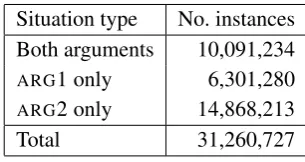
both) of the arguments may be missing. A sum-mary is given in table 1. In total, the dataset con-tains 72m tokens, with 88,526 distinct predicates.
Situation type No. instances Both arguments 10,091,234
ARG1 only 6,301,280 ARG2 only 14,868,213
[image:7.595.337.490.111.192.2]Total 31,260,727 Table 1: Size of the training data.
4.2 Evaluation
As our first attempt at evaluation, we chose to look at two lexical similarity datasets. The aim of this evaluation was simply to verify that the model was learning something reasonable. We did not expect this task to illustrate our model’s strengths, since we need richer tasks to exploit its full expressive-ness. Both of our chosen datasets aim to evalu-ate similarity, rather than thematic relevalu-atedness: the first is Hill et al. (2015)’s SimLex-999 dataset, and the second is Finkelstein et al. (2001)’s WordSim-353 dataset, which was split by Agirre et al. (2009) into similarity and relatedness subsets. So far, we have not tuned hyperparameters.
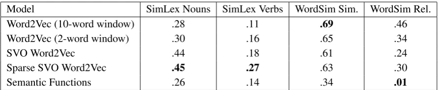
Results are given in table 2. We also trained Mikolov et al. (2013)’s Word2Vec model on the SVO data described in section 4.1, in order to give a direct comparison of models on the same training data. In particular, we used the continu-ous bag-of-words model with negative sampling, as implemented in ˇReh˚uˇrek and Sojka (2010)’s gensim package, with off-the-shelf hyperparame-ter settings. We also converted these to sparse vec-tors using Faruqui et al. (2015)’s algorithm, again using off-the-shelf hyperparameter settings. To measure similarity of our semantic functions, we treated each function’s parameters as a vector and used cosine similarity, for simplicity.
Model SimLex Nouns SimLex Verbs WordSim Sim. WordSim Rel.
Word2Vec (10-word window) .28 .11 .69 .46
Word2Vec (2-word window) .30 .16 .65 .34
SVO Word2Vec .44 .18 .61 .24
Sparse SVO Word2Vec .45 .27 .63 .30
Semantic Functions .26 .14 .34 .01
Table 2: Spearman rank correlation of different models with average annotator judgements. Note that we would like to have alowscore on the final column (which measures relatedness, rather than similarity).
[image:8.595.76.524.61.153.2]flood/water(related verb and noun) .06 flood/water(related nouns) .43 law/lawyer(related nouns) .44 sadness/joy(near-antonyms) .77 happiness/joy(near-synonyms) .78 aunt/uncle(differ in a single feature) .90 cat/dog(differ in many features) .92
Table 3: Similarity scores for thematically related words, and various types of co-hyponym.
et al. reported (even when we used less preprocess-ing or a different edition of Wikipedia), although still worse than our sparse SVO Word2Vec model. It is interesting to note that training Word2Vec on verbs and their arguments gives noticeably bet-ter results on SimLex-999 than training on full sentences, even though far less data is being used:
∼72m tokens, rather than ∼1000m. The better performance suggests that semantic dependencies may provide more informative contexts than sim-ple word windows. This is in line with previous results, such as Levy and Goldberg (2014a)’s work on using syntactic dependencies. Nonetheless, this result deserves further investigation.
Of all the models we tested, only our semantic function model failed on the relatedness subset of WordSim-353. We take this as a positive result, since it means the model clearly distinguishes re-latedness and similarity.
Examples of thematically related predicates and various kinds of co-hyponym are given in table 3, along with our model’s similarity scores. How-ever, it is not clear that it is possible, or even de-sirable, to represent these varied relationships on a single scale of similarity. For example, it could be sensible to treatauntanduncleeither as synonyms (they refer to relatives of the same degree of re-latedness) or as antonyms (they are “opposite” in some sense). Which view is more appropriate will depend on the application, or on the context.
Nouns and verbs are very strongly distin-guished, which we would expect given the struc-ture of our model. This can be seen in the simi-larity scores betweenfloodandwater, whenflood is considered either as a verb or as a noun.8
SimLex-999 generally assigns low scores to near-antonyms, and to pairs differing in a single fea-ture, which might explain why the performance of our model is not higher on this task. However, the separation of thematically related predicates from co-hyponyms is a promising result.
5 Related Work
As mentioned above, Coecke et al. (2010) and Ba-roni et al. (2014) introduce a tensor-based frame-work that incorporates argument structure through tensor contraction. However, for logical inference, we need to know how one vector can entail an-other. Grefenstette (2013) explores one method to do this; however, they do not show that this approach is learnable from distributional informa-tion, and furthermore, they prove that quantifiers cannot be expressed with tensors.
Balkır (2014), working in the tensorial frame-work, uses the quantum mechanical notion of a “mixed state” to model uncertainty. However, this doubles the number of tensor indices, so squares the number of dimensions (e.g. vectors become matrices). In the original framework, expressions with several arguments already have a high dimen-sionality (e.g.whoseis represented by a fifth-order tensor), and this problem becomes worse.
Vilnis and McCallum (2015) embed predicates as Gaussian distributions over vectors. By assum-ing covariances are diagonal, this only doubles the number of dimensions (N dimensions for the mean, andN for the covariances). However, simi-larly to Mikolov et al. (2013), they simply assume
that nearby words have similar meanings, so the model does not naturally capture compositionality or argument structure.
In both Balkır’s and Vilnis and McCallum’s models, they use the probability of a vector given a word – in the notation from section 2.1, P(x|t). However, the opposite conditional prob-ability, P(t|x), more easily allows composition. For instance, if we know two predicates are true (t1andt2), we cannot easily combineP(x|t1)and P(x|t2)to getP(x|t1, t2)– intuitively, we’re gen-erating x twice. In contrast, for semantic func-tions, we can writeP(t1, t2|x) =P(t1|x)P(t2|x). G¨ardenfors (2004) argues concepts should be modelled as convex subsets of a semantic space. Erk (2009) builds on this idea, but their model re-quires pre-trained count vectors, while we learn our representations directly. McMahan and Stone (2015) also learn representations directly, consid-ering colour terms, which are grounded in a well-understood perceptual space. Instead of consider-ing a sconsider-ingle subset, they use a probability distribu-tion over subsets:P(A|t)forA⊂ X. This is more general than a semantic functionP(t|x), since we can writeP(t|x) =PA3vP(A|t). However, this framework may betoogeneral, since it means we cannot determine the truth of a predicate until we know the entire set A. To avoid this issue, they factorise the distribution, by assuming different boundaries of the set are independent. However, this is equivalent to considering P(t|x) directly, along with some constraints on this function. In-deed, for the experiments they describe, it is suffi-cient to know a semantic function P(t|x). Fur-thermore, McMahan and Stone find expressions like greenish which are nonconvex in perceptual space, which suggests that representing concepts with convex sets may not be the right way to go.
Our semantic functions are similar to Cooper et al. (2015)’s probabilistic type judgements, which they introduce within the framework of Type The-ory with Records (Cooper, 2005), a rich seman-tic theory. However, one difference between our models is that they represent situations in terms of situation types, while we are careful to define our semantic space without reference to any pred-icates. More practically, although they outline how their model might be learned, they assume we have access to type judgements for observed situ-ations. In contrast, we describe how a model can be learned from observed utterances, which was
necessary for us to train a model on a corpus. Goodman and Lassiter (2014) propose another linguistically motivated probabilistic model, using the stochastic λ-calculus (more concretely, prob-abilistic programs written in Church). However, they rely on relatively complex generative pro-cesses, specific to individual semantic domains, where each word’s meaning may be represented by a complex expression. For a wide-scale sys-tem, such structures would need to be extended to cover all concepts. In contrast, our model assumes a direct mapping between predicates and seman-tic functions, with a relatively simple generative structure determined by semantic dependencies.
Finally, our approach should be distinguished from work which takes pre-trained distributional vectors, and uses them within a richer semantic model. For example, Herbelot and Vecchi (2015) construct a mapping from a distributional vector to judgements of which quantifier is most appro-priate for a range of properties. Erk (2016) uses distributional similarity to probabilistically infer properties of one concept, given properties of an-other. Beltagy et al. (2016) use distributional sim-ilarity to produce weighted inference rules, which they incorporate in a Markov Logic Network. Un-like these authors, we aim to directly learn in-terpretable representations, rather than interpret given representations.
6 Conclusion
We have introduced a novel framework for distri-butional semantics, where each predicate is rep-resented as a function, expressing how applica-ble the predicate is to different entities. We have shown how this approach can capture semantic phenomena which are challenging for standard vector space models. We have explained how our framework can be implemented, and trained on a corpus of DMRS graphs. Finally, our initial eval-uation on similarity datasets demonstrates the fea-sibility of this approach, and shows that themati-cally related words are not given similar represen-tations. In future work, we plan to use richer tasks which exploit the model’s expressiveness.
Acknowledgments
References
Eneko Agirre, Enrique Alfonseca, Keith Hall, Jana Kravalova, Marius Pas¸ca, and Aitor Soroa. 2009. A study on similarity and relatedness using distribu-tional and WordNet-based approaches. In Proceed-ings of the 2009 Conference of the North American Chapter of the Association for Computational Lin-guistics, pages 19–27.
Keith Allan. 2001. Natural Language Semantics. Blackwell Publishers.
Esma Balkır. 2014. Using density matrices in a com-positional distributional model of meaning. Mas-ter’s thesis, University of Oxford.
Laura Banarescu, Claire Bonial, Shu Cai, Madalina Georgescu, Kira Griffitt, Ulf Hermjakob, Kevin Knight, Philipp Koehn, Martha Palmer, and Nathan Schneider. 2012. Abstract meaning representation (amr) 1.0 specification. InProceedings of the 11th Conference on Empirical Methods in Natural Lan-guage Processing, pages 1533–1544.
Marco Baroni, Raffaela Bernardi, and Roberto Zam-parelli. 2014. Frege in space: A program of compo-sitional distributional semantics. Linguistic Issues in Language Technology, 9.
Jon Barwise and John Perry. 1983. Situations and At-titudes. MIT Press.
Islam Beltagy, Stephen Roller, Pengxiang Cheng, Ka-trin Erk, and Raymond J. Mooney. 2016. Repre-senting meaning with a combination of logical and distributional models.
Maxwell R Bennett and Peter Michael Stephan Hacker. 2008. History of cognitive neuroscience. John Wi-ley & Sons.
Steven Bird, Ewan Klein, and Edward Loper. 2009. Natural language processing with Python. O’Reilly Media, Inc.
David M Blei, Andrew Y Ng, and Michael I Jordan. 2003. Latent Dirichlet Allocation. the Journal of Machine Learning Research, 3:993–1022.
Alena B¨ohmov´a, Jan Hajiˇc, Eva Hajiˇcov´a, and Barbora Hladk´a. 2003. The Prague dependency treebank. In Treebanks, pages 103–127. Springer.
Ulrich Callmeier. 2001. Efficient parsing with large-scale unification grammars. Master’s thesis, Univer-sit¨at des Saarlandes, Saarbr¨ucken, Germany. Ronnie Cann. 1993. Formal semantics: An
intro-duction. Cambridge Textbooks in Linguistics. Cam-bridge University Press.
Bob Coecke, Mehrnoosh Sadrzadeh, and Stephen Clark. 2010. Mathematical foundations for a com-positional distributional model of meaning. Linguis-tic Analysis, 36:345–384.
Robin Cooper, Simon Dobnik, Staffan Larsson, and Shalom Lappin. 2015. Probabilistic type theory and natural language semantics. LiLT (Linguistic Issues in Language Technology), 10.
Robin Cooper. 2005. Austinian truth, attitudes and type theory. Research on Language and Computa-tion, 3(2-3):333–362.
Ann Copestake and Aurelie Herbelot. 2012. Lexi-calised compositionality. Unpublished draft.
Ann Copestake, Dan Flickinger, Carl Pollard, and Ivan A Sag. 2005. Minimal Recursion Semantics: An introduction. Research on Language and Com-putation.
Ann Copestake, Guy Emerson, Michael Wayne Good-man, Matic Horvat, Alexander Kuhnle, and Ewa Muszy´nska. 2016. Resources for building appli-cations with Dependency Minimal Recursion Se-mantics. In Proceedings of the 10th International Conference on Language Resources and Evaluation (LREC 2016). European Language Resources Asso-ciation (ELRA).
Ann Copestake. 2009. Slacker semantics: Why super-ficiality, dependency and avoidance of commitment can be the right way to go. InProceedings of 12th Conference of the European Chapter of the Associa-tion for ComputaAssocia-tional Linguistics.
Donald Davidson. 1967. The logical form of action sentences. In Nicholas Rescher, editor,The Logic of Decision and Action, chapter 3, pages 81–95. Uni-versity of Pittsburgh Press.
Georgiana Dinu, Stefan Thater, and S¨oren Laue. 2012. A comparison of models of word meaning in con-text. In Proceedings of the 13th Conference of the North American Chapter of the Association for Computational Linguistics, pages 611–615.
John Duchi, Elad Hazan, and Yoram Singer. 2011. Adaptive subgradient methods for online learning and stochastic optimization. The Journal of Ma-chine Learning Research, 12:2121–2159.
Michael Dummett. 1976. What is a theory of mean-ing? (II). In Gareth Evans and John McDowell, ed-itors,Truth and Meaning, pages 67–137. Clarendon Press (Oxford).
Michael Dummett. 1978. What Do I Know When
I Know a Language? Stockholm University.
Reprinted in Dummett (1993) Seas of Language, pages 94–105.
Katrin Erk. 2009. Representing words as regions in vector space. In Proceedings of the 13th Confer-ence on Computational Natural Language Learning, pages 57–65. Association for Computational Lin-guistics.
Katrin Erk. 2016. What do you know about an alliga-tor when you know the company it keeps? Seman-tics and PragmaSeman-tics, 9(17):1–63.
Manaal Faruqui, Yulia Tsvetkov, Dani Yogatama, Chris Dyer, and Noah Smith. 2015. Sparse overcomplete word vector representations. InProceedings of the 53rd Annual Conference of the Association for Com-putational Linguistics.
Christiane Fellbaum. 1998. WordNet. Blackwell Pub-lishers.
Lev Finkelstein, Evgeniy Gabrilovich, Yossi Matias, Ehud Rivlin, Zach Solan, Gadi Wolfman, and Ey-tan Ruppin. 2001. Placing search in context: The concept revisited. InProceedings of the 10th Inter-national Conference on the World Wide Web, pages 406–414. Association for Computing Machinery.
Dan Flickinger, Stephan Oepen, and Gisle Ytrestøl. 2010. WikiWoods: Syntacto-semantic annotation for English Wikipedia. InProceedings of the 7th In-ternational Conference on Language Resources and Evaluation.
Dan Flickinger. 2000. On building a more efficient grammar by exploiting types. Natural Language Engineering.
Peter G¨ardenfors. 2004. Conceptual spaces: The ge-ometry of thought. MIT Press, second edition.
Dan Garrette, Katrin Erk, and Raymond Mooney. 2011. Integrating logical representations with prob-abilistic information using Markov logic. In Pro-ceedings of the 9th International Conference on Computational Semantics (IWCS), pages 105–114. Association for Computational Linguistics.
Noah D Goodman and Daniel Lassiter. 2014. Prob-abilistic semantics and pragmatics: Uncertainty in language and thought. Handbook of Contemporary Semantic Theory.
Edward Grefenstette. 2013. Towards a formal distri-butional semantics: Simulating logical calculi with tensors. InProceedings of the 2nd Joint Conference on Lexical and Computational Semantics.
Thomas L Griffiths and Mark Steyvers. 2004. Find-ing scientific topics. Proceedings of the National Academy of Sciences, 101(suppl 1):5228–5235.
W. Keith Hastings. 1970. Monte Carlo sampling methods using Markov chains and their applications. Biometrika, 57(1):97–109.
Aur´elie Herbelot and Eva Maria Vecchi. 2015. Build-ing a shared world: MappBuild-ing distributional to model-theoretic semantic spaces. InProceedings of the 2015 Conference on Empirical Methods in Natu-ral Language Processing, pages 22–32. Association for Computational Linguistics.
Aur´elie Herbelot. 2015. Mr Darcy and Mr Toad, gen-tlemen: distributional names and their kinds. In Proceedings of the 11th International Conference on Computational Semantics, pages 151–161.
Felix Hill, Roi Reichart, and Anna Korhonen. 2015. Simlex-999: Evaluating semantic models with (gen-uine) similarity estimation. Computational Linguis-tics.
Geoffrey E Hinton, Simon Osindero, and Yee-Whye Teh. 2006. A fast learning algorithm for deep be-lief nets. Neural computation, 18(7):1527–1554. Hans Kamp and Uwe Reyle. 1993. From discourse
to logic; introduction to modeltheoretic semantics of natural language, formal logic and discourse repre-sentation theory.
Anthony Kenny. 2010. Concepts, brains, and be-haviour. Grazer Philosophische Studien, 81(1):105– 113.
William Labov. 1973. The boundaries of words and their meanings. In Charles-James N. Bailey and Roger W. Shuy, editors,New ways of analyzing vari-ation in English, pages 340–73. Georgetown Univer-sity Press.
Staffan Larsson. 2013. Formal semantics for percep-tual classification. Journal of Logic and Computa-tion.
Omer Levy and Yoav Goldberg. 2014a. Dependency-based word embeddings. InProceedings of the 52nd Annual Meeting of the Association for Computa-tional Linguistics, pages 302–308.
Omer Levy and Yoav Goldberg. 2014b. Neural word embedding as implicit matrix factorization. In Z. Ghahramani, M. Welling, C. Cortes, N. D. Lawrence, and K. Q. Weinberger, editors,Advances in Neural Information Processing Systems 27, pages 2177–2185. Curran Associates, Inc.
Godehard Link. 2002. The logical analysis of plurals and mass terms: A lattice-theoretical approach. In Paul Portner and Barbara H. Partee, editors,Formal semantics: The essential readings, chapter 4, pages 127–146. Blackwell Publishers.
Michael E McCloskey and Sam Glucksberg. 1978. Natural categories: Well defined or fuzzy sets? Memory & Cognition, 6(4):462–472.
Nicholas Metropolis, Arianna W Rosenbluth, Mar-shall N Rosenbluth, Augusta H Teller, and Edward Teller. 1953. Equation of state calculations by fast computing machines. The Journal of Chemical Physics, 21(6):1087–1092.
Tomas Mikolov, Kai Chen, Greg Corrado, and Jeffrey Dean. 2013. Efficient estimation of word represen-tations in vector space. In Proceedings of the 1st International Conference on Learning Representa-tions.
Brian Murphy, Partha Pratim Talukdar, and Tom M Mitchell. 2012. Learning effective and interpretable semantic models using non-negative sparse embed-ding. In Proceedings of the 24th International Conference on Computational Linguistics (COLING 2012), pages 1933–1950. Association for Computa-tional Linguistics.
Gregory Leo Murphy. 2002. The Big Book of Con-cepts. MIT Press.
Diarmuid ´O S´eaghdha. 2010. Latent variable mod-els of selectional preference. InProceedings of the 48th Annual Meeting of the Association for Compu-tational Linguistics, pages 435–444. Association for Computational Linguistics.
Terence Parsons. 1990. Events in the Semantics of English: A Study in Subatomic Semantics. Current Studies in Linguistics. MIT Press.
Willard Van Orman Quine. 1960. Word and Object. MIT Press.
Radim ˇReh˚uˇrek and Petr Sojka. 2010. Software frame-work for topic modelling with large corpora. In Pro-ceedings of the LREC 2010 Workshop on New Chal-lenges for NLP Frameworks, pages 45–50. ELRA. Matthew Richardson and Pedro Domingos. 2006.
Markov logic networks. Machine learning, 62(1-2):107–136.
Paul Smolensky. 1986. Information processing in dy-namical systems: Foundations of harmony theory. InParallel Distributed Processing: Explorations in the Microstructure of Cognition, volume 1, pages 194–281. MIT Press.
Kevin Swersky, Ilya Sutskever, Daniel Tarlow, Richard S Zemel, Ruslan R Salakhutdinov, and Ryan P Adams. 2012. Cardinality Restricted Boltz-mann Machines. InAdvances in Neural Information Processing Systems, pages 3293–3301.
Stefan Thater, Hagen F¨urstenau, and Manfred Pinkal. 2011. Word meaning in context: A simple and ef-fective vector model. InProceedings of the 5th In-ternational Joint Conference on Natural Language Processing, pages 1134–1143.
Tijmen Tieleman. 2008. Training restricted Boltz-mann machines using approximations to the likeli-hood gradient. In Proceedings of the 25th Inter-national Conference on Machine Learning, pages 1064–1071. Association for Computing Machinery.
Kristina Toutanova, Christoper D. Manning, Dan Flickinger, and Stephan Oepen. 2005. Stochastic HPSG parse selection using the Redwoods corpus. Journal of Research on Language and Computation.
Peter D. Turney and Patrick Pantel. 2010. From fre-quency to meaning: Vector space models of seman-tics. Journal of Artificial Intelligence Research.
Luke Vilnis and Andrew McCallum. 2015. Word rep-resentations via Gaussian embedding. In Proceed-ings of the 3rd International Conference on Learn-ing Representations.
Jonathan S. Yedidia, William T. Freeman, and Yair Weiss. 2003. Understanding Belief Propagation and its generalizations. In Exploring Artificial In-telligence in the New Millennium, chapter 8, pages 239–269.
Gisle Ytrestøl, Stephan Oepen, and Daniel Flickinger. 2009. Extracting and annotating Wikipedia sub-domains. In Proceedings of the 7th International Workshop on Treebanks and Linguistic Theories.
Appendix: Derivation of Gradients
In this section, we derive equation (8). As our model generates predicates from entities, to find the probability of observing the predicates, we need to sum over all possible entities. After then applying the chain rule to log, and expanding P(x, c), we obtain the expression below.
∂
∂θlogP(c) = ∂ ∂θlog
X
x
P(x, c)
= ∂θ∂
P
xP(x, c)
P
x0P(x0, c)
= ∂θ∂
P
xZ1xfctc(x) 1
Zexp −Eb(x)
P
x0P(x0, c)
When we now apply the product rule, we will get four terms, but we can make use of the fact that the derivatives of all four terms are multiples of the original term:
∂ ∂θe−E
b(x)
=e−Eb(x)∂θ∂ −Eb(x)
∂
∂θtc(x) =tc(x) (1−tc(x)) ∂
∂θ (−Ep(x, c)) ∂
∂θ
1
Zx =
−1
Zx2 ∂ ∂θZx ∂
∂θ
1
Z =
−1
This allows us to derive:
=X
x
P(x, c)
P
x0P(x0, c)
∂ ∂θ
−Eb(x)
+ (1−tc(x))∂θ∂ (−Ep(x, c))
− 1
Zx ∂ ∂θZx
−
P
xP(x, c)
P
x0P(x0, c) 1
Z ∂ ∂θZ
We can now simplify using conditional proba-bilities, and expand the derivatives of the normali-sation constants:
=X
x
P(x|c)
∂ ∂θ
−Eb(x)
+ (1−tc(x))∂θ∂ (−Ep(x, c))
− Z1
x ∂ ∂θ
X
c0
fc0tc0(x)
#
− 1
Z ∂ ∂θ
X
x
exp−Eb(x)
=X
x
P(x|c)
∂ ∂θ
−Eb(x)
+ (1−tc(x))∂θ∂ (−Ep(x, c))
−X
c0
fc0tc0(x)
Zx (1−tc0(x)) ∂
∂θ −Ep(x, c0)
#
−X
x
exp −Eb(x)
Z
∂ ∂θ
−Eb(x)
=X
x
P(x|c)
∂ ∂θ
−Eb(x)
+ (1−tc(x))∂θ∂ (−Ep(x, c))
−X
c0
P(c0|x) (1−t
c0(x)) ∂
∂θ −Ep(x, c0)
#
−X
x
P(x) ∂
∂θ
−Eb(x)
Finally, we write expectations instead of sums of probabilities:
=Ex|c
∂ ∂θ
−Eb(x)
+ (1−tc(x))∂θ∂ (−Ep(x, c))
−Ec0|x
(1−tc0(x)) ∂
∂θ −Ep(x, c0)
−Ex
∂ ∂θ