Dual Coordinate Descent Algorithms for Efficient
Large Margin Structured Prediction
Ming-Wei Chang Wen-tau Yih
Microsoft Research Redmond, WA 98052, USA
{minchang,scottyih}@microsoft.com
Abstract
Due to the nature of complex NLP problems,
structured prediction algorithms have been important modeling tools for a wide range of tasks. While there exists evidence showing that linear Structural Support Vector Machine (SSVM) algorithm performs better than struc-tured Perceptron, the SSVM algorithm is still less frequently chosen in the NLP community because of its relatively slow training speed. In this paper, we propose a fast and easy-to-implement dual coordinate descent algorithm for SSVMs. Unlike algorithms such as Per-ceptron and stochastic gradient descent, our method keeps track of dual variables and up-dates the weight vector more aggressively. As a result, this training process is as efficient as existing online learning methods, and yet de-rives consistently better models, as evaluated on four benchmark NLP datasets for part-of-speech tagging, named-entity recognition and dependency parsing.
1 Introduction
Complex natural language processing tasks are in-herently structured. From sequence labeling prob-lems like part-of-speech tagging and named entity recognitionto tree construction tasks likesyntactic parsing, strong dependencies exist among the la-bels of individual components. By modeling such relations in the output space, structured output pre-diction algorithms have been shown to outperform significantly simple binary or multi-class classi-fiers (Lafferty et al., 2001; Collins, 2002; McDonald et al., 2005).
Among the existing structured output prediction algorithms, the linear Structural Support Vector Machine (SSVM) algorithm (Tsochantaridis et al., 2004; Joachims et al., 2009) has shown outstanding performance in several NLP tasks, such as bilingual word alignment (Moore et al., 2007), constituency and dependency parsing (Taskar et al., 2004b; Koo et al., 2007), sentence compression (Cohn and La-pata, 2009) and document summarization (Li et al., 2009). Nevertheless, as a learning method for NLP, the SSVM algorithm has been less than popular al-gorithms such as the structured Perceptron (Collins, 2002). This may be due to the fact that cur-rent SSVM implementations often suffer from sev-eral practical issues. First, state-of-the-art imple-mentations of SSVM such as cutting plane meth-ods (Joachims et al., 2009) are typically compli-cated.1 Second, while methods like stochastic gradi-ent descgradi-ent are simple to implemgradi-ent, tuning learning rates can be difficult. Finally, while SSVM mod-els can achieve superior accuracy, this often requires long training time.
In this paper, we propose a novel optimiza-tion method for efficiently training linear SSVMs. Our method not only is easy to implement, but also has excellent training speed, competitive with both structured Perceptron (Collins, 2002) and MIRA (Crammer et al., 2005). When evaluated on several NLP tasks, including POS tagging, NER and dependency parsing, this optimization method also outperforms other approaches in terms of prediction accuracy. Our final algorithm is a dual coordinate
1Our algorithm is easy to implement mainly because we use
the square hinge loss function.
descent (DCD) algorithm for solving a structured output SVM problem with a 2-norm hinge loss func-tion. The algorithm consists of two main compo-nents. One component behaves analogously to on-line learning methods and updates the weight vector immediately after inference is performed. The other component is similar to the cutting plane method and updates the dual variables (and the weight vec-tor) without running inference. Conceptually, this hybrid approach operates at a balanced trade-off point between inference and weight update, per-forming better than with either component alone.
Our contributions in this work can be summarized as follows. Firstly, our proposed algorithm shows that even for structured output prediction, an SSVM model can be trained as efficiently as a structured Perceptron one. Secondly, we conducted a careful experimental study on three NLP tasks using four different benchmark datasets. When compared with previous methods for training SSVMs (Joachims et al., 2009), our method achieves similar perfor-mance using less training time. When compared to commonly used learning algorithms such as Percep-tron and MIRA, the model trained by our algorithm performs consistently better when given the same amount of training time. We believe our method can be a powerful tool for many different NLP tasks.
The rest of our paper is organized as follows. We first describe our approach by formally defining the problem and notation in Sec. 2, where we also review some existing, closely-related structured-output learning algorithms and optimization tech-niques. We introduce the detailed algorithmic de-sign in Sec. 3. The experimental comparisons of variations of our approach and the existing methods on several NLP benchmark tasks and datasets are re-ported in Sec. 4. Finally, Sec. 5 concludes the paper.
2 Background and Related Work
We first introduce notations used throughout this pa-per. An input example is denoted byxand an out-put structure is denoted by y. The feature vector Φ(x,y) is a function defined over an input-output pair(x,y). We focus on linear models with
predic-tions made by solving thedecodingproblem:
arg max
y∈Y(xi)
wTΦ(xi,y). (1)
The setY(xi)represents all possible (exponentially
many) structures that can be generated from the ex-amplexi. Letyi be the true structured label ofxi.
The difference between the feature vectors of the correct label yi and y is denoted as Φyi,y(xi) ≡
Φ(xi,yi)−Φ(xi,y).We define∆(yi,y) as a
dis-tance function between two structures.
2.1 Perceptron and MIRA
Structured Perceptron First introduced by Collins (2002), the structured Perceptron algorithm runs two steps iteratively: first, it finds the best structured prediction y for an example with the current weight vector using Eq. (1); then the weight vector is updated according to the difference between the feature vectors of the true label and the prediction: w ← w+ Φyi,y(xi). Inspired by
Freund and Schapire (1999), Collins (2002) also proposed theaveragedstructured Perceptron, which maintains an averaged weight vector throughout the training procedure. This technique has been shown to improve the generalization ability of the model.
MIRA The Margin Infused Relaxed
Algo-rithm (MIRA), which was introduced by Crammer et al. (2005), explicitly uses the notion of margin to update the weight vector. The MIRA updates the weight vector by calculating the step size using
min
w
1
2kw−w0k
2
S.T.wTΦyi,y(xi)≥∆(y,yi),∀y∈ Hk,
where Hk is a set containing the best-k structures
according to the weight vector w0. MIRA is a
very popular method in the NLP community and has been applied to NLP tasks like word segmentation and part-of-speech tagging (Kruengkrai et al., 2009), NER and chunking (Mejer and Crammer, 2010) and dependency parsing (McDonald et al., 2005).
2.2 Structural SVM
Structural SVM (SSVM) is a maximum margin model for the structured output prediction setting. Training SSVM is equivalent to solving the follow-ing global optimization problem:
min
w
kwk2
2 +C
l
X
i=1
wherelis the number of labeled examples and
L(xi,yi,w) =`
max
y
∆(yi,y)−wTΦyxi,y(xi)
The typical choice of`is`(a) =at. Ift= 2is used,
we refer to the SSVM defined in Eq. (2) as the L2-Loss SSVM. If hinge loss (t= 1) is used in Eq. (2),
we refer to it as the L1-Loss SSVM. Note that the function∆is not only necessary,2 but also enables us to use more information on the differences be-tween the structures in the training phase. For ex-ample, using Hamming distance for sequence label-ing is a reasonable choice, as the model can express finer distinctions between structuresyiandy.
When training an SSVM model, we often need to solve the loss-augmented inference problem,
arg max
y∈Y(xi)
wTΦ(xi,y) + ∆(yi,y)
. (3)
Note that it is adifferentinference problem than the decoding problem in Eq. (1).
Algorithms for training SSVM Cutting plane (CP) methods (Tsochantaridis et al., 2004; Joachims et al., 2009) have been the dominant method for learning the L1-Loss SSVM. Eq. (2) contains an exponential number of constraints. The cutting plane (CP) methods iteratively select a subset of active constraints for each example then solve a sub-problem which contains active constraints to improve the model. CP has proven useful for solving SSVMs. For instance, Yu and Joachims (2009) proposed using CP methods to solve a 1-slack variable formulation, and showed that solving for a 1-slack variable formulation is much faster than solving the l-slack variable
one (Eq. (2)). Chang et al. (2010) also proposed a variant of cutting plane method for solving the L2-Loss SSVM. This method uses a dual coordinate descent algorithm to solve the sub-problems. We call their approach the CPD method.
Several other algorithms also aim at solv-ing the L1-Loss SSVM. Stochastic gradient de-scent (SGD) (Bottou, 2004; Shalev-Shwartz et al., 2007) is a technique for optimizing general con-vex functions and has been applied to solving the 2Without∆(y,yi)in Eq. 2, the optimalwwould be zero.
L1-Loss SSVM (Ratliff et al., 2007). Taskar et al. (2004a) proposed a structured SMO algorithm. Because the algorithm solves the dual formulation of the L1-Loss SSVM, it requires picking a vio-lation pair for each update. In contrast, because each dual variable can be updated independently in our DCD algorithm, the implementation is relatively simple. The extragradient algorithm has also been applied to solving the L1-Loss SSVM (Taskar et al., 2005). Unlike our DCD algorithm, the extragradient method requires the learning rate to be specified.
The connections between dual methods and the online algorithms have been previously discussed. Specifically, Shalev-Shwartz and Singer (2006) con-nects the dual methods to a wide range of online learning algorithms. In (Martins et al., 2010), the au-thors apply similar techniques on L1-Loss SSVMs and show that the proposed algorithm can be faster than the SGD algorithm.
Exponentiated Gradient (EG) descent (Kivinen and Warmuth, 1995; Collins et al., 2008) has re-cently been applied to solving the L1-Loss SSVM. Compared to other SSVM learners, EG requires manual tuning of the step size. In addition, EG re-quires solution of the sum-product inference prob-lem, which can be more expensive than solving Eq. (3) (Taskar et al., 2006). Very recently, Lacoste-Julien et al. (2013) proposed a block-coordinate de-scent algorithm for the L1-Loss SSVM based on the Frank-Wolfe algorithm (FW-Struct), which has been shown to outperform the EG algorithm significantly. Similar to our DCD algorithm, FW calculates the optimal learning rate when updating the dual vari-ables.
3 Dual Coordinate Descent Algorithms for Structural SVM
In this work, we focus on solving the dual of linear L2-Loss SSVM, which can be written as follows:
min
αi,y≥0
1 2k
X
i,y
αi,yΦyi,y(xi)k
2 (4)
+ 1
4C
X
i
( X
y∈Y(xi)
αi,y)2−
X
i,y
∆(y,yi)αi,y.
In the above equation, a dual variableαi,y is
asso-ciated with a structurey ∈ Y(xi). Therefore, the
total number of dual variables can be quite large: its upper bound islB, whereB = maxi|Y(xi)|.
The connection between the dual variables and the weight vectorwat optimal solutions is through the following equation:
w=
l
X
i=1
X
y∈Y(xi)
αi,yΦyi,y(xi). (5)
Advantages of L2-Loss SSVM The use of the 2-norm hinge loss function eliminates the need of equality constraints3; only non-negative constraints (αi,y ≥ 0) remain. This is important because now
each dual variable can be updated without changing values of the other dual variables. We can then up-date one single dual variable at a time. As a result, this dual formulation allows us to design a simple and principled dual coordinate descent (DCD) opti-mization method.
DCD algorithms consist of two iterative steps: 1. Pick a dual variableαi,y.
2. Update the dual variable and the weight vector. Go to 1.
In the normal binary classification case, how to select dual variables to solve is not an issue as choosing them randomly works effectively in tice (Hsieh et al., 2008). However, this is not a prac-tical scheme for training SSVM models given that the number of dual variables in Eq. (4) can be very large because of the exponentially many legitimate output structures. To address this issue, we intro-duce the concept ofworking setbelow.
3For L1-Loss SSVM, there are the equality constraints:
P
y∈Y(xi)αi,y=C,∀i.
Working Set The number of non-zero variables in the optimal α can be small when solving Eq. (4).
Hence, it is often feasible to use a small working set Wi for each example to keep track of the structures
for non-zeroα’s. More formally,
Wi ={y| ∀y∈ Y(xi), αi,y >0}.
Intuitively, the working set Wi records the output
structures that are similar to the true structureyi.We
set all dual variables to be zero initially (therefore, w= 0as well), soWi =∅for alli. Then the
algo-rithm starts to build the working set in the training procedure. After training, the weight vector is com-puted using dual variables in the working set and thus equivalent to
w=
l
X
i=1
X
y∈Wi
αi,yΦyi,y(xi). (6)
Connections to Structured Perceptron The pro-cess of updating a dual variable is in fact very simi-lar to the update rule used in Perceptron and MIRA. Take structured Perceptron for example, its weight vector can be determined using the following equa-tion:
wperc=
l
X
i=1
X
y∈Γ(xi)
βi,yΦyi,y(xi), (7)
whereΓ(xi)is the set containing all structures
Per-ceptron predicts forxi during training, and βi,y is
the number of times Perceptron predicts y for xi
during training. By comparing Eq. (6) and Eq. (7), it is clear that SSVM is just a more principled way to update the weight vector, asα’s are computed based
on the notion of margin.4
Updating Dual Variables and Weights After picking a dual variable αi,y¯, we first show how to
update it optimally. Recall that a dual variableαi,y¯
is associated with thei-th example and a structure¯y. The optimal update sizedforαi,¯ycan be calculated
analytically from the following optimization
prob-4Of course,
Algorithm 1UPDATEWEIGHT(i,w):
Update the weight vectorwand the dual variables in the working set of thei-th example.C is the
reg-ularization parameter defined in Eq. (2).
1: Shuffle the elements inWi(but retain the newest
member of the working set to be updated first. See Theorem 1 for the reasons.)
2: fory¯∈ Wido
3: d← ∆(¯y,yi)−wTΦyi,¯y(xi)− P
y∈Wiαi,y
2C kΦyi,¯y(xi)k2+21C 4: α0←max(αi,y¯+d,0)
5: w←w+ (α0−αi,¯y)Φyi,¯y(xi) 6: αi,y¯ ←α0
7: end for
lem (derived from Eq. (4)):
min
d≥−αi,¯y
1
2kw+dΦyi,¯y(x)k 2+
1 4C(d+
X
y∈Wi
αi,y)2−d∆(yi,¯y), (8)
where the w is defined in Eq. (6). Compared to stochastic gradient descent, DCD algorithms keep track of dual variables and do not need to tune the learning rate.
Instead of updating one dual variable at a time, our algorithm updates all dual variables once in the working set. This step is important for the conver-gence of the DCD algorithms.5 The exact update algorithm is presented in Algorithm 1. Line 3 cal-culates the optimal step size (the analytical solution to the above optimization problem). Line 4 makes sure that dual variables are non-negative. Lines 5 and 6 update the weight vectors and the dual vari-ables. Note that every update ensures Eq. (4) to be no greater than the original value.
3.1 Two DCD Optimization Algorithms
Now we are ready to present two novel DCD algo-rithms for L2-Loss SSVM: DCD-Light and DCD-SSVM.
3.1.1 DCD-Light
The basic idea of DCD-Light is just like online learning algorithms. Instead of doing inference for 5Specifically, updating all of the structures in the working
set is a necessary condition for our algorithms to converge.
the whole batch of examples before updating the weight vector in each iteration, as done in CPD and 1-slack variable formulation of SVM-Struct, DCD-Light updates the model weights after solving the in-ference problem for each individual example. Algo-rithm 2 depicts the detailed steps. In Line 5, the loss-augmented inference (Eq. (3)) is performed; then the weight vector is updated in Line 9 – all of the structures and dual variables in the working set are used to update the weight vector. Note that there is a δ parameter in Line 6 to control how precise we
would like to solve this SSVM problem. As sug-gested in (Hsieh et al., 2008), we shuffle the exam-ples in each iteration (Line 3) as it helps the algo-rithm converge faster.
DCD-Light has several noticeable differences when compared to the most popular online learn-ing method, averaged Perceptron. First, DCD-Light performs the loss-augmented inference (Eq. (3)) at Line 5 instead of the argmax inference (Eq. (1)). Second, the algorithm updates the weight vector with all structures in the working set. Finally, DCD-light does not average the weight vectors.
3.1.2 DCD-SSVM
Observing that DCD-Light does not fully utilize the saved dual variables in the working set, we pro-pose ahybridapproach called DCD-SSVM, which combines ideas from DCD-Light and cutting plane methods. In short, after running the updates on a batch of examples, we refine the model by solving the dual variables further in the current working sets. The key advantage of keeping track of these dual variables is that it allows us toupdatethe saved dual variableswithout performing any inference, which is often an expensive step in structured prediction algorithms.
Algorithm 2 DCD-Light: The lightweight dual co-ordinate descent algorithm for optimizing Eq. (4).
1: w←0,Wi← ∅,∀i
2: fort= 1. . . T do
3: Shuffle the order of the training examples 4: fori= 1. . . ldo
5: y¯←arg maxywTΦ(xi,y) + ∆(y,yi)
6: if∆(¯y,yi)−wTΦyi,¯y(xi)− P
y∈Wi
αi,y
2C ≥δ
then
7: Wi ← Wi∪ {y¯}
8: end if
9: UPDATEWEIGHT(i,w){Algo. 1}
10: end for 11: end for
DCD algorithms are similar to column generation algorithms for linear programming (Desrosiers and L¨ubbecke, 2005), where the master problem is to solve the dual problem that focuses on the variables in the working sets, and the subproblem is to find new variables for the working sets. In Sec. 4, we will demonstrate the importance of balancing these two problems by comparing SSVM and DCD-Light.
3.2 Convergence Analysis
We now present the theoretic analysis of both DCD-Light and DCD-SSVM, and address two main top-ics: (1) whether the working sets will grow expo-nentially and (2) the convergence rate. Due to the lack of space, we show only the main theorems.
Leveraging Theorem 5 in (Joachims et al., 2009), we can prove that the DCD algorithms only add a limited number of variables in the working sets, and have the following theorem.
Theorem 1. The number of times that DCD-Light or DCD-SSVM adds structures into working sets is bounded by O2(R2+21C)lC∆2
δ2
, where R2 is de-fined as maxi,y¯kΦyi,¯y(xi)k
2, and ∆ is the upper bound of∆(yi, y0),∀yi, y0∈ Y(xi).
We discuss next the convergence rates of our DCD algorithms under two different conditions – when the working sets are fixed and the general case. If the working sets are fixed in DCD algorithms, they become cyclic dual coordinate descent
meth-Algorithm 3 DCD-SSVM: a hybrid dual coor-dinate descent algorithm that combines ideas from DCD-Light and cutting plane algorithms.
1: w←0,Wi← ∅,∀i
2: fort= 1. . . T do
3: forj= 1. . . rdo
4: Shuffle the order of the training examples
5: fori= 1. . . ldo
6: UPDATEWEIGHT(i,w){Algo. 1}
7: end for 8: end for
9: Shuffle the order of the training examples 10: fori= 1. . . ldo
11: y¯←arg maxywTΦ(xi,y) + ∆(y,yi)
12: if∆(¯y,yi)−wTΦyi,¯y(xi)− P
y∈Wi
αi,y
2C ≥δ
then
13: Wi ← Wi∪ {¯y}
14: end if
15: UPDATEWEIGHT(i,w){Algo. 1}
16: end for 17: end for
ods. In this case, we denote the minimization prob-lem Eq. (4) asF(α). For fixed working sets{Wi},
we denoteFS(α)as the minimization problem that
focuses on the dual variables in the working set only. By applying the results from (Luo and Tseng, 1993; Wang and Lin, 2013) to L2-Loss SSVM, we have the following theorem.
Theorem 2. For any given non-empty working sets
{Wi}, if the DCD algorithms do not extend the
working sets (i.e., line 6-8 in Algorithm 2 are not ex-ecuted), then the DCD algorithms will obtain the
-optimal solution forFS(α)inO(log(1))iterations.
Based on Theorem 1 and Theorem 2, we have the following theorem.
Theorem 3. DCD-SSVM obtains an-optimal
solu-tion inO(12 log(1))iterations.
To the best of our knowledge, this is the first con-vergence analysis result for L2-Loss SSVM. Com-pared to other theoretic analysis results for L1-Loss SSVM, a tighter bound might exist given a better theoretic analysis. We leave this for future work.6
theo-0 20 40 60 80 100 78
80 82 84 86
Training Time (seconds)
Test
F1
(a) Test F1 vs. Time in NER-CoNLL
0 100 200 300 400
96.6 96.8 97 97.2
Training Time (seconds)
Test
Acc
(b) Test Acc vs. Time in POS
0 2,000 4,000 6,000
86 88 90
Training Time (seconds)
Test
Acc
(c) Test Acc vs. Time in DP-WSJ
0 20 40 60 80 100
2,000 4,000 6,000
Training Time (seconds)
Primal
Objecti
ve
V
alue
(d) Primal Objective Value in NER-CoNLL
0 100 200 300 400 500
1 1.5
2 ·10
4
Training Time (seconds)
Primal
Objecti
ve
V
alue
(e) Primal Objective Value in POS
0 2,000 4,000 6,000
2 4
6 ·10
4
Training Time (seconds)
Primal
Objecti
ve
V
alue
DCD-SSVM DCD-Light
CPD
[image:7.612.89.527.52.319.2](f) Primal Objective Value in DP-WSJ
Figure 1: We plot the testing performance (top row) and the primal objective function (bottom row) versus training time for three optimization methods for learning the L2-Loss SSVM. In general, DCD-SSVM is the best algorithm for both the objective function and the testing performance.
4 Experiments
In order to verify the effectiveness of the proposed algorithm, we conduct a set of experiments on dif-ferent optimization and learning algorithms. Before going to the experimental results, we first introduce the tasks and settings used in the experiments.
4.1 Tasks and Data
We evaluated our method and existing structured output learning approaches on named entity recog-nition (NER), part-of-speech tagging (POS) and de-pendency parsing (DP) on four benchmark datasets.
NER-MUC7 MUC-7 data contains a subset of North American News Text Corpora annotated with many types of entities. We followed the settings in (Ratinov and Roth, 2009) and consider three main entities categories: PER, LOC and ORG. We evalu-ated the results using phrase-level F1.
retic analysis significantly. Also note that Theorem 2 shows that if we put all possible structures in the working sets (i.e., F(α) =FS(α)), then the DCD algorithms can obtain-optimal solution inO(log(1))iterations.
NER-CoNLL This is the English dataset from the CoNLL 2003 shared task (T. K. Sang and De Meul-der, 2003). The data set labels sentences from the Reuters Corpus, Volume 1 (Lewis et al., 2004) with four different entity types: PER, LOC, ORG and MISC. We evaluated the results using phrase-level F1.
POS-WSJ The standard set for evaluating the per-formance of a part-of-speech tagger. The training, development and test sets consist of sections 0-18, 19-21 and 22-24 of the Penn Treebank data (Marcus et al., 1993), respectively. We evaluated the results by token-level accuracy.
0 10 20 30 76
77 78 79 80
Training Time (seconds)
Test
F1
(a) Test F1 vs. Time in NER-MUC7
0 20 40 60 80 100 120
80 82 84 86
Training Time (seconds)
Test
F1
(b) Test F1 vs. Time in NER-CoNLL
0 200 400 600
95 96 97
Training Time (seconds)
Test
Acc
DCD-SSVM FW-Struct SVM-Struct
[image:8.612.100.513.55.171.2](c) Test Acc vs. Time in POS-WSJ
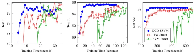
Figure 2: Comparisons between the testing performance of DCD-SSVM, FW-Struct and SVM-Struct. Note that DCD-SSVM often obtain a better model with much less training time when comparing to SVM-Struct.
4.2 Features and Inference Algorithms
For the sequence labeling tasks, NER and POS, we followed the discriminative HMM settings used in (Joachims et al., 2009) and defined the features as
Φ(x,y) =
N
X
i=l
Φemi(xi, yi)
[yi= 1][yi−1 = 1]
[yi= 1][yi−1 = 2]
. . .
[yi=k][yi−1 =k]
,
whereΦemiis the feature vector dedicated to thei-th token (or, the emission features),N represents the
number of tokens in this sequence,yi represents the
i-th token in the sequencey,[yi = 1]is the indictor
variable andkis the number of tags.
The inference problems are solved by the Viterbi algorithm. The emission features used in both POS and NER are the standard ones, including word fea-tures, word-shape feafea-tures, etc. For NER, we used additional simple gazetteer features7and word clus-ter features (Turian et al., 2010)
For dependency parsing, we followed the setting described in (McDonald et al., 2005) and used sim-ilar features. The decoding algorithm is the first-order Eisner’s algorithm (Eisner, 1997).
4.3 Algorithms and Implementation Detail
For all SSVM algorithms (including SGD),C was
chosen among the set{0.01,0.05,0.1,0.5,1,5} ac-cording to the accuracy/F1 on the development set.
For each task, the same features were used by all 7Adding Wikipedia gazetteers would likely increase the
per-formance significantly (Ratinov and Roth, 2009).
algorithms. For NER-MUC7, NER-CoNLL and POS-WSJ, we ran the online algorithms and DCD-SSVM for 25 iterations. For DP-WSJ, we only let the algorithms run for 10 iterations as the inference procedure is very expensive computationally. The algorithms in the experiments are:
DCD Our dual coordinate descent method on the L2-Loss SSVM. For DCD-SSVM,r is set to be 5.
For both DCD-Light and DCD-SSVM , we follow the suggestion in (Joachims et al., 2009): if the value of a dual variable becomes zero, its corresponding structure will be removed from the working set to improve the speed.
SVM-Struct We used the latest (v3.10) of SVM-HMM.8This version uses the cutting plane method on a 1-slack variable formulation (Joachims et al., 2009) for the L1-Loss SSVM. SVM-Struct was plemented in C and all the other algorithms are im-plemented in C#. We did not apply SVM-Struct to DP-WSJ because there is no native implementation.
Perceptron This refers to the averaged structured Perceptron method introduced by Collins (2002). To speed up the convergence rate, we shuffle the train-ing examples at each iteration.
MIRA Margin Infused Relaxed Algorithm
(MIRA) (Crammer et al., 2005) is the online
learning algorithm that explicitly uses the notion of margin to update the weight vector. We use 1-best MIRA in our experiments. To increase
8http://www.cs.cornell.edu/People/tj/
the convergence speed, we shuffle the training examples at each iteration. Following (McDonald et al., 2005), we did not tune the C parameter for the MIRA algorithm.
SGD Stochastic gradient descent (SGD) (Bottou, 2004) is a technique for optimizing general convex functions. In this paper, we use SGD as an alterna-tive baseline for optimizing the L1-Loss SSVM ob-jective function (Eq. (2) with higne loss).9 When us-ing SGD, the learnus-ing rate must be carefully tuned. Following (Bottou, 2004), the learning rate is ob-tained by
η0
(1.0 + (η0T /C))0.75
,
where C is the regularization parameter, T is the
number of updates so far and η0 is the initial step
size. The parameterη0 was selected among the set
{2−1,2−2,2−3,2−4,2−5} by running the SGD al-gorithm on a set of 1000 randomly sampled exam-ples, and then choosing the η0 with lowest primal
objective function on these examples.
FW-Struct FW-Struct represents the Frank-Wolfe algorithm for the L1-Loss SSVM (Lacoste-Julien et al., 2013).
In order to improve the training speed, we cached all the feature vectors generated by the gold la-beled data once computed. This applied to all al-gorithms except SVM-Struct, which has its own caching mechanism. We report the performance of the averaged weight vectors for Perceptron and MIRA.
4.4 Results
We present the experimental results below on com-paring different dual coordinate descent methods, as well as comparing our main algorithm, DCD-SSVM, with other structured learning approaches.
4.4.1 Comparisons of DCD Methods
We compared three DCD methods: DCD-Light, DCD-SSVM and CPD. CPD is a cutting plane method proposed by Chang et al. (2010), which uses
9To compare with SGD using its best setting, we report only
the results of SGD on the L1-Loss SSVM as we found tuning the step size for the L2-Loss SSVM is more difficult.
a dual coordinate descent algorithm to solve the in-ternal sub-problems. We specifically included CPD as it also targets at the L2-Loss SSVM.
Because different optimization strategies will reach the same objective values eventually, compar-ing them on prediction accuracy of the final models is not meaningful. Instead, here we compare how fast each algorithm converges as shown in Figure 1. Each marker on the line in this figure represents one iteration of the corresponding algorithm. Generally speaking, CPD improves the model very slowly in the early stages, but much faster after several iter-ations. In comparison, DCD-Light often behaves much better initially, and DCD-SSVM is generally the most efficient algorithm here.
The reason behind the slow performance of CPD is clear. During early rounds of the algorithm, the weight vector is far from optimal, so it spends too much time using “bad” weight vectors to find the most violated structures. On the other hand, DCD-Light updates the weight vector more fre-quently, so it behaves much better in general. DCD-SSVM spends more time on updating models during each batch, but keeps the same amount of time doing inference as DCD-Light. As a result, it finds a better trade-off between inference and learning.
4.4.2 DCD-SSVM, SVM-Struct and FW-Struct
Joachims et al. (2009) proposed a 1-slack vari-able method for the L1-Loss SSVM. They showed that solving a 1-slack variable formulation is an order-of-magnitude faster than solving the original formulation (l-slack variables formulation).
Nev-ertheless, from Figure 2, we can see the clear ad-vantage of DCD-SSVM over SVM-Struct. Al-though using 1-slack variable has improved the learning speed, SVM-Struct still converges slower than DCD-SSVM. In addition, the performance of models trained by SVM-Struct in the early stage is quite unstable, which makes early stopping an in-effective strategy in practice when training time is limited.
0 10 20 30 76
77 78 79 80
Training Time (seconds)
Test
F1
(a) Test F1 vs. Time in NER-MUC7
0 100 200 300 400
96.6 96.8 97 97.2
Training Time (seconds)
Test
Acc
(b) Test Acc vs. Time in POS-WSJ
0 2,000 4,000 6,000
88 89 90 91
Training Time (seconds)
Test
Acc
DCD-SSVM PERP MIRA SGD
[image:10.612.88.526.54.190.2](c) Test Acc vs. Time in DP-WSJ
Figure 3: Comparisons between DCD-SSVM and popular online learning algorithms. Note that the results diverge when comparing Perceptron and MIRA. In general, DCD-SSVM is the most stable algorithm.
Task/Data DCD Percep MIRA SGD
NER-MUC7 79.4 78.5 78.8 77.8
NER-CoNLL 85.6 85.3 85.1 84.2
POS-WSJ 97.1 96.9 96.9 96.9
DP-WSJ 90.8 90.3 90.2 90.9
Table 1: Performance of online learning algorithms and the DCD-SSVM algorithm on the testing sets. NER is measured by F1while others by accuracy.
4.4.3 DCD-SSVM, MIRA, Perceptron and SGD
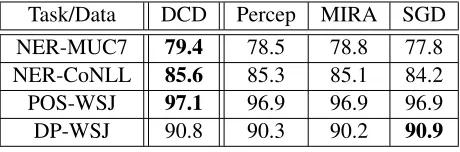
As in binary classification, large-margin methods like SVMs often perform better than algorithms like Perceptron and SGD (Hsieh et al., 2008; Shalev-Shwartz and Zhang, 2013), here we observe similar behaviors in the structured output domain. Table 1 shows the final test accuracy numbers or F1scores of
models trained by algorithms including Perceptron, MIRA and SGD, compared to those of the SSVM models trained by DCD-SSVM. Among the bench-mark datasets and tasks we have experimented with, DCD-SSVM derived the most accurate models, ex-cept for DP-WSJ when compared to SGD.
Perhaps a more interesting comparison is on the training speed, which can be observed in Fig-ure 3. Compared to other online algorithms, DCD-SSVM can take advantage of cached dual variables and structures. We show that the training speed of DCD-SSVM can be competitive to that of the on-line learning algorithms, unlike SVM-Struct. Note that SGD is not very stable for NER-MUC7, even though we tuned the step size very carefully.
5 Conclusion
In this paper, we present a novel approach for learn-ing the L2-Loss SSVM model. By combinlearn-ing the ideas of dual coordinate descent and cutting plane methods, the hybrid approach, DCD-SSVM outper-forms other SSVM training methods both in terms of objective value reduction and testing error rate reduction. As demonstrated in our experiments on several NLP tasks, our approach also tends to learn more accurate models than commonly used structured learning algorithms, including structured Perceptron, MIRA and SGD. Perhaps more inter-estingly, our SSVM learning method is very effi-cient: the model training time is competitive to on-line learning algorithms such as structured Percep-tron and MIRA. These unique qualities make DCD-SSVM an excellent choice for solving a variety of complex NLP problems.
In the future, we would like to compare our algo-rithm to other structured prediction approaches, such as conditional random fields (Lafferty et al., 2001) and exponential gradient descent methods (Collins et al., 2008). Expediting the learning process fur-ther by leveraging approximate inference is also an interesting direction to investigate.
Acknowledgments
[image:10.612.72.302.243.319.2]References
B. Bohnet. 2010. Very high accuracy and fast depen-dency parsing is not a contradiction. InProceedings of the 23rd International Conference on Computational Linguistics, Proceedings the International Conference on Computational Linguistics (COLING).
L. Bottou. 2004. Stochastic learning. In Olivier Bous-quet and Ulrike von Luxburg, editors,Advanced Lec-tures on Machine Learning, Lecture Notes in Artifi-cial Intelligence, LNAI 3176, pages 146–168. Springer Verlag, Berlin.
M. Chang, V. Srikumar, D. Goldwasser, and D. Roth. 2010. Structured output learning with indirect super-vision. InProceedings of the International Conference on Machine Learning (ICML).
T. Cohn and M. Lapata. 2009. Sentence compression as tree transduction. Journal of AI Research, 34:637– 674, April.
M. Collins, A. Globerson, T. Koo, X. Carreras, and P. L. Bartlett. 2008. Exponentiated gradient algorithms for conditional random fields and max-margin Markov networks. Journal of Machine Learning Research, 9. M. Collins. 2002. Discriminative training methods for
hidden Markov models: Theory and experiments with perceptron algorithms. InProceedings of the Confer-ence on Empirical Methods for Natural Language Pro-cessing (EMNLP).
K. Crammer, R. Mcdonald, and F. Pereira. 2005. Scal-able large-margin online learning for structured clas-sification. Technical report, Department of Computer and Information Science, University of Pennsylvania. J. Desrosiers and M. E. L¨ubbecke. 2005. A primer in
column generation. InColumn Generation, pages 1– 32. Springer.
J. M. Eisner. 1997. Three new probabilistic models for dependency parsing: An exploration. InProceedings the International Conference on Computational Lin-guistics (COLING), pages 340–345.
Y. Freund and R. Schapire. 1999. Large margin clas-sification using the Perceptron algorithm. Machine Learning, 37(3):277–296.
C.-J. Hsieh, K.-W. Chang, C.-J. Lin, S. S. Keerthi, and S. Sundararajan. 2008. A dual coordinate descent method for large-scale linear SVM. In Proceedings of the International Conference on Machine Learning (ICML), New York, NY, USA. ACM.
T. Joachims, T. Finley, and Chun-Nam Yu. 2009. Cutting-plane training of structural SVMs. Machine Learning, 77(1):27–59.
J. Kivinen and M. K. Warmuth. 1995. Exponentiated gradient versus gradient descent for linear predictors. InACM Symp. of the Theory of Computing.
T. Koo, A. Globerson, X. Carreras, and M. Collins. 2007. Structured prediction models via the matrix-tree theo-rem. InProceedings of the 2007 Joint Conference of EMNLP-CoNLL, pages 141–150.
C. Kruengkrai, K. Uchimoto, J. Kazama, Y. Wang, K. Torisawa, and H. Isahara. 2009. An error-driven word-character hybrid model for joint chinese word segmentation and pos tagging. InProceedings of the Annual Meeting of the Association for Computational Linguistics (ACL), pages 513–521.
S. Lacoste-Julien, M. Jaggi, M. W. Schmidt, and P. Pletscher. 2013. Stochastic block-coordinate Frank-Wolfe optimization for structural SVMs. In Pro-ceedings of the International Conference on Machine Learning (ICML).
J. Lafferty, A. McCallum, and F. Pereira. 2001. Con-ditional random fields: Probabilistic models for seg-menting and labeling sequence data. InProceedings of the International Conference on Machine Learning (ICML).
D. D. Lewis, Y. Yang, T. Rose, and F. Li. 2004. RCV1: A new benchmark collection for text categorization research. Journal of Machine Learning Research, 5:361–397.
L. Li, K. Zhou, G.-R. Xue, H. Zha, and Y. Yu. 2009. Enhancing diversity, coverage and balance for summa-rization through structure learning. InProceedings of the 18th international conference on World wide web, The International World Wide Web Conference, pages 71–80, New York, NY, USA. ACM.
Z.-Q. Luo and P. Tseng. 1993. Error bounds and conver-gence analysis of feasible descent methods: A general approach.Annals of Operations Research, 46(1):157– 178.
M. P. Marcus, B. Santorini, and M. Marcinkiewicz. 1993. Building a large annotated corpus of En-glish: The Penn Treebank. Computational Linguistics, 19(2):313–330, June.
A. F. Martins, K. Gimpel, N. A. Smith, E. P. Xing, M. A. Figueiredo, and P. M. Aguiar. 2010. Learning struc-tured classifiers with dual coordinate ascent. Technical report, Technical report CMU-ML-10-109.
R. McDonald, K. Crammer, and F. Pereira. 2005. Online large-margin training of dependency parsers. In Pro-ceedings of the Annual Meeting of the Association for Computational Linguistics (ACL), pages 91–98, Ann Arbor, Michigan.
R. C. Moore, W. Yih, and A. Bode. 2007. Improved dis-criminative bilingual word alignment. InProceedings of the Annual Meeting of the Association for Compu-tational Linguistics (ACL).
L. Ratinov and D. Roth. 2009. Design challenges and misconceptions in named entity recognition. InProc. of the Annual Conference on Computational Natural Language Learning (CoNLL), Jun.
N. Ratliff, J. Andrew (Drew) Bagnell, and M. Zinkevich. 2007. (Online) subgradient methods for structured prediction. InProceedings of the International Work-shop on Artificial Intelligence and Statistics, March. S. Shalev-Shwartz and Y. Singer. 2006. Online
learn-ing meets optimization in the dual. InProceedings of the Annual ACM Workshop on Computational Learn-ing Theory (COLT).
S. Shalev-Shwartz and T. Zhang. 2013. Stochastic dual coordinate ascent methods for regularized loss min-imization. Journal of Machine Learning Research, 14:567–599.
S. Shalev-Shwartz, Y. Singer, and N. Srebro. 2007. Pe-gasos: primal estimated sub-gradient solver for SVM. In Zoubin Ghahramani, editor,Proceedings of the In-ternational Conference on Machine Learning (ICML), pages 807–814. Omnipress.
S. Shevade, P. Balamurugan, S. Sundararajan, and S. Keerthi. 2011. A sequential dual method for struc-tural SVMs. In IEEE International Conference on Data Mining(ICDM).
E. F. T. K. Sang and F. De Meulder. 2003. Introduction to the CoNLL-2003 shared task: Language-independent named entity recognition. In Walter Daelemans and Miles Osborne, editors,Proceedings of CoNLL-2003, pages 142–147. Edmonton, Canada.
B. Taskar, C. Guestrin, and D. Koller. 2004a. Max-margin markov networks. In The Conference on Advances in Neural Information Processing Systems (NIPS).
B. Taskar, D. Klein, M. Collins, D. Koller, and C. Man-ning. 2004b. Max-margin parsing. In Proceedings of the Conference on Empirical Methods for Natural Language Processing (EMNLP).
B. Taskar, S. Lacoste-julien, and M. I. Jordan. 2005. Structured prediction via the extragradient method. In
The Conference on Advances in Neural Information Processing Systems (NIPS).
B. Taskar, S. Lacoste-Julien, and M. I Jordan. 2006. Structured prediction, dual extragradient and bregman projections. Journal of Machine Learning Research, 7:1627–1653.
I. Tsochantaridis, T. Hofmann, T. Joachims, and Y. Altun. 2004. Support vector machine learning for interde-pendent and structured output spaces. InProceedings
of the International Conference on Machine Learning (ICML).
J. Turian, L. Ratinov, and Y. Bengio. 2010. Word rep-resentations: a simple and general method for semi-supervised learning. In Proceedings of the Annual Meeting of the Association for Computational Linguis-tics (ACL), pages 384–394, Stroudsburg, PA, USA. Association for Computational Linguistics.
Po-Wei Wang and Chih-Jen Lin. 2013. Iteration com-plexity of feasible descent methods for convex opti-mization. Technical report, National Taiwan Univer-sity.