Learning Strictly Local Subsequential Functions

Learning Strictly Local Subsequential Functions

Jane Chandlee University of Delaware Department of Linguistics

and Cognitive Science 125 East Main Street

Newark, DE 19716 [email protected]

R´emi Eyraud QARMA team Laboratoire d’Informatique

Fondamentale Marseille, France remi.eyraud@ lif.univ-mrs.fr

Jeffrey Heinz University of Delaware Department of Linguistics

and Cognitive Science 125 East Main Street

Newark, DE 19716 [email protected]

Abstract

We define two proper subclasses of sub-sequential functions based on the concept of Strict Locality (McNaughton and Papert, 1971; Rogers and Pullum, 2011; Rogers et al., 2013) for formal languages. They are called Input and Output Strictly Local (ISL and OSL). We provide an automata-theoretic characterization of the ISL class and theorems establishing how the classes are related to each other and to Strictly Local languages. We give evidence that local phonological and morpho-logical processes belong to these classes. Fi-nally we provide a learning algorithm which provably identifies the class of ISL functions in the limit from positive data in polynomial time and data. We demonstrate this learning result on appropriately synthesized artificial corpora. We leave a similar learning result for OSL functions for future work and sug-gest future directions for addressing non-local phonological processes.

1 Introduction

In this paper we define two proper subclasses of sub-sequential functions based on the properties of the well-studied Strictly Local formal languages (Mc-Naughton and Papert, 1971; Rogers and Pullum, 2011; Rogers et al., 2013). These are languages that can be defined with grammars of substrings of length k (calledk-factors), such that a string is in the language only if its ownk-factors are a subset of the grammar. These languages have also been char-acterized by Rogers and Pullum (2011) as those that

have the property expressed in the following theo-rem (which can be taken as a defining property):

Theorem 1 (Suffix Substitution Closure). L is Strictly Local iff for all stringsu1,v1,u2,v2, there

exists k ∈ N such that for any string x of length

k−1, ifu1xv1,u2xv2 ∈L, thenu1xv2∈L.

These languages can model natural language phonotactic constraints which pick out contiguous substrings bounded by some lengthk(Heinz, 2007; Heinz, 2010). We define Input Strictly Local (ISL) and Output Strictly Local (OSL) functions which model phonological processes for which the target and triggering context are a bounded contiguous substring. Here our use of ‘process’ is not specific to rule-based grammatical formalisms (such as SPE (Chomsky and Halle, 1968)). ISL and OSL func-tions modelmappingsfrom underlying forms to sur-face forms, which are also the bedrock of constraint-based frameworks like Optimality Theory (Prince and Smolensky, 1993).

By showing that local phonological processes can be modeled with ISL (and OSL) functions, we pro-vide the strongest computational characterization of the input-output mappings these processes repre-sent. While it has been shown that phonological mappings describable with rules of the form A → B / C D (where A, B, C, and D are regular languages) are regular (Johnson, 1972; Kaplan and Kay, 1994), and even subsequential (Chandlee and Heinz, 2012; Heinz and Lai, 2013), many logically possible regular and subsequential mappings are not plausible phonological mappings. Since these im-plausible mappings cannot be modeled with ISL or OSL functions, we provide a more precise notion of

what constitues plausible phonological mappings. In addition, we present the Input SL Function Learning Algorithm (ISLFLA) and prove that it identifies this class in the limit (Gold, 1967) in poly-nomial time and data (de la Higuera, 1997). Our approach follows previous work on learning subse-quential transductions, namely Oncina et al. (1993), Oncina and Var`o (1996), Castellanos et al. (1998), and Gildea and Jurafsky (1996). Oncina et al. (1993) present OSTIA (Onward Subsequential Transducer Inference Algorithm), an algorithm that learns the class of subsequential functions in the limit from positive data. OSTIA is only guaranteed to identify total functions exactly, but Oncina and Var`o (1996) and Castellanos et al. (1998) present the modifica-tions OSTIA-N, OSTIA-D, and OSTIA-R, which learn partial functions using negative data, domain information, and range information, respectively.

In terms of linguistic applications, Gildea and Jurafsky (1996) show that OSTIA fails to learn the phonological mapping of English flapping when given natural language data. The authors modified OSTIA with three learning heuristics (context, com-munity, and faithfulness) and showed that the mod-ified learner successfully learns flapping and sev-eral other phonological rules. Context encodes the idea that phonological changes depend on the con-text of the segment undergoing the change. Commu-nitygives the learner the ability to deduce that seg-ments belonging to a natural class are likely to be-have similarly. Lastly,faithfulness, by which under-lying segments are assumed to be realized similarly on the surface, was encoded with a forced alignment between the input-output strings in the data set.1 We believe this alignment removes OSTIA’s guarantee that all subsequential functions are learned.

Similar to the approach of Gildea and Jurafsky (1996), our learner employs a context bias because it knows its target is an ISL function and therefore the transduction only involves bounded contiguous substrings. And similar to OSTIA-D (Oncina and Var`o, 1996; Castellanos et al., 1998), the ISLFLA makes use of domain information, because it makes decisions based on the input strings of the data set. It also employs a faithfulness bias in terms of the

prop-1_{The alignment was similar to the string-edit distance}

mehod used in Hulden et al. (2011).

ertyonwardness(see§2). The ISLFLA is supported by a theoretical result like Oncina et al. (1993), but learns a more restrictive class of mappings. We be-lieve the theoretical results for this class will lead to new algorithms which include something akin to the community bias and that will succeed on natural lan-guage data while keeping strong theoretical results.

The proposed learner also builds on earlier work by Chandlee and Koirala (2014) and Chandlee and Jardine (2014) which also used strict locality to learn phonological processes but with weaker theoretical results. The former did not precisely identify the class of functions the learner could learn, and the latter could only guarantee learnability of the ISL functions with a closed learning sample.

The paper is organized as follows.§2 presents the mathematical notations to be used. §3 defines ISL and OSL functions, provides an automata-theoretic characterization for ISL, and establishes some prop-erties of these classes. §4 demonstrates how these functions can model local phonological processes, including substitution, insertion, and deletion. §5 presents the ISLFLA, proves that it efficiently learns the class of ISL functions, and provides demonstra-tions.§6 concludes.

2 Preliminaries

The set of all possible finite strings of symbols from a finite alphabetΣand the set of strings of length≤ nareΣ∗ andΣ≤n_{, respectively. The unique empty}

string is represented withλ. The length of a stringw is|w|, so|λ|=0. The set of prefixes ofw,Pref(w), is{p∈Σ∗ |(∃s∈Σ∗)[w=ps]}, and the set of suf-fixes ofw,Suff(w), is_{s _∈ Σ∗ _{|(∃p ∈ Σ}∗_{)[w =}

ps]}. For allw ∈ Σ∗ andn ∈ N, Suffn(w)is the single suffix ofwof lengthnif|w| ≥n; otherwise

Suffn(w) = w. If w = ps, then ws−1 _{= p and}

p−1w = s. The longest common prefix of a set of stringsS,lcp(S), isp ∈ ∩w∈SPref(w)such that

∀p0 _{∈ ∩}

w∈SPref(w),|p0|<|p|.

A functionf with domain A and co-domain B is writtenf : A _→ B. We sometimes writex _7→f y

forf(x) =y. When A and B are free monoids (like Σ∗), the input and output languages of a functionf are the stringsetsdom(f) ={x|(∃y)[x7→f y]}and

image(f) ={y|(∃x)[x7→f y]}, respectively.

subsequen-tial finite state transducer (SFST) is a 6-tuple (Q, q0,Σ,Γ, δ, σ), where Qis a finite set of states,

Σand Γ are finite alphabets, q0 ∈ Q is the initial

state,δ _⊆ Q_×Σ_×Γ∗_{×Qis a set of edges, and}

σ : Q → Γ∗ is the final output function that maps states to strings that are appended to the output if the input ends in that state.δrecursively defines a map-pingδ∗: (q, λ, λ, q) ∈ δ∗; if(q, u, v, q0) ∈ δ∗ and (q0, σ, w, q00) _∈ δthen(q, uσ, vw, q00) _∈δ∗. SFSTs are deterministic, which means their edges have the following property: [(q, a, u, r),(q, a, v, s) ∈ δ ⇒ u = v _∧ r = s]. Hence, we also refer to δ as the transitionfunction, and∀(q, a, u, r) _∈ δ, we let δ1(q, a) =uandδ2(q, a) =r.

The relation that a SFST _T recog-nizes/accepts/generates is

R(T) =n(x, yz)∈Σ∗×Γ∗|(∃q∈Q)

(q0, x, y, q)∈δ∗∧z=σ(q)

o .

Since SFSTs are deterministic, the relations they recognize are functions.Subsequential functionsare defined as those describable with SFSTs.

For any functionf : Σ∗ →Γ∗andx∈Σ∗, let the tailsofxwith respect tof be defined as

tailsf(x) =

(y, v)_|f(xy) =uv_∧ u=lcp(f(xΣ∗)) .

If stringsx1, x2 ∈Σ∗have the same set of tails with

respect to a functionf, they aretail-equivalentwith respect tof and we writex1 ∼f x2. Clearly,∼f is

an equivalence relation which partitionsΣ∗.

Theorem 2(Oncina and Garcia, 1991). A function f issubsequentialiff _∼f partitionsΣ∗ into finitely

many blocks.

The above theorem can be seen as the functional analogue to the MyHill-Nerode theorem for regular languages. Recall that for any stringsetL, the tails of a wordw w.r.t. L is defined as tailsL(w) =

{u _| wu _∈ L_}. These tails can be used to par-tition Σ∗ _{into a finite set of equivalence classes}

iff L is regular. Furthermore, these equivalence classes are the basis for constructing the (unique up to isomorphism) smallest deterministic acceptor for a regular language. Likewise, Oncina and Gar-cia’s proof of Theorem 2 shows how to construct the (unique up to isomorphism) smallest SFST for

a subsequential function f. We refer to this trans-ducer as the canonical transtrans-ducer forfand denote it with_TfC. The states of_TfC are in one-to-one corre-spondence withtailsf(x)for allx ∈ Σ∗ (Oncina

and Garc´ıa, 1991). To construct TC

f first let, for

all x _∈ Σ∗ anda _∈ Σ, the contribution ofaw.r.t. xbecontf(a, x) =lcp(f(xΣ∗)−1lcp(f(xaΣ∗)).

Then,

• Q=_{tailsf(x)|x∈Σ∗},

• q0 =tailsf(λ),

• ∀tailsf(x) ∈ Q, σ(tailsf(x)) =

lcp(f(xΣ∗))−1f(x)ifx_∈ dom(f)and is un-defined otherwise,

• δ =

(tailsf(x), a,contf(a, x),

tailsf(xa))}.

TC

f has an important property calledonwardness.

Definition 1 (onwardness). For all q _∈ Q let the outputs of the edges out of q be outs(q) =

u | (∃a ∈Σ)(∃r ∈ Q)[(q, a, u, r) ∈ δ] . A SFST_T is onwardif for allq_∈Q_{\ {}q0},lcp(outs(q)) =λ.

Informally, this means that the writing of output is never delayed. Readers are referred to Oncina and Garc´ıa (1991), Oncina et al. (1993), and Mohri (1997) for more on SFSTs.

3 Strictly Local Functions

In this section we define Input and Output Strictly Local functions and provide properties of these classes. These definitions are analogous to the language-theoretic definition of Strictly Local lan-guages (Theorem 1) (Rogers and Pullum, 2011; Rogers et al., 2013).

Definition 2(Input Strictly Local Function). A func-tion f is Input Strictly Local (ISL) if there is a k such that for all u1, u2 ∈ Σ∗, if Suffk−1(u1) = Suffk−1(u2)thentailsf(u1) =tailsf(u2).

The theorem below establishes an automata-theoretic characterization of ISL functions.

Theorem 3. A functionf is ISL iff there is somek such thatf can be described with a SFST for which

1. Q= Σ≤k−1_andq 0 =λ

2. (_∀q_∈Q,_∀a_∈Σ,_∀u_∈Γ∗₎

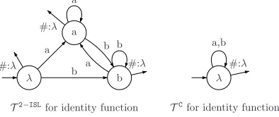
This theorem helps make clear how ISL functions are Markovian: the output for input symbol a de-pends on the last(k₋1)input symbols. Also, since the transducer defined in Theorem 3 is determinis-tic, it is unique and we refer to it asTISL

f .TfISLmay

not be isomorphic toTC

f . Figure 1 showsTfISL(with

k= 2) andTC

f for the identity function.2

a

b λ

a b a

b #:λ

#:λ #:λ

a

b

T2−ISL_{for identity function}

λ #:λ a,b

TC_{for identity function}

1

Figure 1: Non-isomorphic_TISL

f (left) andTfC(right)

Before we present the proof of Theorem 3, we make the following remarks, and then prove a lemma.

Remark 1. For alln, m _∈Nwithn≤ m, and for

allw_∈ Σ∗_,

Suffn(Suffm(w)) =Suffn(w)since bothwandSuffm(w)share the samen-long suffix.

Remark 2. For all w, v _∈ Σ∗, k _∈ N,

Suffk−1 Suffk−1(w)v = Suffk−1(wv). This is a direct consequence of Remark 1.

Lemma 1. Let_T be a SFST constructed as in The-orem 3. If(λ, w, u, q)inδ∗_{thenq =Suff}k−1_(w).

Proof. The proof is by induction on δ∗. The base case follows from the facts that(λ, λ, λ, λ)_∈δ∗(by definition ofδ∗_{), and thatλ=}

Suffk−1(λ).

Next assume the inductive hypothesis (IH) that there existsw_∈Σ∗_,u∈Γ∗_{, such that(λ, w, u, q)∈}

δ∗ implies q = Suffk−1(w). We show ∀a ∈ Σ, ∀x _∈ Γ∗ that (λ, wa, ux, q0) _∈ δ∗ implies q0 =

Suffk−1(wa). Now (λ, w, u,Suffk−1(w)) ∈ δ∗

(by IH) so(Suffk−1(w), a, x, q0)∈δ. By construc-tion of_T,q0 =Suffk−1(Suffk−1(w)a), which by Remark 2, equalsSuffk−1(wa).

Proof of Theorem 3. (⇐) Fixk _∈ Nand let f be a

function described byT = {Q, q0,Σ,Γ, δ, σ}

con-structed as in Theorem 3. Let w1, w2 ∈ Σ∗ such

thatSuffk−1(w1) = Suffk−1(w2). By Lemma 1, 2

In all figures, single-symbol transition labels indicate that the input and output are identical, and the final output function is represented as a transition on the end-of-word symbol #.

bothw1andw2 lead to the same state and therefore tailsf(w1) =tailsf(w2). Thusf isk-ISL.

(_⇒) Consider any ISL function f. Then there is a k such that (_∀w1, w2 ∈ Σ∗)[Suffk−1(w1) = Suffk−1(w2) ⇒tailsf(w1) = tailsf(w2)]. We

show that_TfISL exists. Since Σ≤k−1 _{is a finite set,}

the equivalence relation ∼f partitions Σ∗ into at

most |Σ≤k−1_{| blocks. Hence by Theorem 2, f is}

subsequential and a canonical subsequential trans-ducerTC

f ={Qc, q0c,Σ,Γ, δc, σc}exists.

ConstructT ={Q, q0,Σ,Γ, δ, σ}as follows:

• Q= Σ≤k−1_andq 0 =λ

• ∀q ∈ Q, σ(q) = σc tailsf(q)

iff(q)is de-fined, elseσ(q)is undefined.

• ∀q _∈ Q, _∀a _∈ Σ, ∀u _∈ Γ∗_,

q, a, u,Suffk−1(qa)

∈ δ iff

tailsf(q), a, u,tailsf(qa)

∈δc.

First, by its construction, the states and transitions of_T meet requirements (1) and (2) of Theorem 3.

Next, we show that T computes the same function as TC

f. We first establish by

induc-tion on δ∗ the following (?): _∀w _∈ Σ∗, ∀u _∈ Γ∗_{, q}

0, w, u,Suffk−1(w)

∈ δ∗ _iff tailsf(λ), w, u,tailsf(w)

∈δ_c∗. Clearly tailsf(λ), λ, λ,tailsf(λ)

∈ δ∗_c and λ, λ, λ, λ

∈δ∗ _{by definition of the extended}

tran-sition function. Thus the base case is satisfied. Next assume the inductive hypothesis (IH) for w _∈ Σ∗ _{and u ∈ Γ}∗_{. We show ∀a ∈ Σ and}

∀x ∈ Γ∗ that λ, wa, ux,Suffk−1(wa)

∈ δ∗ iff

tailsf(λ), wa, ux,tailsf(wa)

∈δ∗_c. Suppose tailsf(λ), wa, ux,tailsf(wa)

∈ δ_c∗. By IH, tailsf(λ), w, u,tailsf(w)

∈ δ_c∗; hence tailsf(w), a, x,tailsf(wa)

∈δc.

Let q = Suffk−1(w). Observe that

Suffk−1(w) = Suffk−1(q) by Remark 1. Conse-quently, sincef isk-ISL,tailsf(w) =tailsf(q).

Similarly, Suffk−1(wa) = Suffk−1(qa) and thus

tailsf(wa) = tailsf(qa). By substitution then,

we have tailsf(λ), w, u,tailsf(q)

∈ δ_c∗ and

tailsf(q), a, x,tailsf(qa)

∈δc.

By construction of T, q, a, x,Suffk−1(qa) ∈ δ. By IH, λ, w, u,Suffk−1(w)

= λ, w, u, q ∈ δ∗_{. Thus, λ, wa, ux,}

Suffk−1(qa) ∈ δ∗ which is the same as saying λ, wa, ux,Suffk−1(wa)

∈δ∗. Conversely, consider any a _∈ Σ and x _∈ Γ∗ _{and suppose λ, wa, ux,}

By IH, λ, w, u,Suffk−1(w) ∈ δ∗; hence

Suffk−1(w), a, x,Suffk−1(wa)

∈ δ. As be-fore, letting q = Suffk−1(w), it follows that

Suffk−1(w) = Suffk−1(q) so tailsf(w) =

tailsf(q), and Suffk−1(wa) = Suffk−1(qa)

so tailsf(wa) = tailsf(qa). Therefore,

q, a, x,Suffk−1(qa)∈δ.

By construction of T, this means

tailsf(w), a, x,tailsf(wa)

∈ δc. By IH,

tailsf(λ), w, u,tailsf(w)

∈ δ∗

c. By the

defi-nition of the extended transition function, it follows that tailsf(λ), wa, ux,tailsf(wa)

∈δ∗_c. This completes the induction, establishing (?).

Letw ∈Σ∗. Iff(w)is defined thenf(w) =uv where tailsf(λ), w, u,tailsf(w)

∈ δ_c∗ and σc tailsf(w)

= v. From (?), we know λ, w, u,Suffk−1(w)

∈ δ∗. Also, σ Suffk−1(w)

= σc tailsf(Suffk−1(w))

. Since f is k-ISL, tailsf(w) =

tailsf(Suffk−1(w)) (cf. Remark 1). Thus

σ Suffk−1(w)

= σc tailsf(w)

= v. There-foreT(w) =uvalso.

If f(w) is not defined then there are two cases. Case 1: tailsf(λ), w, u,tailsf(w)

6∈ δ∗

c. By the above lemma, it follows

λ, w, u,Suffk−1(w)

6∈δ∗and soT(w)is also de-fined. Case 2: tailsf(λ), w, u,tailsf(w)

∈δ_c∗ but σc(tailsf(w)) is undefined. By construction

ofT,σ(Suffk−1(w))is also undefined.

Similar to Definition 2 above, the following defi-nition of OSL functions says that if the outputs of two input strings share the same suffix of length (k₋1), then those inputs have the same tails.

Definition 3 (Output Strictly Local Function). A functionfis Output Strictly Local (OSL) if there is a ksuch that for allu1, u2 ∈Σ∗, ifSuffk−1(f(u1))= Suffk−1(f(u2))thentailsf(u1) =tailsf(u2).

The automata-theoretic characterization of this class is left as future work.

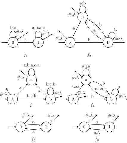
Next, some properties of ISL and OSL functions are identified. The proofs of the following theorems will refer to the example SFSTs in Figure 2.

First we establish that ISL and OSL functions are proper subclasses of the subsequential functions. (They are subclasses by definition.)

Theorem 4. There are subsequential functions which are neither ISL nor OSL.

0 a 1

#:λ #:λ b,c a,b:a,c f1 a b λ b a a b #:λ #:λ #:λ a:b b f2 1 a b λ a a b,c:b #:λ #:λ #:λ a,b:a,c:a b,c:b f3 a b λ b a:aa a:aa b #:λ #:λ #:λ a:aa b f4 1 0 1 a #:λ #:a

a f5 1 0 a a:λ #:λ #:λ f6 1

Figure 2: Examples for proofs of Theorems 4-7

Proof. Consider the subsequential function f1 in

Figure 2 and choose any k _∈ N. Since

f1(bckb) = bckb andf1(ackb) = ackait follows

thattailsf1(bc

k_)6=tails f1(ac

k_{)even though}

in-puts bck _andack _{share a common suffix of length}

(k − 1). Likewise, the outputs of these inputs f1(bck) =bckandf1(ack) = ack share a common

suffix of length (k₋1), but the tails of these inputs, as mentioned, are distinct. Hence by Definitions 2 and 3, there is nokfor whichf1is ISL or OSL. Theorem 5. The class of ISL functions is incompa-rable to the class of OSL functions.

Proof. Considerf2in Figure 2. This function is ISL

by Theorem 3. However it is not OSL. Consider any k_∈N. Observe thatf2(aak) =f2(abk) =abkand

so the outputs share the same suffix of length (k− 1). However,tailsf2(aa

k_{) 6= tails} f2(ab

k_{) since}

(a, b)_∈tailsf2(aa

k_{)but(a, a)∈}

tailsf2(ab

k_).

Similarly, considerf3in Figure 2. This function is

2-OSL because inputs mapped to outputs which end inahave the same tails (i.e., they all lead to statea), and inputs mapped to outputs ending inbhave the same tails.

However, f3 is not ISL. Consider any k ∈ N. The inputs cbk and abk share the same

suf-fix of length (k ₋1). However, tailsf3(cb

tailsf3(ab

k_{) since (b, b) ∈}

tailsf3(cb

k_{) but}

(b, a)∈tailsf3(ab

k_).

Finally, the two classes are obviously not disjoint, since the identity function is both ISL and OSL.

Theorem 6. The output language of an ISL or OSL function is not necessarily a Strictly Local language.

Proof. Consider f4 in Figure 2. By Theorem 3, it

is ISL. It is also 2-OSL since inputs mapped to out-puts which end inahave the same tails (i.e., they all lead to statea). Similarly, inputs mapped to outputs ending inbhave the same tails.

Letk _∈ N. Observe thatf4(ak) = a2k and

fur-ther that fur-there is no inputxandksuch thatf4(x) =

a2k+1_{. Sincea}2k _{= a}k−1_ak_{a = a}k−2_ak_{aa, if the}

output language off4 were SL it would follow, by

Theorem 1, that ak−1_ak_{aa = a}2k+1 _{also belongs}

to the output language. But there is no input inΣ∗ whichf4maps to an odd sequence ofa’s.

Theorem 7. If either the output or input language of a subsequential functionf is Strictly Local then it does not follow thatfbelongs to either ISL or OSL.

Proof. LetΣ = Γ =_{a_}and consider the function f5 which, for alln∈ N, mapsantoanifnis even

andan _{to a}n_{aif n is odd. f}

5 is subsequential, as

shown in Figure 2, and its domain,a∗_{, is a Strictly}

Local language. However,f5is neither ISL nor OSL

for anyksince thetailsofa2k_{includes(λ, λ)but}

thetailsofaa2k_{includes(λ, a).}

Next considerf6, which for alln∈Nmapsanto

am _{wherem= (ndiv2) ifnis even andm= (ndiv}

2)+1 ifn is odd. f6 is subsequential, as shown in

Figure 2, and theimage(f) = a∗ is Strictly Local. However,f is neither ISL nor OSL for anyksince the tailsof a2k _{includes (a, a) but the}

tails of aa2k_{includes(a, λ).}

4 Relevance to Phonology

This section will briefly discuss the range of phono-logical processes that can be modeled with ISL and/or OSL functions by providing illustrative ex-amples for three common, representative processes. These are shown in (1) with SPE-style rules.

(1) a. Devoicing: D→T / #

b. Epenthesis:∅→@/{l, r} [-coronal]

c. Deletion: {T,D} →∅/ {T, s}

See Chandlee (2014) for more details.

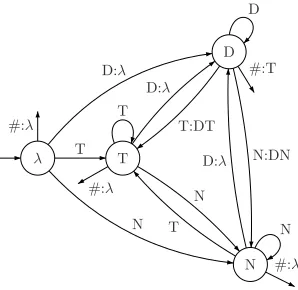
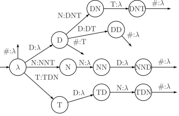
First, consider the process of final obstruent de-voicing (1-a), attested in German and other lan-guages. This process causes an underlying voiced obstruent in word-final position to surface as its voiceless counterpart. In (1-a), D abbreviates the set of voiced obstruents and T the voiceless obstruents.3 The mapping from underlying form to surface form that this process describes is represented with the 2-ISL function in Figure 3 (note N represents any sonorant).

λ

D

N T

D:λ

N D:λ

N T T

T:DT

N:DN D:λ #:λ

#:T

#:λ #:λ

T

D

N

1 Figure 3: _TISL

f for (1-a) withk= 2andΣ ={T, D, N}

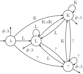
In addition to substitution processes like (1-a), an-other common type of process is insertion of a seg-ment, such as the @-epenthesis process attested in Dutch (Warner et al., 2001). This process inserts a schwa between a liquid and a non-coronal con-sonant, as specified by (1-b). Using L to represent the liquids{l, r}and K to represent any non-coronal consonant, Figure 4 presents_TfISL for this process. Following Beesley and Karttunen (2003), the sym-bol ‘?’ represents any segment of the alphabet other than the ones for which transitions are defined.4

Lastly, an example deletion process from Greek (Joseph and Philippaki-Warburton, 1987) deletes in-terdental fricatives before /T/ or /s/, as in (1-c). Fig-ure 5 presentsTISL

f for this process.

3

These abbreviations serve to improve the readability of the FST - it is assumed that the transduction replaces a given voiced obstruent with its voiceless counterpart (not with any voiceless obstruent).

4

This means Figure 4 is actually a shorthand forTISL

f , which

λ

K

? L

K:@K

? K

? L L

L

? K #:λ

#:λ

#:λ #:λ

L

K

?

1

Figure 4:_TfISLfor (1-b) withk= 2andΣ =_{L, K, ?_}

λ

D

s

?

T D:λ

s

?

T:λ

s

?:T? s

D:λ

?:D?

D:λ

T:λ

T:λ

D:T T:λ s _?

#:D

#:λ

#:λ

#:λ T #:T

:λ

s

?

D

1

Figure 5:_TfISLfor (1-c) withk= 2andΣ ={T,D, s, ?_}

The German, Dutch, and Greek examples demon-strate how ISL functions can be used to model the input-output mapping of a phonological rule. Be-yond substitution, insertion, and deletion, it is shown in Chandlee (2014) that ISL and/or OSL functions can also model many metathesis patterns, specifi-cally those for which there is an upper bound on the amount of material that intervenes between a segment’s original and surface positions (this ap-pears to include all synchronic patterns). In addi-tion, morpho-phonological processes such as local partial reduplication (i.e., in which the reduplicant is affixed adjacent to the portion of the base it was copied from) and general affixation are also shown to be ISL or OSL. More generally, we currently con-jecture that a SPE-style rewrite rule of the form A → B/ C D which applies simultaneously (left-to-right) describes an Input (Output) Strictly Local function iff there is aksuch that for allw∈ CAD it is the case that_|w_{| ≤} k. We refer readers to Ka-plan and Kay (1994) and Hulden (2009) for more

on how SPE rules and application modes determine mappings.

In contrast, non-local (long-distance) processes such as vowel harmony with transparent vowels (Gainor et al., 2012; Heinz and Lai, 2013), long dis-tance consonant harmony (Hansson, 2001; Rose and Walker, 2004; Luo, 2013) and dissimilation (Suzuki, 1998; Bennett, 2013; Payne, 2013), unbounded dis-placement/metathesis (Chandlee et al., 2012; Chan-dlee and Heinz, 2012), non-local partial reduplica-tion (Riggle, 2003), and some tonal patterns (Jar-dine, 2013) cannot be modeled with ISL or OSL functions. In §6 we comment on the potential for adapting the current analysis to non-local mappings. The next section presents a learning algorithm for ISL functions, the ISLFLA. The development of a corresponding algorithm for OSL functions is the subject of ongoing work, but see_§6 for comments.

5 Learning Input Strictly Local Functions

We now present a learning algorithm for the class of ISL functions that uses its defining property as an in-ductive principle to generalize from a finite amount of data to a possibly infinite function. This learner begins with a prefix tree representation of this data and then generalizes by merging states.5 Its state merging criterion is based on the defining property of ISL functions: two input strings with the same suffix of length(k₋1)have the same tails. The next section explains in detail how the algorithm works.

5.1 The Algorithm: ISLFLA

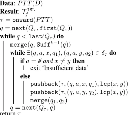
Given a finite datasetDof input-output string pairs (w, w0)such that f(w) = w0, wheref is the target function, the learner tries to build_TfISL. The dataset is submitted to the learner in the form of a prefix tree transducer (PTT), which is defined in Definition 4.

Definition 4(Prefix Tree Transducer). Aprefix tree transducerfor finite setD=_{(w, w0_{)|f(w) =w}0_}

for somef isP T T(D) = (Q, q0,Σ,Γ, δ, σ), where

• Q=S

{Pref(w)|(w, w0)∈D}andq0=λ

• δ={(u, a, λ, ua)|u, ua∈Q} • σ(w) =w0 for all(w, w0)∈D

5_{This general strategy is common in grammatical inference.}

As an example, the sample of data in (2) exempli-fies the final devoicing rule in (1-a). Figure 6 gives the PTT for this data.

(2) {(D, T), (DD, DT), (DNT, DNT), (NND, NNT), (TDN, TDN)_}

λ

D

N

T TD TDN

NN NND

DD

DN T:λ DNT#:DNT

D:λ N:λ

#:DT #:T

N:λ D:λ #:NNT

#:TDN N:λ

D:λ D:λ

N:λ T:λ #:λ

1

Figure 6: PTT for the data in (2)

Given such a PTT, the learner’s first step is to make it onward. In the PTT, the output string is with-held until the end of the input (i.e., #) is reached. In the onward version (shown in Figure 7), output is advanced as close to the root as possible. This in-volves determining thelcpof all the output strings of all outgoing transitions of a state (starting from the leaves) and suffixing that lcp to the output of the single incoming transition of the state.

λ

D

N

T

TD TDN

NN NND

DD

DN T:λ DNT #:λ

D:DT N:DNT

#:λ #:T

N:λ D:λ #:λ

#:λ N:λ

D:λ D:λ

N:NNT

T:TDN #:λ

Figure 7: Onward version of the PTT in Figure 6

Once the learner has constructed this onward rep-resentation of the data, it begins to merge states, using two nested loops. The outer loop proceeds through the entire state set (ordered lexicographi-cally) and merges each state with the state that cor-responds to its (k₋1)-length suffix. For example, for final devoicing k = 2, so each state will be merged with the state that represents its final sym-bol. This merging may introduce non-determinism, which must be removed since by definitionTISL

f is

deterministic. Non-determinism is removed in the inner loop with additional state merges.

Consider the situation depicted on the lefthand side of Figure 8, which resulted from a previous merge. The non-determinism could be resolved by

0

1

2

3

4

5 D:λ

N:N D:λ

T:DT

T:DTN 0

1

2

3

4

5 D:N N:NN

D:λ

T:DT

T:DT

1

Figure 8: Before (left) and after (right)pushback

merging states 1 and 2, except for the fact that the output strings of the two transitions differ. Before merging 1 and 2, therefore, the learner performs an operation called pushback that retains the lcp of the two output strings and prefixes what’s left to all output strings of all outgoing transitions from the re-spective destination states.

Definition 5 (pushback (Oncina et al., 1993)).

For SFST _T = (Q, q0,Σ,Γ, δ, σ), v ∈ Σ∗, and

e = (q, a, w, q0) ∈ δ, pushback T, v, e

= (Q, q0,Σ,Γ, δ0, σ) where δ0 = (δ ∪

{q, a, wv−1, q0)} ∪ {(q0, b, vz, q00)|(q0, b, z, q00) ∈ δ})\({(q0, b, z, q00)} ∪ {e}).

In the example in Figure 8,pushbackis applied to the edges(0, T, DT,1)and(0, T, DT N,2). Only thelcpof the output strings, which is DT, is retained as the output string of both edges. The remainder (which is λ and N, respectively) is prefixed to the output string of all transitions leaving the respective destination state. The result is shown on the right-hand side of Figure 8. Essentially, pushback ‘un-does’ onwardness when needed.

After pushback, states 1 and 2 can be merged. This removes the initial non-determinism but creates new non-determinism. The inner loop iterates un-til all non-determinism is resolved, after which the outer loop continues with the next state in the order. If the inner loop encounters non-determinism that cannot be removed, the ISLFLA exits with a mes-sage indicating that the data sample is insufficient.

Non-removable non-determinism occurs if and only if the situation depicted on the left in Figure 9 obtains. The normal procedure for removing

q #:λ

#:z q

s

t a:u

a:v

1

Figure 9: Irreparable determinism (left) and non-determinism from an outer loop merge (right).

determinism cannot be applied in this case. Assum-ingz 6= λ, all ofzwould have to be pushed back, but since this transition has no destination state there is nowhere for z to go. OSTIA handles this situ-ation by rejecting the outer loop merge that led to it, restoring the FST to its state before that merge and moving on to the next possible merge. But the ISLFLA cannot reject merges. If it could, the pos-sibility would arise that two states with the same (k −1)-length suffix would remain distinct in the final FST the learner outputs. Such a FST would not (by definition) be ISL. Therefore, the algorithm is at an impasse: rejecting a merge can lead to a ISL FST, while allowing it can lead to a non-subsequential (hence non-ISL) FST. It therefore ter-minates. Below is pseudo-code for the ISLFLA.

Data:P T T(D)

Result:TISL

f

τ =onward(P T T) q =next(Qτ,first(Qτ))

whileq <last(Qτ)do

merge(q,Suffk−1(q))

while_∃(q, a, x, q1),(q, a, y, q2)∈δτ do

ifa=# andx6=ythen

exit ‘Insufficient data’

else

pushback(τ,(q, a, x, q1),lcp(x, y)) pushback(τ,(q, a, y, q2),lcp(x, y)) merge(q1, q2)

q =next(Qτ, q)

returnτ

Algorithm 1:Pseudo-code for the ISLFLA

5.2 Learning Results

Here, we present a proof that the ISLFLA identifies the class of ISL functions in the limit from positive data, in the sense of Gold (1967), with polynomial

bounds on time and data (de la Higuera, 1997). First, we establish the notion of characteristic sample.

Definition 6(Characteristic sample). A sampleCS is characteristic of a functionffor an algorithmAif for all samplesSs.t.CS_⊆S,Areturns a represen-tationτ such that for allx∈dom(f),τ(x) =f(x), and for allx /_∈dom(f),τ(x)is not defined.

We can now define the learning criteria.

Definition 7(Identification in polynomial time and data (de la Higuera, 1997)). A class_Fof functions is identifiable in polynomial time and data using a classTof representations iff there exist an algorithm Aand two polynomialsp()andq()such that:

1. Given a sampleS of sizem for f ∈ F, A

re-turns a hypothesis in_O(p(m))time;

2. For each representationτ of sizekof a function f ∈F, there exists a characteristic sampleCS

off forAof size at most_O(q(k)).

Essentially the proof for convergence follows from the fact that given a sufficient sample the al-gorithm merges all and only states with the same (k−1)-length suffix.

Clearly, merges in the outer loop only involve states with the same (k−1)-length suffix. This is also the case for inner loop merges. Consider the scenario depicted on the right in Figure 9, in which qis a state created by an outer loop merge.

Afterpushback, statessandtwill be merged. If x=Suffk−1(q), then bothsandtmust havexaas a suffix. Since_|xa_|=k, it follows thatSuffk−1(s) =

Suffk−1(t). It also follows that additional states merged to remove non-determinism resulting from the merge of s and t will have the same suffix of length(k₋1). To show that all states with the same (k −1)-length suffix will be merged, it is shown that the ISLFLA willnever encounter the situation in Figure 9, provided the data set includes aseed de-fined as follows.

Definition 8(ISLFLA seed). Given ak-ISL function f and_TfISL, let Q0 ={q ∈ Q|δ1(q,#) 6= λ}. A

seedforf isS =S0_∪S00_{, where}

• S0=_{(w, w0)_|[w_∈Σ≤k_{∧f(w) =w}0_]

} • S00 = _{(wa, w00) _| a _∈ Σ, [w _∈ Σk _∧

Lemma 2 (Convergence). A seed for an ISL func-tionf is a characteristic sample for ISLFLA.

Proof. We show that for any ISL functionf and a dataset D that contains a seed S the output of the ISLFLA is_TfISL.

Let P T T(D) = (QP T T, q0P T T,Σ,Γ, δP T T,

σP T T) be the input to the ISLFLA and T =

(QT, q0T,Σ,Γ, δT, σT)be its output. First we show

that QT = Σ≤k−1. By Definitions 4 and 8,

Σ≤k−1 _{⊆ Q}

P T T. Since the ISLFLA only merges

states with the same (k₋1)-length suffix,Σ≤k−1

⊆ QT. Since it does not exit until all statesqhave been

merged withSuffk−1(q),QT = Σ≤k−1.

Next we show that given S, the algorithm will never need to merge two statesq1 andq2 such that

δ1(q1,#) 6= δ1(q2,#). Let δ1(q1,#) = z, and

δ1(q2,#) = xwithz 6= xandq1 = Suffk−1(q2).

By Definition 2, tailsf(q1) = tailsf(q2), so if

z6=xit must be the case thatq2does not have

tran-sitions for alla_∈ Σ. This is because the only way for the output strings of the outgoing transitions of q2 to differ from those of q1 is if fewer transitions

were present onq2when the PTT was made onward.

(By definition ofSwe knowq1has transitions for all

a ∈ Σ.) But sincetailsf(q1) = tailsf(q2), we

also know thatz=uxfor someu_∈Γ∗.

By Definition 8, all states up to lengthkhave tran-sitions for alla ∈ Σ; therefore,|q2| ≥ k+ 1. This

means_∃q0 _∈ Σk _betweenq

1 andq2, which will be

merged with some other state before q2 will. This

merge will cause non-determinism, which in turn will triggerpushbackand causeuto move further down the branch towardq2. By extension there will

be|q2| −kstates betweenq1andq2, each of which

will be merged, triggering pushbackof u, so that by the timeq1andq2are merged,δ1(q2,#) =ux=

z = δ1(q2,#). Thus, all non-determinism can be

removed, and so_T is subsequential.

It remains to show that ∀q _∈ QT, a ∈ Σ,

δ2(q, a) = Suffk−1(qa). Since state merging

pre-serves transitions, this follows from the construction ofP T T(D). By Theorem 3,T =_TISL

f .

Next we establish complexity bounds on the run-time of the ISLFLA and the size of the characteristic sample for ISL functions. We observe that both of these bounds improve the bounds of OSTIA. While not surprising, since ISL functions are less general

than subsequential functions, the result is important since it is an example of greatera prioriknowledge enabling learning with less time and data.

Letmbe the length of the longest output string in the sample and letndenote the number of states of the PTT;nis at most the sum of the lengths of the input strings of the pairs in the sample.

Lemma 3 (Polynomial time). The time complexity of the ISLFLA is in_O(n_·m_·k_{· |}Σ_|).

Proof. First, making the PTT onward can be done in O(m_·n): it consists of a depth-first parsing of the PTT from its root, with a computation at each state of the lcp of the outgoing transition outputs after the recursive computation of the function (see de la Higuera (2010), Chap. 18, for details). As the com-putation of thelcptakes at mostmsteps, and as it has to be done for each state, the complexity of this step is effectively inO(m_·n).

For the two loops, we need to find a bound on the number of merges that can occur. Statesqsuch that |q_| < k do not yield any merges in the outer loop. All other statesq0 are merged withSuffk−1(q), in the outer loop or in the inner one. The number of merges is thus bounded byn. Computing the suffix of length (k−1) of any word can be done inO(k) with a correct implementation of strings of charac-ters. The test of the inner loop can be done in con-stant time and so can themergeandpushback pro-cedures. After each merge, the test of the inner loop needs to be done at most|Σ_|times. As computing thelcp has a complexity inO(m), the overall com-plexity of the two loops is in_O(n_·m_·k_{· |}Σ_|).

The overall complexity of the algorithm is thus O(m·n+n·m·k· |Σ|) =O(n·m·k· |Σ|).

Let TISL

f = (Q, q0,Σ,Γ, δ, σ) be a target

trans-ducer. We definem = max{|u| |(q, a, u, q0) ∈ δ}, n=_|Q_|, andp=max_{|v_{| |}(q,#, v)_∈σ_}.

Lemma 4(Polynomial data). The size of the charac-teristic sample is in_O(n·|Σ|·k·m+n2_{·m+n·|Σ|·p).}

Proof. The first item of the seed,S0_{, covers all and}

only the states of the target: the left projection of these pairs is thus linear innand every right projec-tion is at mostn_·m+p. Thus the size ofS0 _{is at}

mostn·(n+n·m+p) =O(n2_·m+n·p).

Concerning the second part,S00_{, its cardinality is}

Each element of the left projection ofS00_{is of length}

(k+ 1) and each element of its right projection is at most of length(k+ 1)_·m+p. The size ofS00is thus inO(n_{· |}Σ_{| ·}(k_·m+p)).

Therefore, the size of the characteristic sample is in_O(n_·|Σ_|·k_·m+n2_{·m+n·|Σ|·p), which is clearly}

polynomial in the size of the target transducer.

Theorem 8. The ISLFLA identifies the class of ISL functions in polynomial time and data.

Proof. Immediate from Lemmas 2, 3, and 4.

5.3 Demonstrations

We tested the ISLFLA with the three examples in §4, as well as the English flapping process (t →R /

´

V V). For each case, a data set was constructed according to Definition 8 using the alphabets pre-sented in§4. The alphabet for English flapping was {_{V, V, t, ?}´ _{}. The value ofkis 2 for final devoicing,} @-epenthesis, and fricative deletion and 3 for English flapping. A few additional data points of length 5 or 6 were also added to make the data set a superset of the seed. In all four cases, the learner returned the correctTISL

f .

The decision to use artificial corpora in these demonstrations was motivated by the fact that the sample in Definition 8 will not be present in a natural language corpus. That sample includes all possible sequences of symbols from the alphabet of a given length, whereas a natural language corpus will re-flect the language-particular restrictions against cer-tain segment sequences (i.e., phonotactics).

As discussed in the introduction, Gildea and Ju-rafsky (1996) address this issue with natural lan-guage data by equipping OSTIA with a community bias, whereby segments belonging to a natural class (i.e., stops, fricatives, sonorants) are expected to be-have similarly, and a faithfulness bias, whereby seg-ments are assumed to be realized similarly on the surface. In our demonstrations we put aside the is-sue of the behavior of segments in a natural class by using abbreviated alphabets (e.g., T for all voiceless stops). But if in fact knowledge of natural classes precedes the learning of phonological processes, the use of such an alphabet is appropriate.

In future developments of the ISLFLA we like-wise aim to accommodate natural language data, but in a way that maintains the theoretical result of

identification in the limit. The restrictions on seg-ment sequences represented in natural language data amount to ‘missing’ transitions in the initial prefix tree transducer that is built from that data. In other words, the transducer represents a partial, not a to-tal function. Thus it seems the approach of Oncina and Var`o (1996) and Castellanos et al. (1998) could be very instructive, as their use of domain informa-tion enabled OSTIA to learn partial funcinforma-tions. In our case, the fact that the domain of an ISL function is an SL language could provide a means of ‘filling in’ the missing transitions. The details of such an approach are, however, being left for future work.

6 Conclusion

This paper has defined Input and Output Strictly Local functions, which synthesize the properties of subsequential transduction and Strictly Local formal languages. It has provided language-theoretic char-acterizations of these functions and argued that they can model many phonological and morphological processes. Lastly, an automata-theoretic character-ization of ISL functions was presented, along with a learning algorithm that efficiently learn this class in the limit from positive data.

Current work includes developing a comparable automata characterization and learning algorithm for OSL functions, as well as defining additional func-tional classes to model those phonological processes that cannot be modeled with ISL or OSL functions. The SL languages are just one region of a subregu-lar hierarchy of formal languages (McNaughton and Papert, 1971; Rogers and Pullum, 2011; Rogers et al., 2013). The ISL and OSL functions defined here are the first step in developing a corresponding hi-erarchy of subregular functions. Of immediate in-terest to phonology are functional counterparts for the Tier-Based Strictly Local and Strictly Piecewise language classes, which have been shown to model long-distance phonotactics (Heinz, 2010; Heinz et al., 2011). Such functions might be useful for mod-eling the long-distance processes that repair viola-tions of these phonotactic constraints.

Acknowledgements

References

Dana Angluin. 1982. Inference of reversible languages.

Journal for the Association of Computing Machinery, 29(3):741–765.

Kenneth R. Beesley and Lauri Karttunen. 2003. Finite State Morphology. Center for the Study of Language and Information.

William Bennett. 2013. Dissimilation, Consonant Har-mony, and Surface Correspondence. Ph.D. thesis, Rut-gers University.

Antonio Castellanos, Enrique Vidal, Miguel A. Var´o, and Jos´e Oncina. 1998. Language understanding and sub-sequential transducer learning. Computer Speech and Language, 12:193–228.

Jane Chandlee and Jeffrey Heinz. 2012. Bounded copy-ing is subsequential: implications for metathesis and reduplication. InProceedings of SIGMORPHON 12. Jane Chandlee and Adam Jardine. 2014.

Learn-ing phonological mappLearn-ings by learnLearn-ing Strictly Local functions. In John Kingston, Claire Moore-Cantwell, Joe Pater, and Robert Staubs, editors, Proceedings of the 2013 Meeting on Phonology. LSA.

Jane Chandlee and Cesar Koirala. 2014. Learning local phonological rules. In Proceedings of the 37th Penn Linguistics Conference.

Jane Chandlee, Angeliki Athanasopoulou, and Jeffrey Heinz. 2012. Evidence for classifying metathesis patterns as subsequential. In The Proceedings of the 29th West Coast Conference on Formal Linguistics, Somerville, MA. Cascadilla.

Jane Chandlee. 2014. Strictly Local Phonological Pro-cesses. Ph.D. thesis, University of Delaware.

Noam Chomsky and Morris Halle. 1968. The Sound Pattern of English. Harper & Row, New York. Colin de la Higuera. 1997. Characteristic sets for

poly-nomial grammatical inference. Machine Learning, 27(2):125–138.

Colin de la Higuera. 2010. Grammatical Inference: Learning Automata and Grammars. Cambridge Uni-versity Press.

Brian Gainor, Regine Lai, and Jeffrey Heinz. 2012. Computational characterizations of vowel harmony patterns and pathologies. InThe Proceedings of the 29th West Coast Conference on Formal Linguistics, pages 63–71, Somerville, MA. Cascadilla.

Daniel Gildea and Daniel Jurafsky. 1996. Learning bias and phonological-rule induction. Computational Lin-guistics, 22(4):497–530.

E. Mark Gold. 1967. Language identification in the limit. Information and Control, 10:447–474.

Gunnar Hansson. 2001. Theoretical and Typological Is-sues in Consonant Harmony. Ph.D. thesis, University of California, Berkeley.

Jeffrey Heinz and Regine Lai. 2013. Vowel harmony and subsequentiality. In Andras Kornai and Marco Kuhlmann, editors, Proceedings of the 13th Meeting on the Mathematics of Language (MoL 13), pages 52– 63.

Jeffrey Heinz, Chetan Rawal, and Herbert G. Tanner. 2011. Tier-based Strictly Local constraints for phonol-ogy. InProceedings of the 49th Annual Meeting of the Association for Computational Linguistics, pages 58– 64. Association for Computational Linguistics. Jeffrey Heinz. 2007. The Inductive Learning of

Phono-tactic Patterns. Ph.D. thesis, University of California, Los Angeles.

Jeffrey Heinz. 2009. On the role of locality in learning stress patterns. Phonology, 26:303–351.

Jeffrey Heinz. 2010. Learning long-distance phonotac-tics.Linguistic Inquiry, 41:623–661.

Mans Hulden, I˜naki Alegria, Izaskun Etxeberria, and Montse Maritxalar. 2011. Learning word-level dialec-tal variation as phonological replacement rules using a limited parallel corpus. InProceedings of the First Workshop on Algorithms and Resources for Modelling of Dialects and Language Varieties, DIALECTS ’11, pages 39–48. Association for Computational Linguis-tics.

Mans Hulden. 2009. Finite-State Machine Construction Methods and Algorithms for Phonology and Morphol-ogy. Ph.D. thesis, University of Arizona.

Adam Jardine. 2013. Tone is (computationally) differ-ent. Unpublished manuscript, University of Delaware. C. Douglas Johnson. 1972.Formal Aspects of

Phonolog-ical Description. The Hague, Mouton.

Brian D. Joseph and Irene Philippaki-Warburton. 1987.

Modern Greek. Croom Helm, Wolfeboro, NH. Ronald M. Kaplan and Martin Kay. 1994. Regular

mod-els of phonological rule systems. Computational Lin-guistics, 20:371–387.

Huan Luo. 2013. Long-distance consonant harmony and subsequentiality. Unpublished manuscript, University of Delaware.

Robert McNaughton and Seymour A. Papert. 1971.

Counter-Free Automata. MIT Press.

Mehryar Mohri. 1997. Finite-state transducers in lan-guage and speech processing.Computational Linguis-tics, 23:269–311.

Jos´e Oncina and Pedro Garc´ıa. 1991. Inductive learning of subsequential functions. Technical Report DSIC II-34, University Polit´ecnia de Valencia.

Jos´e Oncina, Pedro Garc´ıa, and Enrique Vidal. 1993. Learning subsequential transducers for pattern recog-nition interpretation tasks. IEEE Transactions on Pat-tern Analysis and Machine Intelligence, 15(5):448– 457.

Amanda Payne. 2013. Dissimilation as a subsequen-tial process. Unpublished manuscript, University of Delaware.

Alan Prince and Paul Smolensky. 1993. Optimality Theory: Constraint interaction in generative gram-mar. Technical Report 2, Rutgers University Center for Cognitive Science.

Jason Riggle. 2003. Non-local reduplication. In Pro-ceedings of the 34th Annual Meeting of the North East-ern Linguistic Society.

James Rogers and Geoffrey K. Pullum. 2011. Aural pat-tern recognition experiments and the subregular hier-archy. Journal of Logic, Language and Information, 20:329–342.

James Rogers, Jeffrey Heinz, Margaret Fero, Jeremy Hurst, Dakotah Lambert, and Sean Wibel. 2013. Cog-nitive and sub-regular complexity. In Glyn Morrill and Mark-Jan Nederhof, editors, Formal Grammar, Lec-ture Notes in Computer Science, volume 8036, pages 90–108. Springer.

Sharon Rose and Rachel Walker. 2004. A typology of consonant agreement as correspondence. Language, 80:475–531.

Keiichiro Suzuki. 1998. A Typological Investigation of Dissimilation. Ph.D. thesis, University of Arizona. Natasha Warner, Allard Jongman, Anne Cutler, and Doris