Learning when to skim and when to read

Learning when to skim and when to read

Alexander R. Johansen and Richard Socher Salesforce Research, Palo Alto, CA, USA

{ajohansen,rsocher}@salesforce.com

Abstract

Many recent advances in deep learning for natural language processing have come at increasing computational cost, but the power of these state-of-the-art models is not needed for every example in a dataset. We demonstrate two approaches to re-ducing unnecessary computation in cases where a fast but weak baseline classier and a stronger, slower model are both avail-able. Applying an AUC-based metric to the task of sentiment classification, we find significant efficiency gains with both a probability-threshold method for reduc-ing computational cost and one that uses a secondary decision network. 1

1 Introduction

Deep learning models are getting bigger, better and more computationally expensive in the quest to match or exceed human performance (Wu et al.,

2016; He et al., 2015; Amodei et al., 2015; Sil-ver et al.,2016). With advances like the sparsely-gated mixture of experts (Shazeer et al., 2017), pointer sentinel (Merity et al., 2016), or atten-tion mechanisms (Bahdanau et al.,2015), models for natural language processing are growing more complex in order to solve harder linguistic prob-lems. Many of the problems these new models are designed to solve appear infrequently in real-world datasets, yet the complex model architec-tures motivated by such problems are employed for every example. For example, fig.1illustrates how a computationally cheap model (continuous bag-of-words) represents and clusters sentences.

1_{Blog post with interactive plots is available at}

https://metamind.io/research/learning-when-to-skim-and-when-to-read

positive description

(more figurative language)

Complex linguistics (negations, contrastive conjunctions)

Simple positive description (lots of adjectives)

Simple negative description (lots of adjectives)

t-SNE Bag-of-words: Sentiment Analysis

negative description (more figurative language)

True negative False negative True positive False positive

Figure 1: Illustration with t-SNE (van der Maaten and Hinton, 2008) of the activations of the last hidden layer in a computationally cheap bag-of-words (BoW) model on the binary Stanford Sen-timent Treebank (SST) dataset (Socher et al.,

2013). Each data point is one sentence, while the plot has been annotated with qualitative descrip-tions.

Clusters with simple syntax and semantics (“sim-ple linguistic content”) tend to be classified cor-rectly more often than clusters with difficult lin-guistic content. In particular, the BoW model is agnostic to word order and fails to accurately clas-sify sentences with contrastive conjunctions.

This paper starts with the intuition that exclu-sively using a complex model leads to inefficient use of resources when dealing with more straight-forward input examples. To remedy this, we pro-pose two strategies for reducing inefficiency based on learning to classify the difficulty of a sentence. In both strategies, if we can determine that a sen-tence is easy, we use a computationally cheap bag-of-words (“skimming”). If we cannot, we default

BoW: Accuracy by probability on validation set

Accuracy per bin Accuracy above threshold

Probability threshold

Accuracy

Figure 2: Accuracy for thresholding on binary SST. Probability thresholds are the maximum of the probability for the two classes. The green bars corresponds to accuracy for each probability bucket (examples within a given probability span, e.g. 0.5 < Pr(Y|X, θBoW) < 0.55), while the

orange curve corresponds the accuracy of all ex-amples with a probability above a given threshold (e.g.Pr(Y|X, θBoW)<0.7).

to an LSTM (reading). The first strategy uses the probability output of the BoW system as a con-fidence measure. The second strategy employs a decision network to learn the relationship between the BoW and the LSTM. Both strategies increase efficiency as measured by an area-under-the-curve (AUC) metric.

2 When to skim: strategies

To keep total computation time down, we investi-gate cheap strategies based on the BoW encoder. Where the probability thresholding strategy is a cost-free byproduct of BoW classification and the decision network strategy adding a small addi-tional network.

2.1 Probability strategy

Since we use a softmax cross entropy loss func-tion, our BoW model is penalized more for con-fident but wrong predictions. We should thus ex-pect that confident answers are more likely cor-rect. Figure2investigates the accuracy by thresh-olding probabilities empirically on the SST based on the BoW outputs, strengthening such hypothe-sis. The probability strategy uses a thresholdτ to determine which model to use, such that:

ˆ

Y_{Pr(Y|X,θBoW)>τ} = arg max

Y Pr(Y|X, θBoW)

ˆ

Y_{Pr(Y|X,θBoW)<τ} = arg max

Y Pr(Y|X, θLSTM)

BoW: Data distributions on validation set

Amount of data per bin Accumulative data

Probability threshold

Amount of data

Figure 3: Histogram showing frequency of each BoW probability bin on the SST validation set. The line represents the cumulative frequency, or the fraction of data for which the expensive LSTM is triggered given a probability threshold.

SST Valid _{True False}BoW 82%

LSTM

88% TrueFalse 76%6% 12%6%

Table 1: Confusion matrix for the BoW and the LSTM, where True means that the given model classifies correctly.

whereY is the prediction,X the input,θBoW the

BoW model and θLSTM the LSTM model. The

LSTM is used only when the probability of the BoW is below the threshold. Figure 3 illustrates how much data is funneled to the LSTM when in-creasing the probability threshold,τ.

2.2 Decision network

In the probability strategy we make our decision based on the expectation that the more powerful LSTM will do a better job when the bag-of-words system is in doubt, which is not necessarily the case. Section2.1 illustrates the confusion matrix between the BoW and the LSTM. It turns out that the LSTM is only strictly better 12% of the time, whereas 6% of the sentences neither the BoW or the LSTM is correct. In such case, there is no rea-son to run the LSTM and we might as well save time by only using the BoW.

2.2.1 Learning to skim, the setup

Model Cost per sample

Bag-of-words (BoW) 0.16 ms

LSTM 1.36 ms

Table 2: Computation time per sample for each model, with batch size 64.

Figure 4: We train both models (BoW and LSTM) on “model train”, then generate labels and train the decision network on “decision train” and lastly fine tune the models on the full train set. The full validation set is used for validation.

other combinations as the BoW class.

However, the confusion matrix on the train set is biased due to the models overfitting—which is why cannot co-train the decision network and our models (BoW, LSTM) on the same data. Instead we create a new held-out split for training the de-cision network in a way that will generalize to the test set. We split the training set into a model ing set (80% of training data) and a decision train-ing set (remaintrain-ing 20% of traintrain-ing data). We first train the BoW and the LSTM models on the model training set, generate labels for the decision train-ing set and train the decision network on the deci-sion training set, and lastly fine-tune the BoW and the LSTM on the original full training set while holding the decision network fixed. We find that the decision network will still generalize to mod-els that are fine-tuned on the full training set. The entire pipeline is illustrated in4.

3 Related Work

The idea of penalizing computational cost is not new. Adaptive computation time (ACT) (Graves,

2016) employs a cost function to penalize addi-tional computation and thereby complexity. Con-currently with our work, two similar methods have been developed to choose between compu-tationally cheap and expensive models. Odena et al.(2017) propose the composer model, which chooses between computationally inexpensive and

Model selection method on validation set

Accuracy in %

Saved time in % over LSTM

Decision network strategy Probability thresholding strategy Ratio between LSTM and BoW

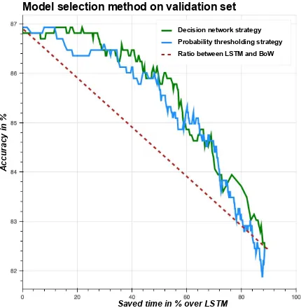
Figure 5: Model usage strategies plotted with thresholds for the probability and decision net-work strategies chosen to save a given fraction of computation time. The curve stops at around 90% savings as this represents using only the BoW model. The dashed red line represents the na¨ıve approach of using the BoW and LSTM models at random with a fixed ratio.

expensive layers. To model the compute versus accuracy tradeoff they use a test-time modifiable loss function that resembles our probability strat-egy. The composer model, similar to our deci-sion network, is not restrained to the binary choice of two models. Further, their model, similar to our decision network, does not have the draw-backs of probability thresholding, which requires every model of interest to be sequentially evalu-ated. Instead, it can in theory support a multi-class setting; choosing from several networks Boluk-basi et al.(2017) similarly use probability output to choose between increasingly expensive models. They show results on ImageNet (Deng et al.,2009) and provides encouraging time-savings with mini-mal drop in performance. This further suggest that the probability thresholding strategy is a viable al-ternative to exclusively using SoTA models. 4 Results

4.1 Model setup

Stan-Strategy Validation AUC Test AUC

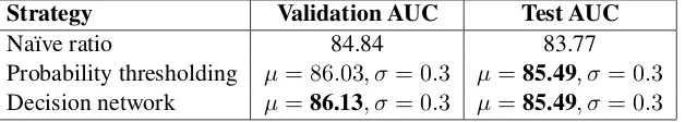
Na¨ıve ratio 84.84 83.77

Probability thresholding µ= 86.03, σ= 0.3 µ=85.49, σ= 0.3

Decision network µ=86.13, σ= 0.3 µ=85.49, σ= 0.3

Table 3: Results for each decision strategy. The AUC is the mean value of the curve from5. Each model is trained ten times with different initialization, and results are reported as mean and standard deviation over the ten runs.

ford Sentiment Treebank (SST), where “very posi-tive” is combined with “posiposi-tive”, “very negaposi-tive” is combined with “negative” and all “neutral” ex-amples are removed.

4.2 Benchmark model

To compare the two decision strategies we eval-uate the trade-off between speed and accuracy, shown in fig. 5. Speedup is gained by using the BoW more frequently. We vary the probability threshold in both strategies and compute the frac-tion of samples dispatched to each model to cal-culate average computation time. We measure the average value of the speed-accuracy curve, a form of the area-under-the-curve (AUC) metric.

To construct a baseline we consider a na¨ıve ra-tio between the two models, i.e. letYratio be the

random variable to represent the average accuracy on an unseen sample. ThenYratiohas the following

properties:

(

Pr(Yratio=ABoW) =α

Pr(Yratio=ALSTM) = 1−α (1)

WhereAis the accuracy andα∈[0,1]is the pro-portion of data used for BoW. According to the definition of the expectation of the random vari-able, we have the expected accuracy be:

E(Yratio) =

X

Pr(Yratio=y)×y (2) =α×ABoW+ (1−α)×ALSTM (3)

We calculate the cost of our strategy and bench-mark ratio in the following manner.

Cstrategy=CBoW+ (1−α)×CLSTM (4)

Cratio=α×CBoW+ (1−α)×CLSTM (5)

WhereCis the cost. Notice that the decision net-work is not a byproduct of BoW classification and requires running a second MLP model, but for simplicity we consider the cost equivalent to the probability strategy.

4.3 Quantitative results

In fig. 5 and Table 3 we find that using either guided strategy outperforms the na¨ıve ratio bench-mark by1.72 AUC.

4.4 Qualitative results

One might ask why the decision network is per-forming equivalently to the computationally sim-ple probability thresholding technique. In 5 we have provided illustrations for qualitative analysis of why that might be the case. For example,A1

provides a t-SNE visualization of the last hidden layer in the BoW (used by both policies), from which we can assess that the probability strategy and the decision network follow similar predictive patterns. There are a few samples where the prob-abilities assigned by both strategies differ signifi-cantly; it would be interesting to inspect whether or not these have been clustered differently in the extra neural layers of the decision network. To-wards that end,A2is a t-SNE plot of the last hid-den layer of the decision network. What we hope to see is that it learns to cluster when the LSTM is correct and the BoW is incorrect. However, from the visualization it does not seem to learn the ten-dencies of the LSTM. As we base our decision net-work on the last hidden state of the BoW, which is needed to reach a good solution, the decision net-work might not be able to discriminate where the BoW could not or it might have found the local minimum of imitating BoW probabilities too com-pelling. Furthermore, learning the reasoning of the LSTM solely by observing its correctness on a slim dataset could be too weak of a signal. Co-training the models in similar fashion to (Odena et al.,2017) might have yielded better results.

5 Conclusion

neural network, can make informed decisions on the difficulty of samples and when to run an ex-pensive classifier. This allow us to save computa-tional time by only running complex classifiers on difficult sentences. In our attempts to build a more general decision network, we found that it is diffi-cult to use a weaker network to learn the behavior of a stronger one by just observing its correctness.

References

D. Amodei, R. Anubhai, E. Battenberg, C. Case, J. Casper, B. Catanzaro, J. Chen, M. Chrzanowski, A. Coates, G. Diamos, E. Elsen, J. Engel, L. Fan, C. Fougner, T. Han, A. Hannun, B. Jun, P. LeGres-ley, L. Lin, S. Narang, A. Ng, S. Ozair, R. Prenger, J. Raiman, S. Satheesh, D. Seetapun, S. Sen-gupta, Y. Wang, Z. Wang, C. Wang, B. Xiao, D. Yogatama, J. Zhan, and Z. Zhu. 2015. Deep speech 2: End-to-end speech recognition in en-glish and mandarin. CoRR abs/1512.02595. http://arxiv.org/abs/1512.02595.

D. Bahdanau, K. Cho, and Y. Bengio. 2015. Neural Machine Translation by Jointly Learning to Align and Translate. InICLR.

T. Bolukbasi, J. Wang, O. Dekel, and V. Saligrama. 2017. Adaptive neural networks for fast test-time prediction. CoRR abs/1702.07811. http://arxiv.org/abs/1702.07811.

J. Deng, W. Dong, R. Socher, L.-J. Li, K. Li, and L. Fei-Fei. 2009. ImageNet: A Large-Scale Hierarchical Image Database. InCVPR.

F. Gers, J. Schmidhuber, and F. Cummins. 2000. Learning to forget: Continual prediction with lstm.

Neural Comput.12(10):2451–2471.

A. Graves. 2012. Neural networks. InSupervised Se-quence Labelling with Recurrent Neural Networks, Springer Berlin Heidelberg, pages 15–35.

A. Graves. 2016. Adaptive computation time for re-current neural networks. CoRR abs/1603.08983. http://arxiv.org/abs/1603.08983.

K. He, X. Zhang, S. Ren, and J. Sun. 2015. Deep residual learning for image recognition. CoRR

abs/1512.03385. http://arxiv.org/abs/1512.03385. S. Hochreiter and J. Schmidhuber. 1997. Long

Short-Term Memory. Neural Computation 9(8):1735– 1780.

D. Kingma and J. Ba. 2014. Adam: A method for stochastic optimization. arXiv preprint arXiv:1412.6980.

S. Merity, C. Xiong, J. Bradbury, and R. Socher. 2016. Pointer sentinel mixture models. CoRR

abs/1609.07843. http://arxiv.org/abs/1609.07843.

T. Mikolov, K. Chen, G. Corrado, and J. Dean. 2013. Efficient Estimation of Word Representations in Vector Space. InICLR (workshop).

A. Odena, D. Lawson, and C. Olah. 2017. Chang-ing model behavior at test-time usChang-ing reinforcement learning.arXiv preprint arXiv:1702.07780. J. Pennington, R. Socher, and C. D. Manning. 2014.

Glove: Global vectors for word representation. In

EMNLP.

D. Ruck, S. Rogers, M. Kabrisky, M. Oxley, and B. Suter. 1990. The multilayer perceptron as an ap-proximation to a bayes optimal discriminant func-tion. Neural Networks, IEEE Transactions on

1(4):296–298.

M. Schuster and K. Paliwal. 1997. Bidirectional re-current neural networks. Signal Processing, IEEE Transactions.

N. Shazeer, A. Mirhoseini, K. Maziarz, A. Davis, Q. Le, G. Hinton, and J. Dean. 2017. Outrageously large neural networks: The sparsely-gated mixture-of-experts layer. CoRRabs/1701.06538.

D. Silver, A. Huang, C. Maddison, A. Guez, L. Sifre, G. van den Driessche, J. Schrittwieser, I. Antonoglou, V. Panneershelvam, M. Lanctot, S. Dieleman, D. Grewe, J. Nham, N. Kalch-brenner, I. Sutskever, T. Lillicrap, M. Leach, K. Kavukcuoglu, T. Graepel, and D. Hassabis. 2016. Mastering the game of Go with deep neural net-works and tree search. Nature529(7587):484–489. https://doi.org/10.1038/nature16961.

R. Socher, A. Perelygin, J. Wu, J. Chuang, C. Manning, A. Ng, and C. Potts. 2013. Recursive deep models for semantic compositionality over a sentiment tree-bank. InEMNLP.

N. Srivastava, G. Hinton, A. Krizhevsky, I. Sutskever, and R. Salakhutdinov. 2014. Dropout: a simple way to prevent neural networks from overfitting. Journal of Machine Learning Research15(1):1929–1958. L. van der Maaten and G. Hinton. 2008. Visualizing

data using t-sne. Journal of Machine Learning Re-search9(Nov):2579–2605.

Supplementary material

Visualizations

t-SNE plots for the qualitative analysis section.

t-SNE BoW with probability outputs

Very confident Confident Doubtful Very doubtful

(a) Probability

t-SNE BoW with decision network labels

BoW LSTM

(b) Decision Network

Figure A1: t-SNE plot of the last hidden layer of the BoW model. The probabilities are colored by the confidence of the probability strategy. The colors in the decision network plot are the predictions of which model should be used at a given threshold of the decision network.

Model training

All models are optimized with Adam (Kingma and Ba,2014) with a learning rate of5×10−4_{. We train}

our models with early stopping based on maximizing accuracy of all models, except the decision network where we maximize the AUC as described in section4.2. We use SST subtrees in both the model and decision train splits and for training both models.

Model illustration: The bag of words (BoW)

As shown in fig. A3, the BoW model’s embeddings are initialized with pretrained GloVe (Pennington et al.,2014) vectors, then updated during training. The embeddings are followed by an average-pooling layer (Mikolov et al.,2013) and a two layer MLP (Ruck et al.,1990) with dropout ofp= 0.5(Srivastava et al., 2014). The network is first trained on the model train dataset (80% of training data, as shown in fig.4) until convergence (early stopping, at max 50 epochs) and afterwards on the full train dataset (100% of training data) until convergence (early stopping, at max 50 epochs).

Model illustration: The LSTM

t-SNE decision network with BoW vs LSTM comparison

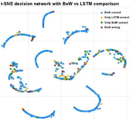
Only LSTM correct

Only BoW correct

Both wrong Both correct

Figure A2: We compare the predictions of the BoW and the LSTM to assess when one might be more correct than the other. We train the decision network to separate the yellows (only LSTM correct) from the rest. This plot enables us to evaluate if the model is able to learn the relationship between the correctness of the two models, even though it only has access to the BoW model.

Model illustration: The Decision Network

The decision network is pictured in fig.A4, it inherits all but the output layer of the BoW model trained on the model train dataset, without dropouts. The layers originating from the BoW are not updated during training. We find that it overfits if we allow such. From the last hidden layer of the BoW model, a two layer MLP (Ruck et al.,1990) with dropout ofp= 0.5(Srivastava et al.,2014) is applied on top.

(a) LSTM (b) Bag of words

Figure A3: Visualization of the BoW and LSTM model. Green refers to initialization by GloVe and updating during training. Grey is randomly initialized and updated during training. Turquoise means fixed GloVe vectors.