Adaptive fuzzy control for coordinated multiple robots with constraint using impedance learning

(1)

Adaptive Fuzzy Control for Coordinated Multiple

Robots with Constraint Using Impedance Learning

Linghuan Kong, Wei He,

Senior Member, IEEE,

Chenguang Yang,

Senior Member, IEEE,

Zhijun Li,

Senior

Member, IEEE,

and Changyin Sun

Abstract—In this paper, we investigate fuzzy neural network (FNN) control using impedance learning for coordinated multiple constrained robots carrying a common object in the presence of the unknown robotic dynamics and the unknown environment with which the robot comes into contact. Firstly, a FNN learning algorithm is developed to identify the unknown plant model. Secondly, impedance learning is introduced to regulate the con-trol input in order to improve the environment-robot interaction, and the robot can track the desired trajectory generated by impedance learning. Thirdly, in light of the condition requiring the robot to move in a finite space or to move at a limited velocity in a finite space, the algorithm based on the position constraint and the velocity constraint are proposed, respectively. To guarantee the position constraint and the velocity constraint, Integral Barrier Lyapunov function (IBLF) is introduced to avoid the violation of the constraint. According to Lyapunov’s stability theory, it can be proved that the tracking errors are uniformly bounded ultimately. At last, Some simulation examples are carried out to verify the effectiveness of the designed control.

Index Terms—Fuzzy Systems, Neural Networks, Multiple Robots, Adaptive Control, Time-varying Constraint, Impedance Learning

I. INTRODUCTION

I

N recent years, robots have been widely used in medicine [1]–[3], aerospace [4], [5] and marine vessel [6], [7], etc. As the complexity of the task and the demand of control accuracy increase, single robot hardly meet the mission re-quirement. Multiple robots can complete some tasks which are impossible for a robot. When an object is carried, multiple robots would present a large advantage over a robot in carry velocity and object weight. For example, in tool using tasks such as screwing, distribution of motions and forces required by the tasks between the multiple robot arms greatly reduces

Manuscript received November 3, 2017; revised March 16, 2018; accepted May 3, 2018. This work was supported in part by the National Natural Science Foundation of China under Grant 61522302, Grant 61573147, Grant 61625303, Grant 61751310, and Grant U1713209, in part by the National Basic Research Program of China (973 Program) under Grant 2014CB744206, in part by Anhui Science and Technology Major Program under Grant 17030901029, and in part by the Fundamental Research Funds for the China Central Universities of USTB under Grant FRF-BD-17-002A. This paper was recommended by Associate Editor C.-F. Juang. (Corresponding author: Wei He.)

L. Kong and W. He are with the School of Automation and Electrical Engi-neering, University of Science and Technology Beijing, Beijing 100083, Chi-na, and also with the Institute of Artificial Intelligence, University of Science and Technology Beijing, Beijing 100083, China. (Email: [email protected])

C. Yang was with the Zienkiewicz Centre for Computational Engineering, Swansea University, Swansea SA1 8EN, U.K. He is now with Bristol Robotics Laboratory, University of the West of England, Bristol, BS16 1QY, U.K.

Z. Li is with the Department of Automation, University of Science and Technology of China, Hefei 230026, China.

C. Sun is with School of Automation, Southeast University, Nanjing 210096, China.

the complexity and energy cost of manipulation. Therefore, research on coordinated control of multiple robots would be significant [8]. In robot applications, robot control must be subject to uncertain constraints. The violation of these con-straints leads to undesired performances such as performance degradation, hazards or system damages. And the structure of each robot is often different and there exist unmodeled dynamics and unknown parameters, accurate control of such a complicated system is difficult to obtain. However, when working in a limited environment, the robot often comes in contact with the unknown environment which is often difficult to describe in a nonlinear model, and an interaction force develops between the robot and its environment. Therefore, the main difficulty of controlling those systems lies in the fact that, when the robot encounters unknown environments, the interaction force and the position of the robot, must be controlled collaboratively. In this paper, we would analyse coordinated control problems of multiple robots with time-varying constraints in the present of the unknown environment and unmodeled dynamics and design adaptive fuzzy neural network control for coordinated control of multiple robots in a finite task space.

(2)

neural networks are used to identity the unknown plant of an environment-robot system, and the fuzzy algorithm can improve the interaction between the robot and its environment. In [37], fuzzy neural networks are used to approximate the unknown nonlinear plant of nonlinear systems. In [38], an adaptive fuzzy neural network control scheme is proposed for a marine, and the fuzzy policy can ensure that the tracking error converges to an arbitrarily small region near zero in a finite time.

Recently, the tracking control for nonlinear systems is investigated, motivated by the fact that practical systems are subjected to constraint [39] in the form of mechani-cal structure, safety specifications and physics performance. These constraints include input constraint [40]–[45], output constraint [46]–[48] and full-state constraint [49]–[51]. An appropriate controller sometimes makes the index of a sys-tem remain the corresponding constraint region in order to obtain an approximation optimal performance. In [52], it has been proved that log-type Barrier Lyapunov functions can guarantee the constraint. In [53], log-type Barrier Lyapunov function is introduced to guarantee the full-states remain in the predefined constraint region. However, the abovelog-type Barrier Lyapunov function constraint technique may make the corresponding variables go beyond the constraint region when the size of the vibration is too large or initial values are too large, which may lead to system impairments or even system failures. In [54], Integral Barrier Lyapunov function (IBLF) can compensate the effect of constraint and avoid the violation of states without the requirement of initial values, except that when initial values are demanded to satisfy the constraint. However, log-type Barrier Lyapunov function introduced in [52], [53], [55] just constrains error signals, therefore, an ad-ditional mapping to the state space is needed. Integral Barrier Lyapunov functions introduced in [56] directly constrain state signals without an additional mapping, and initial states are relaxed to whole constrained space. In [55], log-type Barrier Lyapunov functions are used to avoid the violation of the varying constraint for a constrained robot. The time-varying constraint is more general than the constant constraint introduced in [52].

Position control methods give adequate performances for an uncertain robot, and only require the robotic end-effector to track a desired trajectory in free space. But, when the robot comes in contact with the environment, it is inevitable that an interaction force would develop between the robot and its environment. Research studies then focus on how to regulate the robot-environment interaction. Hogan first presents impedance control theory to regulate the interaction between the robotic end-effector and the force exerted on the environment. [57] thinks the learning capability can regular the interaction between the robot and its environment. In [58], two impedance control algorithms that generate a desired dynamics of the robot with environment are developed for robotic manipulators. However, the results mentioned in [57]– [59] assume that robot dynamics is known. In [60], adaptive impedance learning control is proposed for a human-robot system in the presence of unknown robotic dynamics.

This paper would handle coordinated control problems of multiple robots with time-varying constraints, in the present

of the unknown environment with which the robot comes into contact. Impedance learning is employed to improve the environment-robot interaction, fuzzy neural networks are constructed to approximate the unknown robotic dynamics, and time-varying constraints guarantee a satisfactory tracking performance by ensuring that the system states remain in a small neighborhood of the reference signal, such that the fuzzy neural network control algorithm is formed. This type of the control algorithm is suitable for the environment-robot interaction control and objection manipulation. This paper is an extended work from the previous works [26], [36]. In [36], only single robot with the constant constraint is considered for the environment-robot interaction without involving co-ordinated control of multiple robots. But in most situations, multiple robots with the time-varying constraint would present a large advantage over a robot with the constant constraint in the movement velocity and the carried weight. Further, in [26], coordinated control of two robots is investigated without considering the time-varying constraint. Consequently, our work can be considered as the improvement of [26], [36]. Fuzzy neural networks combine advantages of both fuzzy systems and neural networks, and have fewer adjustable parameters and can reduce online computation load. Thus fuzzy neural network control can satisfy the requirement of real-time control better with fewer time consuming.

The main contributions of this paper are summarized as follows: 1) Compared with the conventional Lyapunov func-tions includinglog-type [55] andtan-type [36], integral barrier Lyapunov functions are developed to constrain state signals directly, rather than error signals, with avoiding carrying out an additional mapping to the state space. Therefore, the initial states can be relaxed to whole constrained space. 2) An learning algorithm based on FNN structure is proposed, which needs no previous information of the system. The unknown system plant is approximated by structuring an appropriate FNN structure. 3) The time-varying output constraint and the time-varying full-state constraint are considered, respectively. The time-varying constraint is more general and complicated than constant constraint. Based on the time-varying constraint, the designed algorithm has a wider application range. 4) Impedance learning is introduced to improve the interaction between the robot and the unknown environment.

Notations 1: Let λmin(•) and λmax(•) denote the

min-imum and maxmin-imum eigenvalues of matrix •, respective-ly. Let ∥ · ∥ be the Euclidean norm of a vector. Let blockdiag[A1, A2, . . . , An] denote a diagonal block matrix,

where Ai, i = 1, . . . , n, is a matrix. Let sgn(·) be a sign function, where

sgn(·) =

{

1, · ≥0

−1, ·<0 (1)

II. PRELIMINARIES ANDPROBLEMFORMULATION

A. System Description

(3)

x y z

xo

Fe

xo

o

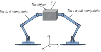
The first manipulator The second manipulator

[image:3.612.93.257.53.138.2]

The object

Fig. 1. Coordinated control of two robotic manipulators

environment dynamics and that there exist unmodeled plants and unknown parameters in the robot model. Butmrobots are demanded to carry an object in a coordinated way in a finite space. Therefore, the main problems are to tackle the unknown dynamics and unknown parameters of the robotic model, the interaction between the robot and its unknown environment, and the time-varying constraint. The kinetic equation of ith manipulator [26] in joint space is expressed as

Di(qi)¨qi+Ci(qi,q˙i) ˙qi+Gi(qi) =τi−JiT(qi)τei

i= 1, . . . , m (2)

where qi ∈ Rn _{is the vector of joint variable,} _Di₍_qi₎ _∈

Rn×n _{denotes the positive definite joint quality inertia matrix,} Ci(qi,qi˙)∈ Rn×n denotes the joint Coriolis and centrifugal matrix, Gi(qi)denotes the joint gravitational forces, τi ∈Rn

denotes the control input vector, Ji(qi) ∈Rn×n denotes the Jacobian matrix, τei∈Rn denotes the force from the object.

Based on (2), the kinetic equation ofm robots is given by

Dx(q)¨q+Cx(q,q˙) ˙q+Gx(q) =τ−JT(q)τe (3)

where q = [qT

1, . . . , qTm]T ∈ Rmn; τ =

[τT

1, . . . , τmT]T ∈ Rmn; τe = [τeT1, . . . , τemT ]T ∈ Rmn; Dx(q) = blockdiag[D1(q1), . . . , Dm(qn)] ∈ Rmn×mn; Cx(q,q˙) = blockdiag[C1(q1,q˙1), . . . , Cm(qm,q˙m)] ∈

Rmn×mn_; _G

x(q) = [GT1(q1), . . . , GTm(qm)]T ∈ Rmn; J(q) = blockdiag[J1(q1), . . . , Jm(qm)]∈Rmn×mn.

Let xo ∈ Rn _{denote the position/orientation vector of the}

object. The motion of the object is driven by the force vector

τo∈Rn_and_τd_∈_Rn _{acting on the center of mass the object,}

whereτodenotes the resultant force vector frommrobots and

τd denotes the force vector from the unknown environment. The kinetic equation [26] of the object is given by

Mo(xo)¨xo+Co(xo,xo˙ ) ˙xo+Go(xo) =τo−τd (4)

and Mo(xo)∈Rn×n is a symmetric positive definite inertial matrix, Co(xo,xo˙ ) ∈ Rn×n is a corioli and centrifugal matrix, Go(xo) ∈ Rn is the gravitational force vector. Let

xi, i= 1, . . . , m, denote the position/oritations of ith robot’s end-effector in the Cartesian space. According to [61], the relationship betweenxi andqi is given by

˙

xi =Ji(qi) ˙qi (5)

The relationship [8] betweenx˙i andx˙o is given by

˙

xi=Jio(xo) ˙xo (6)

where Jio(xo) denotes the Jacobian matrix from the object

frame to the ith robot’s end-effector. By combining (5) and (6), the relationship between the joint velocity of the ith

manipulator and the velocity of the object is obtained by

Ji(qi) ˙qi=Jio(xo) ˙xo (7)

Assume that robots work in a nonsingular region, thus the inverse of the Jacobian matrix Ji(qi) exists. Considering all

the manipulators acting on the object at the same time, yields

˙

q=J−1(q)Jo(xo) ˙xo (8)

¨

q= d

dt(J −1

(q)Jo(xo)) ˙xo+J−1(q)Jo(xo)¨xo (9)

whereJo(xo) = [J1To(xo), . . . , JmoT (mo)]T. After substituting

(8) and (9) into (3) and then adding (4), the kinetic equation of m coordinated multiple robots with object motion (4) in Cartesian space is given by

M(q)¨xo+C(q,q˙) ˙xo+G(q) =Fo−Fe (10)

where

M(q) =J_oT(xo)J−T(q)Dx(q)J−1(q)Jo(xo) +Mo(xo)

C(q,q˙) =JoT(xo)J−T(q)Dx(q) d dt(J

−1₍_q₎_Jo₍_xo₎₎

+J_oT(xo)J−T(q)Cx(q,q˙)J−1(q)Jo(xo) +Co(xo,xo˙ )

G(q) =J_oT(xo)J−T(q)Gx(q) +G(xo)

Fo=J_oT(xo)J−T(q)τ, Fe=τd

For the convenience, in the subsequent design,M, C, Gdenote

M(q), C(q,q˙), G(q), respectively.

The system state xo = [xo1, . . . , xon]T is commanded to

satisfy the following constraint

|xoi|< kci, |x˙oi|< kdi, i= 1, . . . , n (11)

where kci, kdi are positive time-varying functions, given the

initial states satisfy |xoi(0)|< kci(0),|x˙oi(0)|< kdi(0). The

full-state constraint is denoted as the set {xo ∈ Rn_||_xoi| _< kci,|xoi|˙ < kdi, i = 1, . . . , n}. The output constraint is denoted as the set {xo∈Rn_||_xoi|_{< kci, i}_{= 1}_{, . . . , n}_}_.

In real robotic systems, the object usually suffers from force from environment when moving in task space. The impedance dynamics betweenFe andeis given by

Mde¨+Cde˙+Gde=Fe (12)

whereMd, Cd, Gdare defined by the user. Impedance error e

originates from forceFe. Let us definee=xd−xc, wherexc

is the desired trajectory, xd is the commanded trajectory the users define, which is bounded and twice differentiable. It can be known from (12) that impedance erroreis equal to zero if

Feis equal to zero. Substitutinge=xd−xc into (12), yields

Mdxc¨ +Cdxc˙ +Gdxc =Mdxd¨ +Cdxd˙ +Gdxd−Fe (13)

According to (13), the impedance control objective can be achieved. It should be noted that (13) may be interpreted as a simply filter and xc is obtained online ifxd, Md, Cd, Gd and the forceFe are given.

B. Fuzzy Neural Networks

(4)

fuzzy rules, and the defuzzifier [62]. Consider l fuzzy IF-THEN rules R(k)_{: If} _x

1 is Ak1 and · · · and xn is Akn, then

y is Wk_{, k} _{= 1}_,_{· · ·} _{, l}_{, where} _R(k) _{denotes the} _k_{-th rule,}

1 ≤ k ≤ l,(x1, x2,· · ·, xn)T ∈ U ⊂ Rn, and y ∈ R are

the linguistic variables that are associated with the inputs and output of the fuzzy logic system, respectively, and Ak

i and Wk_{denote the fuzzy sets in}_U_and_R_{. The fuzzy logic system}

performs a nonlinear mapping fromUtoR. In this paper, the fuzzy logic system is

y(x) =

∑l

k=1yk(Πni=1µAk i(xi)) ∑l

k=1(Πni=1µAk i(xi))

(14)

where x = [x1, x2,· · ·, xn]T and µAk

i(xi) is the mem-bership function of linguistic variable xi with µ_Ak

i(xi) =

exp[−(xi−c2ik)

σ2

ik

]. For clarify, the weight vector and fuzzy basis function vector are defined, respectively, as θ =

[y1, y2,· · ·, yl]T and ϕ(x, c, σ) = [s1, s2,· · ·, sl]T, where

sk = ∏n

i=1µAk_i(xi)

[∑l k=1

∏n

i=1µAk_i(xi)], c = [c

T

1, cT2,· · ·, cTn]T and σ =

[σ1T, σ2T,· · ·, σnT]T. Therefore, (14) can be represented as

y=θTϕ(x, c, σ) (15)

It has been proven that the fuzzy logic system (15) has the capacity to approximate any given real continuous functions over a compact set to any degree of accuracy. Therefore, we have the following approximation for the unknown nonlinear functionfi(xi),i= 1,2,· · · , n.

fi(xi) =θi∗Tϕ(xi) +ϵi (16)

where θ∗T

i is an unknown constant parameter vector, ϕ(xi)

is the fuzzy basis function and ϵi is the approximation error,

which satisfiesmaxZ∈ΩZ||ϵi||< ϵ∗i, whereϵ∗i >0is unknown

bound [63].

C. Preliminaries

To guarantee the time-varying constraint, we introduce the integral barrier Lyapunov function [64] as

V =

n

∑

i=1

∫ zi

0

σk2 ci k2

ci−(σ+αi)2

dσ (17)

where i = 1, . . . , n, zi = xi−αi, and αi is a continuously differentiable function satisfying |αi|< kci, i= 1, . . . , n. It is known thatV is a continuously positive differentiable function over the set {|xi|< kci}.

Lemma 1: (17) is a continuously positive differentiable function over the set {|xi| < kci}. As for |xi| < kci, i = 1, . . . , n, there is

z2 i

2 ≤V ≤

k2 cizi2 k2

ci−x 2 i

(18)

Proof: See the Appendix.

Remark 1: In (17), kci is a time-varying function and denotes the constrained upper bound ofxi, namelysup|xi|< kci, for∀t >0, given that initial value|xi(0)|< kci(0).

III. CONTROL DESIGN

For the robotic dynamics (10), it is tough to design a control policy to cope with the effect of time-varying constraints in the

Impedance model ¦ - 2 Fo

z

Carried object Constrained robots

FNNs

1

z

2

z

Updating law

1

z

2 z

- 1

z

d x

c x

1

x

2

x

e

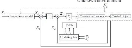
[image:4.612.323.548.56.138.2]

F Unknown environment

Fig. 2. System structure

presence of unknown environment. The problem is especially complex to solve full-state time-varying constraints. In this paper, the control schemes are proposed for the full-state time-varying constraint and the output time-varying constraint, respectively. Fig. 2 shows the system structure. To facilitate the control design, we define x1=xo, x2= ˙xo. The kinetic

equation (10) can be rewritten as

˙

x1=x2

˙

x2=M−1(Fo−Fe−G−Cx2) (19)

wherex1= [x11, . . . , x1n]T,x2= [x21, . . . , x2n]T. The error

variables are defined as follows

z1=x1−xc

z2=x2−α (20)

where z1 = [z11, . . . , z1n]T, z2 = [z21, . . . , z2n]T, xc =

[xc1, . . . , xcn]T,α= [α1, . . . , αn]T is a virtual control aiming

to make tracking errorz1converge to a small region near zero.

A. Control Design with Output Constraint

In this section, system output x1 should be demanded to

be constrained by time-varying function kci ∈ R+, namely

|x1i|< kci,i= 1, . . . , n. To ensure this constraint, an integral

barrier Lyapunov function is constructed as

V1= n

∑

i=1

∫ z1i

0

σk2 ci k2

ci−(σ+xci)2

dσ (21)

The derivative of (21), with regard to time, is

˙

V1= n

∑

i=1 ∂V1 ∂z1i

dz1i

dt +

n

∑

i=1 ∂V1 ∂xci

dxci

dt +

n

∑

i=1 ∂V1 ∂kci

dkci dt

=

n

∑

i=1 k2

ciz1i k2

ci−x21i

(z2i+αi−x˙ci)

+

n

∑

i=1 z1i(

k2 ci k2

ci−x21i

−ρi) ˙xci+

n

∑

i=1 ∂V1 ∂kci

dkci

dt (22)

where

rhoi = kci 2z1i

ln(kci+z1i+xci)(kci−xci) (kci−z1i−xci)(kci+xci)

(23)

Then, virtual controlαi, i= 1, . . . , n, is designed as

αi=−kiz1i+

(k2

ci−x21i) ˙xciρi k2

ci

−k2ci−x21i

k2 ciz1i

∂V1 ∂kci

dkci dt (24)

(5)

Take virtual control αinto (22), we further have

˙

V1=− n

∑

i=1

kik2_ciz₁2_i k2

ci−x21i

+

n

∑

i=1

k_ci2z1iz2i k2

ci−x21i

(25)

An integral barrier Lyapunov function is constructed as

V2=V1+

1 2z

T

2M z2 (26)

Design the control input F_o∗ as

Fo∗=−

    

k2_c₁z11

k2

c1−x211 .. .

k2

cnz1n

k2

cn−x21n    

−K2z2+Fe+G+Cα+Mα˙

(27)

Substituting (24) and (27) into the time derivative of (26), we have

˙

V2=− n

∑

i=1

kik2ciz12i k2

ci−x21i

−z₂TK2z2

≤ − n

∑

i=1

∫ z1i

0

σkik_ci2 k2

ci−(σ+xci)2

dσ−z2TK2z2

≤ −κ2V2 (28)

where κ2 = min{ min 1≤i≤n(ki),

2λmin(K2)

λmax(M)}. To ensure κ2 > 0, parameters should satisfy min

1_≤i_≤n(ki) > 0,

λmin(K2)

λmax(M) > 0.

V2 will converge into a small range near zero with the

convergence ratee−κ2_{. But there are uncertainties in}_{G, C, M}_, thereforeF_o∗cannot be obtained in a real system. Fuzzy neural networks are used to approximate the uncertainties inG, C, M. An adaptive fuzzy neural network controller is designed as

Fo=−

    

k2

c1z11

k2

c1−x211 .. .

k_cn2 z1n

k2

cn−x21n    

−K2z2+Fe+ ˆθGTϕG(ZG)

+ ˆθT_CϕC(ZC)α+ ˆθMT ϕM(ZM) ˙α+Krsgn(z2) (29)

where Kr = diag[kr1, . . . , krn] > 0; θˆG,θˆC,θˆM are

ac-tual weight vectors, θ∗_G, θ_C∗, θ_M∗ are optimal weight vectors, ˜

θG = ˆθG −θ∗_G,θC˜ = ˆθC−θ_C∗,θM˜ = ˆθM −θ∗_M are error weight vectors, ZG= [xT1, xT2]T, ZC= [xT1, xT2, αT]T, ZM =

[xT

1, xT2, αT,α˙T]T are fuzzy neural network inputs,

respective-ly.

To improve the system control performance, we design the updating laws as

˙ˆ

θGi=−ΓGi(ϕGi(ZG)z2i+σGθGiˆ ) (30)

˙ˆ

θCi=−ΓCi(ϕCi(ZC)z2iαi+σCθCiˆ ) (31)

˙ˆ

θM i=−ΓM i(ϕM i(ZM)z2iα˙i+σMθˆM i) (32)

whereΓGi,ΓCi,ΓM iare positive definite symmetric matrixes, σG, σC, σM are positive constants, θˆGTϕG,θˆTCϕC,θˆTMϕM are

estimated values ofθ∗T

G ϕG, θ∗CTϕC, θM∗TϕM, respectively.

θ∗_GTϕG=G+ϵG (33)

θ∗_CTϕC=C+ϵC (34)

θ∗MTϕM =M+ϵM (35)

whereϵG, ϵC, ϵM are approximation errors satisfying||ϵG|| ≤ ¯

ϵG,||ϵC|| ≤ ¯ϵC,||ϵM|| ≤ ϵM¯ , with ¯ϵG,¯ϵC,¯ϵM being positive constants.

Choose a positive Lyapunov function as

V3= n

∑

i=1

∫ z1i

0

σk2 ci k2

ci−(σ+xdi)2 dσ+1

2z

T

2M z2

+1 2

n

∑

i=1

˜

θ_GiT Γ−_Gi1θ˜Gi+

1 2

n

∑

i=1

˜

θ_CiT Γ−_Ci1θ˜Ci

+1 2

n

∑

i=1

˜

θ_{M i}T Γ−_{M i}1θM i˜ (36)

Substituting (24) and (29) into the time derivative of (36), we have

˙

V3=− n

∑

i=1 kik2

ciz12i k2

ci−x 2 1i

−z₂TK2z2+zT2(˜θ

T

GϕG(ZG)

+ ˜θTCϕC(ZC) + ˜θTMϕM(ZM)−ϵG−ϵCα−ϵMα˙

+Krsgn(z2)) + n

∑

i=1

˜

θT_GiΓ−_Gi1θGi˙ˆ +

n

∑

i=1

˜

θ_CiT Γ−_Ci1θCi˙ˆ

+

n

∑

i=1

˜

θT_{M i}Γ−_{M i}1θ˙ˆM i (37)

Let us define(ϵG+ϵCα+ϵMα˙)i asEi, i= 1, . . . , n,for the

interval t ∈ [0,+∞), where (·)i is i-th element of a vector.

Therefore, we obtainE= [E1, . . . , En]T.

Substituting the weight updating laws into (37), we have

˙

V3=− n

∑

i=1

kikci2z12i k2

ci−x21i

−zT₂K2z2+z2T(Krsgn(z2)−E)

+z₂T(˜θT_GϕG(ZG) + ˜θ_CTϕC(ZC)α+ ˜θT_MϕM(ZM) ˙α)

− n

∑

i=1

˜

θ_GiT (ϕGi(ZG)z2i+σGθˆGi)

− n

∑

i=1

˜

θ_CiT (ϕCi(ZC)z2iαi+σCθCiˆ )

− n

∑

i=1

˜

θ_{M i}T (ϕM i(ZM)z2iαi˙ +σMθM iˆ ) (38)

Notice that

z₂Tθ˜T_GϕG(ZG) = n

∑

i=1

˜

θT_GiϕGi(ZG)z2i (39)

z2Tθ˜TCϕC(ZC)α= n

∑

i=1

˜

θTCiϕCi(ZC)z2iαi (40)

z₂Tθ˜T_MϕM(ZM) ˙α=

n

∑

i=1

˜

θ_{M i}T ϕM i(ZM)z2iαi˙ (41)

(6)

we have zT

2(Krsgn(z2)−E)≤0, therefore

˙

V3≤ − n

∑

i=1

kik2_ciz₁2_i k2

ci−x21i

−z₂TK2z2−

n

∑

i=1

˜

θT_GiσGθGiˆ

− n

∑

i=1

˜

θT_CiσCθCiˆ − n

∑

i=1

˜

θ_{M i}T σMθM iˆ (42)

Since −∑n_i₌₁θ˜T_GiσGiθGiˆ ≤ −σGi

2

∑n i=1θ˜

T

GiθGi˜ + σGi

2

∑n i=1θ∗

T GiθGi∗ ,−

∑n i=1θ˜

T

CiσCiθCiˆ ≤ − σCi

2

∑n i=1θ˜

T CiθCi˜

+ σCi

2

∑n i=1θ∗

T

Ciθ∗Ci and −

∑n i=1θ˜

T

M iσM iθM iˆ ≤

−σM i

2

∑n i=1θ˜

T M iθM i˜ +

σM i

2

∑n i=1θ∗

T

M iθ∗M i, we have

˙

V3≤ − n

∑

i=1

kik2ciz12i k2

ci−x21i

−σGi

2

n

∑

i=1

˜

θTGiθGi˜ − σCi 2 n ∑ i=1 ˜

θCiT θCi˜

−σM i

2

n

∑

i=1

˜

θT_{M i}θM i˜ +σGi 2

n

∑

i=1

θ_Gi∗Tθ_Gi∗ −zT₂K2z2

+σCi 2

n

∑

i=1

θ∗_CiTθ∗_Ci+σM i 2

n

∑

i=1

θ∗_{M i}Tθ∗_{M i}

≤ −κ3V3+C3 (43)

where

κ3= min{k1, . . . , kn,

2λmin(K2) λmax(M)

, σGi

λmax(Γ−Gi1)

, σCi

λmax(Γ−Ci1) ,

σM i λmax(Γ−M i1)

}

C3= σGi

2

n

∑

i=1

θ_Gi∗Tθ_Gi∗ +σCi 2

n

∑

i=1

θ∗_CiTθ∗_Ci+σM i 2

n

∑

i=1

θ_{M i}∗Tθ∗_{M i}

To ensureκ3>0, C3>0, controller parameters should satisfy ki >0,λmax(K2)>0,σGi>0,σCi>0 andσM i>0,i=

1, . . . , n. Therefore, we know thatV3 is bounded for∀t >0.

Theorem 1: For the robot system (10) with output time-varying constraint, and FNN control (29) with updating law (31)-(33) and impedance learning (13), given that initial con-ditions are bounded. It can be concluded that target impedance is achieved and the tracking errors are uniformly bounded ultimately. The tracking errors converge to a small range near zero and the range can be changed by choosing appropriate parameters. The system output is constrained by the predefined constraint region the user defines. The tracking error z1

converges to the compact set Ωz1 := {z1 ∈ Rn||z1i| ≤ √

2B, i = 1, . . . , n}. The tracking error z2 converges to the

compact set Ωz2 := {z2 ∈ Rn||z2i| ≤ √

2B, i = 1, . . . , n}, whereB:=V3(0) +C_κ3

3.

B. Control Design with Full-State Constraint

The FNN control with the full-state constraint will be presented in this section. It should be emphasized that although the control design is similar to the control (29), the system states should be demanded to be constrained by the time-varying constraint in the control design. In this sense, the system state x2 should be constrained satisfying |x2i| ≤ kdi

for ∀t >0 wherekdi ∈R+, i = 1, . . . , n, is a time-varying

function. The detailed design is presented as follows. To ensure that system states remain in the predefined constraint region,

a positive integral barrier Lyapunov function is constructed as

V5=V2+V4 (44)

where

V4= n

∑

i=1

∫ z2i

0

σk2 di

k_di2 −(σ+αi)2dσ (45)

The derivative ofV5, with respect to time, is

˙

V5= ˙V2+ n

∑

i=1 ∂V4 ∂z2i

dz2i

dt + n ∑ i=1 ∂V4 ∂αi dαi dt + n ∑ i=1 ∂V4 ∂kdi dkdi dt

= ˙V2+ n

∑

i=1 k2

diz2iz˙2i k2

di−x 2 2i + n ∑ i=1 z2i(

k2 di k2

di−x 2 2i

−ρ2i) ˙αi

+ n ∑ i=1 ∂V4 ∂kdi dkdi dt (46) where

ρ2i= kdi

2z2i

ln(kdi+z2i+αi)(kdi−αi) (kdi−z2i−αi)(kdi+αi)

(47)

The model-based controller is designed as

F_o∗=−

     k2

c1z11

k2

c1−x211 .. .

k2_cnz2₁_n kcn−x21n

    −     

k2_d₁k11z21

k2

d1−x 2 21 .. .

k_dn2 k1nz2n

k2

dn−x22n      −     

( k2d1

k2

d1−x 2 21 −

ρ21) ˙α1

.. .

( k2dn

k2

dn−x

2 2n −

ρ2n) ˙αn

    − n ∑ i=1 1

z2i ∂V4 ∂kdi

dkdi dt

−K2z2+Fe+G+Cα+Mα˙ (48)

wherek1i, i= 1, . . . , n,is a positive constant.

Substituting (24) and (48) into (46), we have

˙

V5=− n

∑

i=1

kik2ciz21i k2

ci−x21i −

n

∑

i=1 k1ikdi2z

2 2i k2

di−x22i

+

n

∑

i=1 k2

diz2iz˙2i k2

di−x22i

−zT2K2z2≤ −κ5V5+

n

∑

i=1

k2_diz2iz˙2i k2

di−x 2 2i

(49)

where

κ5= min{ min

1_≤i_≤nki,1min_≤i_≤nk1i,

2λmin(K2) λmax(M) }

(50)

Multiplying (49) byeκ5t_yields

eκ5t_V˙

5≤ −κ5eκ5tV5+eκ5tg(t)N(z2) ˙z2 (51)

whereg(t) = diag[ k2d1

(k2

d1−x221) cos(π2z21),· · ·,

k2_dn (k2

dn−x22n) cos(π2z2n)] , N(z2) = [z21cos(π₂z21),· · ·, z2ncos(π₂z2n)]T. Integrating

(51), yields

V5(t)≤e−κ5tV5(0) +e−κ5t

∫ t

0

g(τ)N(z2) ˙z2eτ tdτ (52)

where t ∈ [0, tf). According to [36], we known that

∥∫t

0g(τ)N(z2) ˙z2e

τ t_dτ_∥ _{is bounded. Therefore, define} _N

as an upper bound of ∥∫₀tg(τ)N(z2) ˙z2eτ tdτ∥, namely

∥∫t

0g(τ)N(z2) ˙z2e

(7)

conclud-ed thatV5(t), z1, z2are bounded on[0, tf)ifκ5>0. However,

the uncertainties exist in M, C, G, F_o∗ is not available in a real system. FNNs have the ability to approximate nonlinear functions in ideal accuracy, thus in this section FNNs are used to approximateM, C, G, respectively. An adaptive FNN controller is designed as

Fo=−

     k2

c1z11

k2

c1−x211 .. .

k2

cnz1n

k2

cn−x21n     −      k2

d1k11z21

k2

d1−x221 .. .

k2

dnk1nz2n

k2

dn−x22n      −     

( k2d1

k2

d1−x221 −

ρ21) ˙α1

.. .

( k2dn

k2

dn−x22n−

ρ2n) ˙αn

    − n ∑ i=1 1

z2i ∂V4 ∂kdi

dkdi dt

−K2z2+Fe+ ˆθTGϕG(ZG) + ˆθ T

CϕC(ZC)α

+ ˆθ_MT ϕM(ZM) ˙α+Krsgn(z2) (53)

A Lyapunov function is constructed as

V6=V5+

1 2 n ∑ i=1 ˜

θ_GiT Γ−_Gi1θGi˜ +1 2

n

∑

i=1

˜

θT_CiΓ−_Ci1θCi˜

+1 2 n ∑ i=1 ˜

θT_{M i}Γ−_{M i}1θ˜M i (54)

Substituting (24) and (53) into the time derivative of V6, we

have

˙

V6=− n

∑

i=1

kik2_ciz₁2_i k2

ci−x21i −

n

∑

i=1

k1ikdi2z 2 2i k2

di−x 2 2i + n ∑ i=1

k2_diz2iz˙2i k2

di−x 2 2i

−zT₂K2z2+z2T(˜θ

T

GϕG(ZG) + ˜θTCϕC(ZC)

+ ˜θT_MϕM(ZM)−ϵG−ϵCα−ϵMα˙ +Krsgn(z2))

+

n

∑

i=1

˜

θTGiΓ− 1 GiθGi˙ˆ +

n

∑

i=1

˜

θCiT Γ− 1 CiθCi˙ˆ

+

n

∑

i=1

˜

θT_{M i}Γ−_{M i}1θM i˙ˆ (55)

Let us define(ϵG+ϵCα+ϵMα˙)i as Ei, i= 1, . . . , n,for the

interval t ∈ [0,+∞), where (·)i is ith element of a vector.

Therefore, we obtain E = [E1, . . . , En]T. Substituting

(31)-(33) and (40)-(42) into (55), we have

˙

V6≤ − n

∑

i=1

kik2ciz12i k2

ci−x21i −

n

∑

i=1

k1ik2diz 2 2i k2

di−x22i

+

n

∑

i=1 k2

diz2iz˙2i k2

di−x22i

−z₂TK2z2+z2T(Krsgn(z2)−E)−

n

∑

i=1

˜

θT_GiσGθGiˆ

− n

∑

i=1

˜

θ_CiT σCθCiˆ − n

∑

i=1

˜

θT_{M i}σMθM iˆ (56)

The gain Kr is designed to satisfy |Ei| ≤ kri, i = 1, . . . , n,

we have zT

2(Krsgn(z2)−E)≤0. And since

− n

∑

i=1

˜

θ_GiT σGiθGiˆ ≤ −σGi

2

n

∑

i=1

˜

θ_GiT θGi˜ +σGi 2

n

∑

i=1 θ∗_GiTθ∗_Gi

− n

∑

i=1

˜

θ_CiT σCiθCiˆ ≤ −σCi

2

n

∑

i=1

˜

θ_CiT θCi˜ +σCi 2

n

∑

i=1 θ∗_CiTθ∗_Ci

− n

∑

i=1

˜

θ_{M i}T σM iθˆM i≤ − σM i

2

n

∑

i=1

˜

θ_{M i}T θ˜M i+ σM i

2

n

∑

i=1

θ∗_{M i}Tθ∗_{M i}

we have

˙

V6≤ − n

∑

i=1

kik2_ciz2₁_i k2

ci−x21i −

n

∑

i=1 k1ikdi2z

2 2i k2

di−x 2 2i + n ∑ i=1

k2_diz2iz˙2i k2

di−x 2 2i

−z₂TK2z2−

σGi 2 n ∑ i=1 ˜

θT_GiθGi˜ −σCi

2

n

∑

i=1

˜

θT_CiθCi˜

−σM i

2

n

∑

i=1

˜

θT_{M i}θ˜M i+ σGi

2

n

∑

i=1 θ∗_GiTθ∗_Gi

+σCi 2

n

∑

i=1

θ∗CiTθCi∗ + σM i

2

n

∑

i=1

θM i∗Tθ∗M i

≤ −κ6V6+C6+

n

∑

i=1

k_di2z2iz˙2i k2

di−x 2 2i

(57)

where

κ6= min{ min

1≤i≤n(ki),1min≤i≤n(k1i),

2λmin(K2) λmax(M)

, σGi

λmax(ΓGi) ,

σCi λmax(ΓCi)

, σM i

λmax(ΓM i) }

C6= σGi

2

n

∑

i=1

θ∗_GiTθ∗_Gi+σCi 2

n

∑

i=1

θ_Ci∗Tθ_Ci∗ +σM i 2

n

∑

i=1

θ∗_{M i}Tθ∗_{M i}

Multiplying (57) byeκ6t_yields

eκ6t_V˙

6≤ −κ6eκ6tV6+eκ6t C6 κ6

+eκ6t_g₍_t₎_N₍_z

2) ˙z2 (58)

whereg(t) = diag[ k2d1

(k2

d1−x 2

21) cos(π2z21),· · ·,

k2_dn (k2

dn−x

2

2n) cos(π2z2n)] , N(z2) = [z21cos(π₂z21),· · ·, z2ncos(π₂z2n)]T. Integrating

(58), yields

V6(t)≤e−κ6tV6(0) + C6 κ6

+e−κ6t

∫ t

0

g(τ)N(z2) ˙z2eτ tdτ (59)

where t ∈ [0, tf). According to [36], we known that ∥∫₀tg(τ)N(z2) ˙z2eτ tdτ∥ is bounded. Therefore,

de-fine N as an upper bound of ∥∫₀tg(τ)N(z2) ˙z2eτ tdτ∥,

namely ∥∫₀tg(τ)N(z2) ˙z2eτ tdτ∥ ≤ N . To ensure that κ6 > 0, C6 > 0, controller parameters should satisfy

min

1≤i≤n(ki) >0,1min≤i≤n(k1i) >0,

2λmin(K2)

λmax(M) >0,

σGi

λmax(ΓGi) >

0, σCi

λmax(ΓCi) >0,

σM i

λmax(ΓM i) >0. Therefore,V6 is bounded.

(8)

range near zero and the range can be changed by choosing appropriate parameters. The system states are constrained by the predefined constraint region the user defines. The tracking errorz1converges to the compact setΩz1:={z1∈Rn||z1i| ≤ √

2B1, i= 1, . . . , n}. The tracking error z2 converges to the

compact set Ωz2 :={z2 ∈Rn||z2i| ≤ √

2B1, i= 1, . . . , n},

whereB1:=V6(0) +C_κ6

6 +N .

IV. SIMULATION

X

O Y

Z

11

l

12

l

13

l

21

l

22

l

23

l

1

X

1

Y

1 Z

2 X

2

Y

2

Z

Object

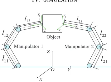
[image:8.612.87.265.169.300.2]

Manipulator 1 Manipulator 2

Fig. 3. Simulation scenario.

In this section, an environment-robot interaction system is considered to verify the effectiveness of the proposed control (29) and (53), respectively. The environment-robot interaction system includes two robots sharing the same system parame-ters and 3 degrees of freedom including three rotary degrees, an object and a force sensor located on the surface of the object as shown in Fig. 3. In Fig. 3, letmi1,mi2andmi3 denote the

mass of link 1, link 2 and link 3 of manipulator i, i= 1,2, respectively, let li1, li2 and li3 denote the length of link 1,

link 2 and link 3 of manipulator i, i= 1,2, respectively, and let Iji denote the moment of inertia of link j, j = 1,2,3,

of manipulator i, i = 1,2, with regard to an axis coming out of the page passing through the center of mass of link i. Simulation time istf = 20s. The sampling period is0.0025s.

The trajectory commanded by the user is given by

xd=

  xdxd12

xd3

 =



 0.8 + 00..82 sin(t) 0.8−0.2 cos(t)



m (60)

which is a circle with center of a circle at[0.8,0.8,0.8]Tm and radius being 0.2m. The robot is initially at rest with x1(0) =

[0.201,0.801,0.601]T_m,_x_˙

1(0) = [0,0,0]Tm/s.

The system parameters (see [8]) of the object is given by

Mo=



 mo0 mo0 00 0 0 1

 , Go=

  00

−mog



 (61)

where mo denotes object weight, g denotes gravitational

acceleration. Adjacency matrix Jo (see [8]) is given by

Jo=

       

1 0 0

0 1 0

l13sin(x12) −l13cos(x12) 1

1 0 0

0 1 0

−l23sin(x13) l23cos(x13) 1

       

(62)

The system parameters of i-th(i = 1,2) robotic manipulator are given by

Di=

[

Di11 Di12 Di13

Di21 Di22 Di23

Di31 Di32 Di33

]

(63)

Ci=



 CCii1121 CCii1222 CCii1323 Ci31 Ci32 Ci33

 , Gi=

  GGii12

Gi3



 (64)

whereDi11=mi3q2i3sin 2₍_qi

2) +pi1;Di12=pi2qi3cos(qi2);

Di13 = pi2sin(qi2);Di21 = pi2qi3cos(qi2);Di22 = mi3q2i3 + Ii2;Di23 = 0;Di31 = pi2sin(qi2);Di32 =

0;Di33 = mi3; Ci11 = pi4qi˙2 +pi5qi˙3;Ci12 = pi4qi˙1 − pi3qi3pi8;Ci13 =pi5q˙i1−pi3pi6qi3;Ci21 =−pi4q˙i1;Ci22 = mi3qi3q˙i3;Ci23 = pi3pi9 − mi3qi3q˙i2;Ci31 = −pi5q˙i1 + pi3pi10;Ci32 = mi3qi3q˙i2 + pi3pi11;Ci33 = 0; Gi1 =

0;Gi2 = −mi3gqi3cos(qi2);Gi3 = −mi3gsin(qi2). where pi1 = mi3l2i2+mi2l2i1 +Ii1; pi2 = mi3li2; pi3 = mi3li1; pi4 = mi3q2i3sin(qi2) cos(qi2); pi5 = mi3q2i3sin

2₍_qi 2); pi6 = sin(qi2) ˙qi2;pi7 = sin(qi2) ˙qi3; pi8 = pi6 + pi7; pi9= cos(qi2) ˙qi1; pi10= cos(qi2) ˙qi2 andpi11 = cos(qi2) ˙qi3.

[image:8.612.326.549.323.442.2]

Parameters of the robotic system are defined in the table below.

Table 1: Parameters of the robot Parameter Description Value

mi1 Mass of link1 2.00kg mi2 Mass of link2 1.00kg mi3 Mass of link3 0.30kg li1 Length of link1 1.00m li2 Length of link2 0.20m li3 Length of link3 1.00m

Ii1 Inertia of link 1 0.5×10−3 kgm2 Ii2 Inertia of link 2 0.1×10−3 kgm2

To further verify the performance of the proposed con-trol in different environments, four cases are implemented, respectively. Case one and Case three denote that the object carried two robots move in a free space without force from the environment. Case two and Case four denote that the object carried two robots move with force from the environment. The detailed simulation procedure is specified later. In the subsequent expression, without force from the environment denotesFe= 0, and with force from the environment denotes

Fe ̸= 0. If Fe = 0, it is known that xc = xd according to impedance model (13).

A. Control Design with Output Constraint

Case one: In the first case, the simulation procedure is

that carried by two robots, the object moves along a circular trajectory xc in a free space without force from the environ-ment. That is to say that there is no interaction between the robot and its environment. Consequently, the simulation aim is to verify the effectiveness of the proposed control (29) without interaction between the robot and its environment. The parameters of the object are mo = 1kg, g = 9.8m/s2. The controller parameters are k1 = k2 = k3 = 50, K2 = diag[70,70,70] and Kr = diag[1,1,1]. The updating

law parameters are ΓG = ΓC = ΓM = diag[20,20,20], σG=σC=σM = 0.01. The frontier of the output constraint

(9)

kc3 = 1.01−0.2 cos(t). The parameters of the impedance

model are Md = diag[0.1,0.1,0.1], Cd = diag[5,5,5] and Gd= [10,10,10].

The simulation results of case one are presented in Figs. 4-7. It can be known from Fig. 4 that two robots can carry the object along the desired trajectory xc in a free space in desired accuracy. And Fig. 4 also shows that under the action of the proposed control (29), x1i is constrained by

time-varying constraint kci, given that initial conditions are

constrained, i= 1,2,3. In Fig. 5, it is obvious that tracking error z1 converges to a small value near zero. From the

standpoint of tracking error z1, the tracking performance is

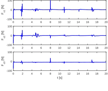
also satisfactory. Fig. 6 shows control input Fo which is smooth and bounded. In Fig. 7, the motion of the object is plotted in Cartesian space, which illustrates that the tracking performance is satisfactory and the proposed control (29) has the ability to guarantee the output constraint. By analysing the above simulation results, it is known that the proposed control (29) can make the system output remain in the corresponding predefined constraint region.

Case two: In the second case, the wall is0.8m away from the coordinate originOalongZ axis, therefore the coordinate of the wall is expressed as (X = 0, Y = 0, Z = 0.8). For convenience, hereafter the location of the wall will be abbreviated as Z = 0.8m. The simulation procedure is that the object carried by two robots moves along the desired trajectory xc from initial position to the wall (Z = 0.8m) in a free space and then after touching the wall, the object slides along the wall, finally leaves the wall and continues moving along the desired trajectory xc in a free space. It should be emphasized that when the object toughs the wall and then slides along it, the interaction between the robot and the wall develops. Consequently, the simulation aim is to verify the effectiveness of the proposed control (29) with interaction between the robot and the wall. The frontier of the output constraint iskc1= 1 + 0.1 sin(t),kc2= 1.11 + 0.1 sin(t)and kc3 = 1.31−0.1 cos(t). The rest of the parameters are the

same as those of case one.

The simulation results of case two are presented in Figs. 8-11. It is known from Fig. 8 that the object moves along the the desired trajectory xc, and slides along the wall when maintaining in contact with the wall. When the object slides along the wall, the target impedance is achieved, and the interaction force between the robot and the wall regulars the control input in order to improve this interaction. Fig. 8 also shows that corresponding time-varying constraint isn’t violated. In Fig. 9, it is obvious that tracking errorz1converges

to a small value near zero. Fig. 10 shows the control input. It is noted that there are a few oscillations while the object comes in contact with the wall. This is due to the change in the unknown environment, but the control force tends immediately to be smooth by using the proposed control (29). In Fig. 11, it is seen that the object moves along the desired trajectory

xc from initial position to the wall, and after encountering the wall, the object slides along the wall, then continues moving to initial position along the desired trajectory xc. Therefore, by analysing the simulation results, we know that the proposed control (29) with impedance learning and time-varying con-straint can improve the environment-robot interaction better,

and make the system output remain in the corresponding time-varying constraint region.

B. Control Design with Full-State Constraint

Case three: In the three case, the simulation procedure

is the same as that of case one. The simulation aim is to verify the effectiveness of the proposed control (53) without interaction between the robot and its environment. Controller parameters are k11 = k12 = k13 = 20. The frontier of the

state constraint is kd1 =kd2 =kd3 = 1.3 + 0.2 cos(t). The

rest of the parameters are the same as those of case one. The simulation results of case three are presented in Figs. 12-16. It can be known from Fig. 12 that two robots can carry the object along the desired trajectory xc in desired

accuracy. And x1i is constrained by time-varying constraint

bound kci, i = 1,2,3. Fig. 13 shows tracking errors which converge to a small value near zero. Fig. 14 shows velocity variable x2i which is constrained by time-varying constraint kdi, i = 1,2,3. Fig. 15 shows control input Fo which is smooth. Fig. 16 shows that actual movement trajectory x1

converges to the desired trajectoryxcgenerated by impedance learning in a short period. Therefore, by analysing the simula-tion results, we know that the proposed control (53) with the full-state time-varying constraint can make the system states remain the corresponding predefined constraint region.

Case four: In the four case, the simulation procedure is

the same as that of case two. The simulation aim is to verify the effectiveness of the proposed control (53) with interaction between the robot and its environment. Controller parameters are k11 = k12 = k13 = 20. The frontier of the state

constraint is kd1 =kd2 =kd3 = 1.3 + 0.2 cos(t)and kc1 =

1 + 0.1 sin(t), kc2= 1.31 + 0.1 sin(t), kc3= 1.31−0.1 cos(t).

The rest of the parameters are the same as those of case one. The simulation results of case four are presented in Figs. 17-21. In Fig. 17, the object tracks the desired trajectoryxc,

slides along the wall when maintaining contact in with the wall, and continues tracking the desired trajectory xc after leaving the wall. In Fig. 18, it is obvious that tracking error

z1converges to a small value near zero. Figs. 17 and 19 show

that full-state constraint cannot be violated, which states that the proposed control (53) has the ability to guarantee the full-state constraint. Fig. 20 shows the control input. It is noted that there are a few oscillations while the object comes in contact with the wall. This is due to the change in the unknown environment, but the control force tends immediately to be smooth by using the proposed control (53). Fig. 21 gives the motion of the object in Cartesian space. Therefore, we know that the proposed control (53) with impedance learning and the full-state time-varying constraint can improve the environment-robot interaction better, and make the system states remain in the corresponding time-varying constraint region.

V. CONCLUSION

(10)

0 2 4 6 8 10 12 14 16 18 20 0.5

1 1.5

x11

[m]

x11

xc1

kc1

0 2 4 6 8 10 12 14 16 18 20

0.5 1 1.5

x12

[m]

x

12

xc2

kc2

0 2 4 6 8 10 12 14 16 18 20

t [s] 0.5

1 1.5

x13

[m]

x13

xc3

[image:10.612.52.528.62.719.2]

kc3

Fig. 4. Case one: Tracking performance

0 2 4 6 8 10 12 14 16 18 20

-0.02 0 0.02

z11

[m]

0 2 4 6 8 10 12 14 16 18 20

-0.01 0 0.01

z12

[m]

0 2 4 6 8 10 12 14 16 18 20

t [s] 0

0.005 0.01

z13

[m]

Fig. 5. Case one: Tracking error

0 2 4 6 8 10 12 14 16 18 20

-100 0 100

Fo1

[N]

0 2 4 6 8 10 12 14 16 18 20

-100 0 100

Fo2

[N]

0 2 4 6 8 10 12 14 16 18 20

t [s] -100

-50 0

Fo3

[N]

Fig. 6. Case one: Control input

0.5 0.6

1 0.7

1 0.8

x13

[m]

0.8 0.9

0.8

x₁₂[m] 1

x₁₁[m] 0.6

1.1

0.6 0.4 0.4

0.2

Actual movement trajectory x1

Desired trajectory xd

Initial position

Fig. 7. Case one: The object’s actual movement trajectory in Cartesian space

0 2 4 6 8 10 12 14 16 18 20

0.5 1 1.5

x11

[m]

x11

xc1

kc1

0 2 4 6 8 10 12 14 16 18 20

0.5 1 1.5

x12

[m] x12

xc2

kc2

0 2 4 6 8 10 12 14 16 18 20

t [s] 0.5

1 1.5

x13

[m]

x13

xc3

kc3

[image:10.612.345.521.66.201.2]

Wall

Fig. 8. Case two: Tracking performance

0 2 4 6 8 10 12 14 16 18 20

-0.05 0 0.05

z11

[m]

0 2 4 6 8 10 12 14 16 18 20

-0.05 0 0.05

z12

[m]

0 2 4 6 8 10 12 14 16 18 20

t [s] -0.05

0 0.05

z13

[m]

Fig. 9. Case two: Tracking error

0 2 4 6 8 10 12 14 16 18 20

-100 0 100

Fo1

[N]

0 2 4 6 8 10 12 14 16 18 20

-100 0 100

Fo2

[N]

0 2 4 6 8 10 12 14 16 18 20

t [s] -100

-50 0

Fo3

[N]

Fig. 10. Case two: Control input

0.5 0.6

1 0.7

1 0.8

x13

[m]

0.8 0.9

0.8

x₁₂[m] 1

x11[m] 0.6

1.1

0.6 0.4 0.4

0.2

Actual movement trajectory x1

Initial position Wall

[image:10.612.83.257.73.206.2]

(11)

0 2 4 6 8 10 12 14 16 18 20 0.5

1 1.5

x11

[m]

x11

xc1

kc1

0 2 4 6 8 10 12 14 16 18 20

0.5 1 1.5

x12

[m]

x

12

xc2

kc2

0 2 4 6 8 10 12 14 16 18 20

t [s] 0.5

1 1.5

x13

[m]

x13

xc3

[image:11.612.347.523.71.194.2]

kc3

Fig. 12. Case three: Tracking performance

0 2 4 6 8 10 12 14 16 18 20

-0.02 0 0.02

z11

[m]

0 2 4 6 8 10 12 14 16 18 20

-0.02 0 0.02

z12

[m]

0 2 4 6 8 10 12 14 16 18 20

t [s] 0

0.005 0.01

z13

[image:11.612.82.258.72.204.2]

[m]

Fig. 13. Case three: Tracking error

0 2 4 6 8 10 12 14 16 18 20

-2 0 2

x21

[m/s]

x21

kd1

-kd1

0 2 4 6 8 10 12 14 16 18 20

-2 0 2

x22

[m/s]

x22

kd2

-kd2

0 2 4 6 8 10 12 14 16 18 20

t [s] -2

0 2

x23

[m/s]

x23

k

d3

-kd3

Fig. 14. Case three: Constrained velocity variablex2

0 2 4 6 8 10 12 14 16 18 20

-100 0 100

Fo1

[N]

0 2 4 6 8 10 12 14 16 18 20

-100 0 100

Fo2

[N]

0 2 4 6 8 10 12 14 16 18 20

t [s] -100

-50 0

Fo3

[N]

Fig. 15. Case three: Control input

0.5 0.6

1 0.7

1 0.8

x13

[m]

0.8 0.9

0.8

x₁₂[m] 1

x₁₁[m] 0.6

1.1

0.6 0.4 0.4

0.2

Actual movement trajectory x

1

Initial position

Fig. 16. Case three: The object’s actual movement trajectory in Cartesian space

0 2 4 6 8 10 12 14 16 18 20

0.5 1 1.5

x11

[m]

x

11

xc1

kc1

0 2 4 6 8 10 12 14 16 18 20

0.5 1 1.5

x12

[m]

x12

xc2

k

c2

0 2 4 6 8 10 12 14 16 18 20

t [s] 0.5

1 1.5

x13

[m]

x

13

xc3

kc3

Wall

Fig. 17. Case four: Tracking performance

0 2 4 6 8 10 12 14 16 18 20

-0.05 0 0.05

z11

[m]

0 2 4 6 8 10 12 14 16 18 20

-0.05 0 0.05

z12

[m]

0 2 4 6 8 10 12 14 16 18 20

t [s] -0.05

0 0.05

z13

[image:11.612.343.521.250.385.2]

[m]

Fig. 18. Case four: Tracking error

0 2 4 6 8 10 12 14 16 18 20

-2 0 2

x21

[m/s]

x21

kd1

-kd1

0 2 4 6 8 10 12 14 16 18 20

-2 0 2

x22

[m/s]

x22

k

d2

-kd2

0 2 4 6 8 10 12 14 16 18 20

t [s] -2

0 2

x23

[m/s]

x23

kd3

-kd3

[image:11.612.81.257.592.725.2]