Evolutionary dynamics of competing phenotype structured populations in periodically fluctuating environments

https://doi.org/10.1007/s00285-019-01441-5

Mathematical Biology

Evolutionary dynamics of competing phenotype-structured

populations in periodically fluctuating environments

Aleksandra Ardaševa1_{·Robert A. Gatenby}2_{·Alexander R. A. Anderson}2_·

Helen M. Byrne1·Philip K. Maini1·Tommaso Lorenzi3

Received: 8 May 2019 / Revised: 14 August 2019 © The Author(s) 2019

Abstract

Living species, ranging from bacteria to animals, exist in environmental conditions that exhibit spatial and temporal heterogeneity which requires them to adapt. Risk-spreading through spontaneous phenotypic variations is a known concept in ecology, which is used to explain how species may survive when faced with the evolutionary risks associated with temporally varying environments. In order to support a deeper understanding of the adaptive role of spontaneous phenotypic variations in fluctuating environments, we consider a system of non-local partial differential equations mod-elling the evolutionary dynamics of two competing phenotype-structured populations in the presence of periodically oscillating nutrient levels. The two populations undergo heritable, spontaneous phenotypic variations at different rates. The phenotypic state of each individual is represented by a continuous variable, and the phenotypic landscape of the populations evolves in time due to variations in the nutrient level. Exploiting the analytical tractability of our model, we study the long-time behaviour of the solu-tions to obtain a detailed mathematical depiction of the evolutionary dynamics. The results suggest that when nutrient levels undergo small and slow oscillations, it is evolutionarily more convenient to rarely undergo spontaneous phenotypic variations. Conversely, under relatively large and fast periodic oscillations in the nutrient levels, which bring about alternating cycles of starvation and nutrient abundance, higher rates of spontaneous phenotypic variations confer a competitive advantage. We discuss the implications of our results in the context of cancer metabolism.

Keywords Periodically fluctuating environments·Evolutionary dynamics· Spontaneous phenotypic variation·Bet-hedging·Non-local partial differential equations

Mathematics Subject Classification 35Q92·92C50·92D25·35K55

B

tl47@st-andrews.ac.uk

1 Introduction

Organisms of various scales, ranging from bacteria to animals, exist in fluctuating environments. For example, in order to cope with changes in nutrient availability, they are required to adapt. When the fluctuations are regular and the populations have sufficient time to sense the changes and react, a highly plastic phenotype, which allows individuals in the population to acquire different traits based on environmental cues, is an optimal strategy (Xue and Leibler2018). An alternative strategy that is more suitable for dealing with irregular and unpredictable changes in the environ-ment is risk spreading, which is also known as bet-hedging (Cohen1966). Here, the population diversifies its phenotypes such that each sub-population is adapted to a specific environment. This ensures that at least some fraction of the population will survive in the face of sudden environmental changes (Philippi and Seger1989). Phe-notypic heterogeneity, a characteristic feature of a risk spreading strategy, is observed in many systems, including bacterial populations (Kussell and Leibler2005) and solid tumours (Marusyk et al.2012).

Bet-hedging is typically proposed to occur within the context of bacterial pop-ulations, where experimental support for stochastic phenotype switching is avail-able (Kussell and Leibler 2005; Smits et al.2006; Veening et al. 2008; Beaumont et al.2009; Acar et al.2008). The classic example of bet-hedging is bacterial persis-tence. During antibiotic treatment a small fraction of slowly growing bacteria, that are resistant to the antibiotic, is able to survive. After the treatment is over, the original population is restored, resulting in resistance to the antibiotic (Balaban et al.2004). Schreiber et al. (2016) showed that fluctuations in nutrient levels alter the metabolism of bacteria and promote phenotypic heterogeneity. Risk spreading strategies have been observed in other organisms, such as fungi and slime moulds (Kussell and Leibler 2005). It is also hypothesized to be present in cancer where irregular vasculature can cause significant fluctuations within the tumour microenvironment (Gillies et al. 2018). Experimental and theoretical work suggest that intermittent lack of oxygen, i.e. cycling hypoxia, leads to clonal diversity, promotes metastasis and selects for more aggressive phenotypes (Cairns et al.2001; Robertson-Tessi et al.2015; Chen et al. 2018; Nichol et al.2016).

was shown to be most successful in an environment that fluctuates on an intermediate timescale.

Most of the experimental and theoretical models that have been developed to explore the dynamics of phenotypic changes in fluctuating environments consider the state of the environment and the phenotypic state of the individuals to be binary—i.e. the environment switches between two extreme conditions and individuals are allowed to jump between two antithetical phenotypic states that are each adapted to opposing environmental conditions (Acar et al.2008; Müller et al.2013; Wienand et al.2017). However, in many cases of biological and ecological interestNatura non facit saltus, and it might therefore be relevant to consider the occurrence of intermediate environ-mental conditions and the existence of a spectrum of possible phenotypic states.

In light of these considerations, we present here a novel mathematical model for the evolutionary dynamics of two competing phenotype-structured populations in periodi-cally fluctuating environments. The phenotypic state of each individual is represented by a continuous variable, and the phenotypic fitness landscape of the populations evolves in time due to variations in the concentration of a nutrient. In order to assess the evolutionary role that heritable, spontaneous phenotypic variations play in envi-ronmental adaptation, we focus on the case where the two populations undergo such phenotypic variations with different probabilities.

In our model, the phenotype distribution of the individuals within each population is described by a population density function that is governed by a parabolic partial differential equation (PDE), whereby a linear diffusion operator models the occur-rence of spontaneous phenotypic variations, while a non-local reaction term takes into account the effects of asexual reproduction and intrapopulation competition. The two non-local parabolic PDEs for the population density functions are coupled through an additional non-local term modelling the effects of interpopulation competition. In such a mathematical framework, the fact that the two populations undergo phenotypic variations with different probabilities translates into the assumption that the two PDEs have different diffusion coefficients.

novel extension of the methods developed in Lorenzi et al. (2015a) to characterise the qualitative and quantitative properties of the solutions.

Exploiting the analytical tractability of our model, we study the long-time behaviour of the solutions in order to obtain a detailed mathematical depiction of the evolutionary dynamics. Moreover, the asymptotic results are compared to numerical solutions of the model equations. Our analytical and numerical results clarify the role of heritable, spontaneous phenotypic variations as drivers of adaptation in periodically fluctuating environments.

The paper is organised as follows. In Sect.2we introduce the mathematical model. In Sect.3we carry out an analytical study of evolutionary dynamics. In Sect. 4we integrate the analytical results with numerical simulations. In Sect.5we discuss the biological relevance of our theoretical findings in the context of cancer cell metabolism and tumour–microenvironment interactions. Section6concludes the paper and pro-vides a brief overview of possible research perspectives.

2 Model description

We study the evolutionary dynamics of two competing phenotype-structured pop-ulations in a well-mixed system. Individuals within the two poppop-ulations reproduce asexually, die and undergo heritable, spontaneous phenotypic variations. We assume the two populations differ only in the rate at which they undergo phenotypic variations. We label the population undergoing phenotypic variations at a higher rate by the letter

H, while the other population is labelled by the letterL.

We represent the phenotypic state of each individual by a continuous variablex∈R, and we describe the phenotype distributions of the two populations at timet ∈ [0,∞)

by means of the population density functions nH(x,t) ≥ 0 andnL(x,t) ≥ 0.

We define the size of populationH, the size of populationLand the total number of individuals inside the system at timet, respectively, as

ρH(t)=

RnH(x,t)dx, ρL(t)=

RnL(x,t)dx, ρ(t)=ρH(t)+ρL(t). (1) Moreover, we define, respectively, the mean phenotypic state and the related variance of each populationi ∈ {H,L}at timetas

μi(t)=

1

ρi(t)

Rx ni(x,t)dx, σ

2

i (t)=

1

ρi(t)

Rx

2

ni(x,t)dx−μ2i(t). (2)

In the mathematical framework of our model, the functionσ_i2(t)provides a measure of the level of phenotypic heterogeneity in theit hpopulation. Finally, we introduce a functionS(t)≥0 to model the concentration of a nutrient that is equally available to the two populations at timet, which we assume is given.

⎧ ⎪ ⎨ ⎪ ⎩

∂nH

∂t =βH

∂2_n

H

∂x2 + R

x,S(t), ρ(t)nH,

∂nL

∂t =βL

∂2_n

L

∂x2 + R

x,S(t), ρ(t)nL,

for(x,t)∈R×(0,∞). (3)

In the system of PDEs (3), the diffusion terms model the effects of spontaneous phenotypic variations, which occur at ratesβH >0 andβL >0, with

βH > βL. (4)

The functional Rx,S(t), ρ(t)models the fitness of individuals in the phenotypic statexat timetunder the environmental conditions given by the nutrient concentration

S(t)and the total number of individualsρ(t)—i.e. the functionalRx,S(t), ρ(t)can be seen as the phenotypic fitness landscape of the two populations at timet. Throughout the paper, we define this fitness functional as

Rx,S, ρ= p(x,S) − dρ. (5)

Definition (5) translates into mathematical terms the following biological ideas: (i) all else being equal, individuals die due to interpopulation and intrapopulation compe-tition at ratedρ(t), with the parameterd >0 being related to the carrying capacity of the system in which the two populations are contained; (ii) individuals in the phe-notypic statexproliferate and die under natural selection at rate p(x,S(t))(i.e. the functionp(x,S)is a net proliferation rate). We focus on a scenario corresponding to the biological assumptions given hereafter.

Assumption 1 Phenotypic variants with x →0have a competitive advantage over the other phenotypic variants when the nutrient concentration is high (i.e. if S(t)1).

Assumption 2 Phenotypic variants with x→1are favoured over the other phenotypic variants when the nutrient concentration is low (i.e. if S(t)1).

Under Assumptions1and2, we define the net proliferation rate as

px,S(t)=γ S(t)

1+S(t) 1−x

2 _{+ ζ}

1− S(t)

1+S(t) 1−(1−x)

2_{, (6)}

with 0< ζ ≤γ. The parametersγ andζmodel, respectively, the maximum prolifer-ation rate of the phenotypic variants best adapted to nutrient-rich and nutrient-scarce environments.

Definition (6) ensures analytical tractability of the model and leads to a fitness functional that is close to the approximate fitness landscapes which can be inferred from experimental data through regression techniques—see, for instance, equation (1) in Otwinowski and Plotkin (2014). In fact, after a little algebra, definition (6) can be rewritten as

0 5 10 S

0 1

x

p(S, x)

<40 91 A

0 10

S 0

1 g(S)

ζ=γ ζ= 0.7γ ζ= 0.2γ

0 10

S 0

1 (S)

0 10

S 0

100 h(S) B

ϕ

Fig. 1 aPlot of the net proliferation ratep(S,x)defined by (6) [or equivalently by (7)] withγ=100 and ζ =50.bThe rescaled maximum fitnessg(S)and the fittest phenotypic stateϕ(S)defined by (8), along with the selection gradienth(S)defined by (9), are plotted against the nutrient concentrationS, forγ=100 and different values of the parameterζ. In this paper we consider the caseζ=γ

with

g(S)= 1

1+S

S+ζ

γ ζ ζ +γS

, ϕ(S)= ζ

ζ +γS (8)

and

h(S)=ζ +(γ−ζ ) S

1+S. (9)

Under the environmental conditions defined by the nutrient concentrationS, the func-tion 0≤ϕ(S)≤1 represents the fittest phenotypic state,γg(S) >0 is the maximum fitness, andh(S)can be seen as a nonlinear selection gradient that quantifies the inten-sity of natural selection. Throughout the paper we will refer tog(S)as the rescaled maximum fitness.

In accordance with Assumptions1and2, Eq. (7) shows that definition (6) is such that the fittest phenotypic state ϕ(S)belongs to the interval[0,1]for any nutrient concentrationS≥0, i.e.ϕ:R_≥0→ [0,1]. In particular, under starvation conditions

(i.e. if S = 0) the fittest phenotypic state is ϕ(0) = 1, while increasing nutrient concentrations correspond to values of the fittest phenotypic state closer to 0, i.e.

ϕ(S) <0 for all S ≥ 0 andϕ(S) → 0 asS → ∞. Furthermore, the fact that the

functionp(x,S)is negative for values ofxsufficiently far from the fittest phenotypic stateϕ(S)captures the idea that less fit variants are driven to extinction by natural selection. These observations are illustrated by the plots in Fig.1.

Henceforth for simplicity we assume

Under assumption (10), definitions (8) and (9) become, respectively,

g(S)= 1

1+S

S+ 1

1+S

, ϕ(S)= 1

1+S and h(S)≡γ. (11)

Moreover, since we assume the functionS(t)to be given, we use the notation

g(t)≡g(S(t)) and ϕ(t)≡ϕ(S(t)).

3 Analysis of evolutionary dynamics

To obtain an analytical description of the evolutionary dynamics, we focus on a bio-logical scenario whereby the initial phenotype distributions of the two populations are Gaussians, that is, we study the behaviour of the solution to the system of non-local parabolic equations (3) subject to the initial condition given by the pairnH(x,0)and

nL(x,0)with

ni(x,0)=ρi0

v0

i

2π exp

−v0i

2 x−μ

0

i 2

for i∈ {H,L}, (12)

whereρ_i0∈R_>0,v_i0∈R>0andμ0_i ∈R.

Remark 1 The choice of initial condition (12) is consistent with much of the

previ-ous work on the mathematical analysis of the evolutionary dynamics of continuprevi-ous traits, which relies on the prima facie assumption that population densities are Gaus-sians (Rice2004).

Before turning to the case of periodically fluctuating environments in Sect. 3.2, we consider the case of constant environments in Sect.3.1. The proofs of the results presented in Sect.3.1and Sect.3.2rely on the results established by Proposition1.

Proposition 1 Under assumptions(5),(7)and(11), the system of non-local PDEs(3)

subject to the initial condition(12)admits the exact solution

ni(x,t)=ρi(t)

vi(t)

2π exp

−vi(t)

2 (x−μi(t))

2

for i ∈ {H,L}, (13)

with the population size,ρi(t), the mean phenotypic state,μi(t), and the inverse of

the related variance,vi(t)=1/σ_i2(t), being solutions of the Cauchy problem ⎧

⎪ ⎪ ⎪ ⎪ ⎪ ⎪ ⎨ ⎪ ⎪ ⎪ ⎪ ⎪ ⎪ ⎩

vi(t)=2 γ−βiv2i(t)

, μi(t)=

2γ

vi(t)(ϕ(

t)−μi(t)),

ρi(t)=(Fi(t)−dρ(t)) ρi(t),

vi(0)=v_i0, μi(0)=μ0_i, ρi(0)=ρ_i0,

ρ(t)=ρH(t)+ρL(t),

where

Fi(t)≡Fi(t, vi(t), μi(t))=γg(t)− γ

vi(t)−γ (μ

i(t)−ϕ(t))2. (15)

Proof Substituting definitions (5), (7) and (11) into the non-local PDE (3) forni(x,t)

yields

∂ni

∂t =βi

∂2_n

i

∂x2 +

γg(t)−γ (x−ϕ(t))2−dρ(t)

ni, ni ≡ni(x,t). (16)

Building upon the results presented in Almeida et al. (2019), Chisholm et al. (2016) and Lorenzi et al. (2015a), we make the ansatz (13) and substituting this ansatz into Eq. (16) we find

ρi

ρi +

vi

2vi =

vi

2 (x−μi)

2_−μ

ivi(x−μi)+βi

v2

i (x−μi)2−vi

+γg(t)−γ (x−ϕ(t))2−dρ. (17)

Equating the coefficients of the zero-order, first-order and second-order terms in x

in (17) produces a system of differential equations. Namely, the second-order terms inxyield the following differential equation forvi alone

vi+2βivi2=2γ. (18)

Moreover, equating the coefficients of the first-order terms inx, and eliminatingv_i from the resulting equation, yields

μi =

2γ (ϕ−μi)

vi .

(19)

Lastly, choosingx=μi in Eq. (17) gives

ρi

ρi +

vi

2vi = −β

ivi+γg−γ (μi−ϕ)2−dρ (20)

and eliminatingv_i from Eq. (20) we find

ρi =(Fi−dρ) ρi, (21)

with the functionFi(t)being defined according to (15). Under the initial condition (12),

we have

vi(0)=vi0, μi(0)=μ0i and ρi(0)=ρi0.

3.1 Evolutionary dynamics in constant environments

Focussing on the case of constant environments, we let the nutrient concentration be constant and thus we make the assumption

S(t)≡S≥0, (22)

which implies that

g(t)≡g and ϕ(t)≡ϕ. (23)

In this case, our main results are summarised by Theorem3.

Theorem 3 Under assumptions(4),(5),(7),(11)and the additional assumption(22), the solution of the system of PDEs(3)subject to the initial condition(12)is of the Gaussian form(13)and satisfies the following:

(i) if

βL ≥√γg (24)

then

lim

t→∞ρH(t)=0 and tlim→∞ρL(t)=0; (25)

(ii) if

βL <√γg (26)

then

lim

t→∞ρH(t)=0, tlim→∞ρL(t)=

√_γ

d

√

γg−βL

(27)

and

lim

t_→∞μL(t)=ϕ, tlim_→∞σ

2

L(t)=

βL

γ . (28)

Proof Under the additional assumption (22), Proposition1ensures that the population

density functionni(x,t)is of the Gaussian form (13) with the population size,ρi(t), the

mean phenotypic state,μi(t), and the inverse of the related variance,vi(t)=1/σ_i2(t),

being governed by the Cauchy problem (14) withg(t)≡gandϕ(t)≡ϕ.

In this framework, we divide the proof of Theorem3into four steps. We study the asymptotic behaviour ofvi(t),μi(t)andFi(t)fort → ∞(Step 1). We show that

ρi(t)is non-negative and uniformly bounded (Step 2). Finally, we prove claim (25)

(Step 3), and we conclude with the proof of claims (27) and (28) (Step 4).

Step 1: asymptotic behaviour of vi(t),μi(t)and Fi(t)for t → ∞. Solving the

separable first-order differential equation (14)1forvi(t)and imposing the initial

con-dition (14)4gives

vi(t)=

_γ

βi

√

γ /βi+v0_i − √

γ /βi−v_i0

exp−4√γ βit √

γ /βi+v_i0+ √

γ /βi−v_i0

exp−4√γβit

which implies that

vi(t)→

_γ

βi

exponentially fast ast→ ∞. (30)

Moreover, solving the differential equation (14)2forμi(t)by the integrating factor

method and imposing the initial condition (14)4yields

μi(t)=μ0i exp

−2γ

t

0

ds

vi(s)

+ϕ

1−exp

−2γ

t

0

ds

vi(s)

, (31)

from which, using the positivity ofvi(t), we find that

μi(t)→ϕ exponentially fast ast → ∞. (32)

Lastly, noting that, under the additional assumption (22), the function Fi(t)defined

by (15) reads as

Fi(t)=γg− γ

vi(t)−γ (μi(

t)−ϕ)2, (33)

the asymptotic results (30) and (32) allow us to conclude that

Fi(t)→γg−

γ βi exponentially fast ast→ ∞. (34)

Step 2: non-negativity and boundedness of ρi(t). Solving the differential

equa-tion (14)3forρiand imposing the initial condition (14)4yields

ρi(t)=ρi0exp

t

0

(Fi(s)−dρ(s))ds

. (35)

This result, along with the positivity ofρ_i0, implies that

ρi(t)≥0 for allt ≥0. (36)

Moreover, substituting (33) into the differential equation (14)3forρi yields

ρi(t)=

γg− γ

vi(t)−γ (μ

i(t)−ϕ)2

ρi(t)−d

ρi(t)+ρj(t)

ρi(t),

with j =Lifi =Handj =Hifi =L. Estimating from above the right-hand side of the latter differential equation by using the non-negativity ofρj(t)[cf. the uniform

lower bound (36)], the positivity ofvi(t)[cf. expression (29)] and the fact thatg<2

[cf. definition (11)], we obtain the differential inequality

which gives the uniform upper bound

ρi(t)≤max

ρ0

i,

2γ

d

for allt ≥0. (37)

Step 3: proof of claim (25). Combining the asymptotic result (34) with the expres-sion (35) forρi we find that

ρi(t)∼Cρi0exp γg−

γ βi

t−d

t

0 ρ(

s)ds

as t → ∞, (38)

for some positive constantC. Since the functionρ(t)is non-negative [cf. the uniform lower bound (36)], the asymptotic relation (38) ensures that

if βi ≥√γg then lim

t→∞ρi(t)=0. (39)

Under assumption (4) and the additional assumption (24), claim (25) follows from the asymptotic result (39).

Step 4: proof of claims(27)and (28). As long asρH(t) > 0, we can compute the

quotient ofρL(t)andρH(t)through (35). In so doing we find

ρL(t)

ρH(t)

= ρ0L

ρ0

H

exp

t

0 (

FL(s)−FH(s))ds

. (40)

Using the limit (34) forFi, we then have

ρL(t)

ρH(t)

∼Cexp _√

γ βH−

βL

t

as t → ∞, (41)

for some positive constantC. Under assumption (4), the asymptotic relation (41) gives

lim

t→∞

ρL(t)

ρH(t)= ∞

and, sinceρL is uniformly bounded from above [cf. the uniform upper bound (37)],

from (41) we conclude that

ρH(t)→0 exponentially fast ast → ∞. (42)

We can rewrite the differential equation (14)3forρLas

ρL(t)= γg−

γ βL+η(t)

−dρL(t)

ρL(t), (43)

where the functionη(t)is defined as

η(t)=γ βL− γ

vL(t)

Using the asymptotic results (30), (32) and (42), we see that

η(t)→0 exponentially fast ast→ ∞. (44)

Solving the differential equation (43) complemented with the initial conditionρL(0)=

ρ0

L yields (Chisholm et al.2016)

ρL(t)=

ρ0

Lexp

t

0

γg−γ βL+η(s)

ds

1+dρ0_L

t

0

exp

s

0 γ

g−γ βL+η(z)

dz

ds

. (45)

The result (44) ensures that in the asymptotic regimet→ ∞we have

exp

t

0 γ

g−γ βL+η(s)

ds

∼C exp γg−γ βL

t

and, under the additional assumption (26), we also have

t

0

exp

s

0

γg−γ βL +η(z)

dz

ds∼C exp

γg−√γ βL

t

γg−√γ βL ,

for some positive constant C. These asymptotic relations, along with the expres-sion (45) forρL, allow us to conclude that

lim

t_→∞ρL(t)=

γg−√γ βL

d . (46)

Claims (27) and (28) follow from the asymptotic results (42) and (46), and the asymp-totic results (32) and (30) withi =L.

The asymptotic results established by Theorem3provide a mathematical formali-sation of the idea that in constant environments:

1. populations undergoing spontaneous phenotypic variation at a rate that is too large compared to the maximum fitness will ultimately go extinct [cf. point (i)]; 2. ceteris paribus, if at least one population undergoes spontaneous phenotypic

vari-ation at a rate sufficiently small compared to the maximum fitness [cf. point (ii)] then:

2(a). the population with the lower rate of phenotypic variation will outcompete the other population;

3.2 Evolutionary dynamics in periodically fluctuating environments

We now focus on the case of environments that undergo fluctuations with periodT >0, and we assume the nutrient concentration to be Lipschitz continuous andT-periodic, i.e. we letS: [0,∞)→R_≥0satisfy the assumptions

S∈Lip([0,∞)) and S(t+T)=S(t) for allt ≥0, (47)

which implies that the functionsg(t)andϕ(t)satisfy the assumptions

g, ϕ∈Lip([0,∞)), g(t+T)=g(T) and ϕ(t+T)=ϕ(T) for allt ≥0. (48) Our main results are summarised by Theorem4, the proof of which relies on the results established by Lemmas1and2.

Lemma 1 Under assumptions(5),(7),(11)and(47), the unique real T -periodic solu-tion of the problem

u_i(t)=2√γ βi (ϕ(t)−ui(t)) , for t∈(0,T),

ui(0)=ui(T),

(49)

is

ui(t)=

2√γβiexp

−2√γβit

exp2√γβiT

−1 T

0

exp 2γβis

ϕ(s)ds

+2γβiexp −2

γβit t

0

exp 2γβis

ϕ(s)ds, (50)

and satisfies the integral identity

1

T

T

0

ui(t)dt=

1

T

T

0

ϕ(t)dt. (51)

Lemma 2 Let

Λi =

βi+

√_γ

T

T

0

(ui(s)−ϕ(s))2ds for i ∈ {H,L}, (52)

and

Qi(t)=γg(t)−

γβi −γ (ui(t)−ϕ(t))2 (53)

with ui(t)given by(50). Under assumptions(5),(7),(11),(47)and the additional

assumption

Λi <

√_γ

T

T

0

the unique real non-negative T -periodic solution of the problem

wi(t)=(Qi(t)−dwi(t)) wi(t), for t∈(0,T),

wi(0)=wi(T),

(54)

is

wi(t)=

d−1exp

t

0

Qi(s)ds

T

0

exp

s

0

Qi(z)dz

ds

exp

T

0

Qi(s)ds

−1 +

t

0

exp

s

0

Qi(z)dz

ds

(55)

and satisfies the integral identity

1

T

T

0

wi(t)dt =

√_γ

d

√_γ

T

T

0

g(t)dt−Λi

. (56)

We refer the interested reader to Lorenzi et al. (2015a) for the proofs of Lemmas1 and2.

Theorem 4 Under assumptions(4),(5),(7),(11)and the additional assumptions(47), the solution of the system of PDEs(3)subject to the initial condition(12)is of the Gaussian form(13)and satisfies the following:

(i) if

min{ΛH, ΛL} ≥

√_γ

T

T

0

g(t)dt (57)

then

lim

t→∞ρH(t)=0 and tlim→∞ρL(t)=0; (58)

(ii) if

min{ΛH, ΛL} <

√_γ

T

T

0

g(t)dt, (59)

and

i =arg min

k∈{H,L}

Λk, j =arg max k∈{H,L}

Λk,

then

ρi(t)→wi(t), ρj(t)→0 as t→ ∞, (60)

and

μi(t)→ui(t), σi2(t)→

βi

γ as t → ∞, (61)

Proof Proposition 1 ensures that the population density functionni(x,t)is of the

Gaussian form (13) with the population size,ρi(t), the mean phenotypic state,μi(t),

and the inverse of the related variance,vi(t)=1/σ_i2(t), being governed by the Cauchy

problem (14). In this framework, we prove Theorem4in 4 steps. In Step 1, we study the asymptotic behaviour ofvi(t),μi(t)andFi(t)fort → ∞. In Step 2, we show that

ρi(t)is non-negative and uniformly bounded. In Step 3, we prove claim (58). Finally,

we prove claims (60) and (61) in Step 4.

Step 1: asymptotic behaviour of vi(t),μi(t)and Fi(t)for t → ∞. Since the

differ-ential equation (14)1does not depend onS(t), the expression (29) ofvi(t)obtained

in the proof of Theorem3still holds and

vi →

_γ

βi

exponentially fast ast → ∞. (62)

Moreover, using the asymptotic result (62) along with the linear differential equa-tion (14)2forμi(t)one can easily show that

μi(t)→ui(t) exponentially fast ast → ∞ (63)

whereui(t)is aT-periodic solution of the differential equation (49). Lemma1ensures

thatui(t)is given by (50). Lastly, forFi(t)defined according to (15), the asymptotic

results (62) and (63) allow us to conclude that

Fi(t)→γg(t)−

γ βi −γ (ui(t)−ϕ(t))2 exponentially fast ast → ∞. (64)

Step 2: non-negativity and boundedness of ρi(t). Proceeding in a similar way as in

the proof of Theorem3(cf. Step 2 in the proof of Theorem3), one can prove that

0≤ρi(t)≤max

ρ0

i,

2γ

d

for allt≥0. (65)

Step 3: proof of claim(58). Solving the differential equation (14)3forρiand imposing

the initial condition (14)4yields

ρi(t)=ρi0exp

t

0

(Fi(s)−dρ(s))ds

, (66)

withFi(t)defined according to (15). Combining the asymptotic result (64) with the

expression (66) forρi(t)gives

ρi(t)∼Cρi0exp

γ

t

0

g(s)ds−γ βit−γ t

0

(ui(s)−ϕ(s))2ds

−d

t

0ρ(

s)ds

for some positive constantC. Hence, using the fact that the functionsg(t),ϕ(t)and

ui(t)areT-periodic and considering m→ ∞, we find

ρi(t)∼Cexp

γm T

0

g(t)dt−mTγ βi −γm T

0

(ui(t)−ϕ(t))2 dt

−d

t

0

ρ(s)ds

ast → ∞, (68)

for some positive constantC. Since the functionρ(t)is non-negative [cf. the uniform lower bound (65)], the asymptotic relation (68) ensures that if

βi +

√_γ

T

T

0

(ui(t)−ϕ(t))2dt ≥

√_γ

T

T

0

g(t)dt

then

lim

t→∞ρi(t)=0. (69)

This proves that if assumption (57) is satisfied then claim (58) is verified.

Step 4: proof of claims(60)and(61). Let

i =arg min

k∈{H,L}

Λk and j =arg max k∈{H,L}

Λk. (70)

As long asρj(t) >0, we can compute the quotient ofρi(t)andρj(t)through (66).

In so doing, using the asymptotic relation (67) forρi(t)andρj(t)and considering

m→ ∞we obtain

ρi(t)

ρj(t) ∼

Cexp

mT√γ Λj −Λi

ast→ ∞, (71)

for some positive constantC, withΛiandΛjdefined according to (52). The asymptotic

relation (71) allows us to conclude that

lim

t→∞

ρi(t)

ρj(t) = ∞.

(72)

Sinceρi is uniformly bounded from above [cf. the uniform upper bound (65)], the

asymptotic result (72) implies that

ρj(t)→0 exponentially fast ast → ∞. (73)

We can rewrite the differential equation (14)3forρi as

ρi(t)=

γg(t)−γ βi −γ (ui(t)−ϕ(t))2+η(t)−dρi(t)

where the functionη(t)is defined as

η(t)=γ βi− γ

vi(t)

+γ (ui(t)−ϕ(t))2−(μi(t)−ϕ(t))2

−dρj(t).

Using the asymptotic results (62), (63) and (73) we see thatη(t)→0 exponentially fast ast → ∞. Hence,ρi(t)→ ˜ρi(t)ast → ∞, withρ˜i(t)being the solution of the

differential equation

˜

ρi = f(ρ˜i,t), (75)

with

f(ρ˜i,t)=

γg(t)−γ βi−γ (ui(t)−ϕ(t))2−dρ˜i

˜

ρi,

subject to an initial condition 0<ρ˜i(0) <∞. We note that: (i) the functionρ˜i(t)is

uniformly bounded as it satisfies the upper and lower bounds

0≤ ˜ρi(t)≤max

˜

ρi(0),

2γ

d

for allt≥0;

(ii) the function f is Lipschitz continuous in the first variable; (iii) the function f is Lipschitz continuous andT-periodic in the second variable, sinceg,ϕ andui areT

-periodic Lipschitz continuous functions oft[cf. assumptions (48) and expression (50)]. Therefore, the conditions of Massera’s Convergence Theorem (Massera et al.1950; Smith1986) are satisfied and this allows us to conclude that

˜

ρi(t)−→wi(t) ast → ∞, (76)

withwi(t)being a non-negativeT-periodic solution of the differential equation (54).

Under the additional assumption (59), that is,

Λi <

√_γ

T

T

0

g(t)dt,

Lemma2ensures thatwi(t)is given by (55). Claims (60) and (61) follow from the

asymptotic results (73) and (76) along with the asymptotic result (63) and (62) with

i =arg min

k∈{H,L}

Λk.

In summary, Theorem4gives an explicit characterisation of the long-term limit of

vi(t),μi(t)andρi(t) for the surviving populationi and shows that the surviving

population is the one characterised by the larger positive value of the quantity

1

T

T

0

F_i∞(t)dt= γ T

T

0

where

F_i∞(t)= lim

t_→∞Fi(t)=γg(t)−

γβi −γ (ui(t)−ϕ(t))2.

Remark 2 Since the functionsui(t)andwi(t)areT-periodic and satisfy the integral

identities (51) and (56), respectively, the results established by Theorem4show that the long-term limits of the size and the mean phenotypic state of the surviving population are periodic functions of time with periodT and mean values given by (51) and (56), respectively.

Remark 3 Using the differential equation (49) forui(t)one can easily obtain

d

dt (ui−ϕ)

2₌

4γγ βi

1 2

1 √

γ βi (ϕ−

ui) ϕ −(ui −ϕ)2

.

Integrating both sides of the above equation with respect tot between 0 andT, and using the fact thatui(T)−ϕ(T)=ui(0)−ϕ(0), yields

1

T

T

0

(ui(t)−ϕ(t))2 dt=

1 2√γ βi

1

T

T

0

(ϕ(t)−ui(t)) ϕ(t)dt. (77)

Therefore, definition (52) can be rewritten as

Λi =

βi+

1 2√βi

1

T

T

0

(ϕ(t)−ui(t)) ϕ(t)dt. (78)

IfS≡ ¯Stheng(t)≡gandϕ(t)≡ϕ(i.e.ϕ ≡0). In this case, √_γ

T

T

0

g(t)dt=g

and (78) allows one to see thatΛi =

√

βi. Hence, if S is constant then the results

of Theorem 4 reduce to the results of Theorem3. Moreover, the first term in the expression (78) forΛi is clearly a monotonically increasing function ofβi, whereas

the factor in front of the integral in the second term is a monotonically decreasing function ofβi. Hence, if the mean value of theT-periodic function(ϕ(t)−ui(t)) ϕ(t)

is sufficiently small thenΛH > ΛL, while if such a mean value is sufficiently large

thenΛH < ΛL. We expect the latter scenario to occur when the variability and the

rate of change ofS(t)are sufficiently high so as to cause substantial and sufficiently fast variations in the value ofϕ(t).

The asymptotic results established by Theorem4formalise mathematically the idea that in periodically fluctuating environments:

2. ceteris paribus, if at least one population undergoes spontaneous phenotypic vari-ations at a rate sufficiently small compared to the mean value of the maximum fitness, then the following behaviours are possible:

2(a). when environmental conditions are relatively stable, the population with the lower rate of phenotypic variations will outcompete the other population [cf. point (ii) and Remark3];

2(b). when environmental conditions undergo drastic changes, either both popula-tions go extinct [cf. point (i) and Remark3] or the population with the higher rate of phenotypic variations will outcompete the other population [cf. point (ii) and Remark3];

2(c). the phenotype distribution of the surviving population will be unimodal, and both the population size and the mean phenotype will become periodic [cf. point (ii) and Remark2];

2(d). ultimately, the population size and the mean phenotype will both oscillate with the same period as the fluctuating environment, and the mean value (with respect to time) of the mean phenotype will be the same as the mean value of the fittest phenotypic state with the related variance being directly proportional to the rate of phenotypic variations [cf. point (ii) and Remark2].

These biological implications are reinforced by the numerical solutions presented in the next section.

4 Numerical simulations

In this section, we construct numerical solutions to the system of non-local parabolic PDEs (3) subject to the initial condition (12). In Sect.4.1, we describe the numerical methods employed and the set-up of numerical simulations. In Sect.4.2, we present a sample of numerical solutions that confirm the results of our analysis of evolutionary dynamics, both in the case whereS(t)is constant and whenS(t)oscillates periodically.

4.1 Numerical methods and set-up of numerical simulations

We select a uniform discretisation consisting of 2000 points on the interval[−5,5]as the computational domain of the independent variablexand impose no flux boundary conditions. Moreover, we assumet ∈ [0,tf], withtf > 0 being the final time of

simulations, and we discretise the interval[0,tf]with the uniform stepΔt =0.0001.

The method for constructing numerical solutions to the system of non-local parabolic PDEs (3) is based on an explicit finite difference scheme in which a three-point stencil is used to approximate the diffusion terms and an explicit finite difference scheme is used for the reaction term (LeVeque2007). On the other hand, we use theMatlab

built-in solverode45to solve numerically the Cauchy problem (14) forvi(t),μi(t)

andρi(t).

Table 1 Parameter values used to carry out numerical simulations

Parameter Description Value/value range

γ Maximum proliferation rate 100

d Death rate due to competition 0.01

βL Rate of phenotypic variation of populationL 0.01

βH Rate of phenotypic variation of populationH [0.01, 0.1]

small, in general, and much smaller than maximum proliferation rates, in particular, we assumeβi γ fori ∈ {H,L}. Furthermore, given the values ofγ andβi, we

fix the value ofdto be such that the long-term limit (27) of the size of the population

L is approximatively 104, which is consistent with biological data from the existing literature regarding in vitro cell populations (Voorde et al.2019).

We remark that the value of the parameterβL and the range of values of the

param-eterβH reported in Table1are such that neither condition (24) nor condition (57) are

met in all cases on which we report here. This ensures that the two populations do not simultaneously go extinct.

We consider both populations to have the same initial phenotypic distribution (12) withv0_i =20,μ_i0=0 andρ_i0≈800 fori ∈ {H,L}.

4.2 Main results

We consider the following definition of the nutrient concentration

S(t)=M+Asin

2πt T

. (79)

In definition (79), the parameterM >0 represents the mean nutrient concentration, while the parameter A ≥ 0 models the semi-amplitude of the oscillations of the nutrient concentration, which have periodT >0. Clearly, we consider only values of

M andAsuch thatS(t)≥0, i.e. 0≤ A≤ M.

We start by exploring three prototypical scenarios exemplified by different values of the parameter A. In particular, we choose M = 1 and compare the numerical solutions obtained for A = 0 (i.e. constant nutrient concentration), A = 0.5 (i.e. lower nutrient variability) andA=1 (i.e. higher nutrient variability). Figure2displays plots of the nutrient concentration S(t), the rescaled maximum fitnessg(t)and the fittest phenotypic stateϕ(t)corresponding to such choices of the parameter A. These plots show that, as one would expect, higher nutrient variability brings about more pronounced variations in the rescaled maximum fitness and the fittest phenotypic state. Figure3shows a comparison between the exact solutions (13)—withvi(t),μi(t)

andρi(t)obtained by solving numerically the Cauchy problem (14)—and the

A

B

C 0 1 2

Nutrient level S₍t₎

0.6

0.8

1.0

Maximum fitness g₍t₎

0.0

0.5 1.0

Fittest phenotypic state (t)

0 1 2

0.6

0.8

1.0

0.0

0.5

1.0

0 10 20

t

0 1 2

0 10 20

t

0.6

0.8

1.0

0 10 20

t

0.0 0.5 1.0

ϕ

Fig. 2 aPlots of the nutrient concentrationS(t)(left panel) defined according to (79) withM =1 and

A=0, and the corresponding rescaled maximum fitnessg(t)(central panel) and fittest phenotypic state ϕ(t)(right panel) defined according to (11).bSame as rowabut withA=0.5 andT=5.cSame as row abut withA=1 andT=5

computing numerically the integrals of the components of the numerical solution of the system of PDEs (3) (cf. solid lines in the left column of Fig.3) and the population sizes obtained by solving numerically the Cauchy problem (14) (cf. dashed and dotted lines in the left column of Fig.3). Similarly, there is excellent agreement between the population density functions obtained by solving numerically the system of PDEs (3) (cf. solid lines in the right column of Fig.3) and the population density functions (13) withvi(t),μi(t)andρi(t)given by the numerical solutions of the Cauchy problem (14)

(cf. dashed and dotted lines in the right column of Fig.3).

In accord with the results of Theorem3, when the nutrient concentration is constant (i.e. S(t) ≡ M), the population with the lower rate of phenotypic variations (i.e. populationL) outcompetes the other population (vid. Fig.3a). The size of the surviving populationρL(t)reaches the asymptotic value (27) and the phenotype distribution at

the end of the simulationsnL(x,tf)is Gaussian with mean and variance equal to the

asymptotic values (28).

In agreement with the results established by Theorem4(vid. Remark3), a similar outcome is observed in the presence of a low nutrient variability (vid. Fig.3b). In fact, in this caseΛL < ΛH. On the contrary, the population with the higher rate of

phenotypic variations (i.e. populationH) outcompetes the other population when the nutrient variability is sufficiently high (vid. Fig.3c). This is due to the fact that in this case the conditionΛH < ΛL is met. As expected (cf. Remark2), sinceA>0 both

A

C

0.0 0.5

×104

Population size

ρL

ρL

ρH

ρH 0 2

×104

Phenotype distribution

0.0 0.5

×104

t1

t2

0 2

×104

t1 t2

0 20 40

t

0.0 0.5 1.0 ×10

4

t1 t2

0 1

x

0 2

×104

t1 t2 B

Fig. 3 Left column. Plots of the population sizesρH(t)(red line) andρL(t) (blue line) obtained by

computing numerically the integrals of the components of the numerical solution of the system of PDEs (3) subject to the initial condition (12). The dotted and dashed lines highlight, respectively,ρH(t)andρL(t)

obtained by solving numerically the Cauchy problem (14). The nutrient concentration S(t)is defined according to (79) withM = 1 andA =0 (rowa),M =1, A= 0.5 andT =5 (rowb), orM =1,

A=1 andT=5 (rowc)—cf. the plots displayed in Fig.2. The values of the model parameters are those reported in Table1withβH =0.025. Right column. Plots of the corresponding phenotype distribution

of the surviving population obtained by solving numerically the system of PDEs (3) subject to the initial condition (12). In particular, the plot ofnL(x,tf)is shown in rowa, while the plots in rowsbandcare,

respectively, those ofnL(x,t)andnH(x,t)att =t1andt=t2, witht1andt2being highlighted in the corresponding plots in the left column. The dotted and dashed lines correspond to the exact phenotype distributions (13) withvi(t),μi(t)andρi(t)given by the numerical solutions of the Cauchy problem (14)

(color figure online)

of the surviving population remains Gaussian with variance given by (61). This implies that if population H outcompetes population L then the variance of the phenotype distribution (i.e. the level of phenotypic heterogeneity) will be ultimately larger than in the case where populationLis selected.

Taken together, these results demonstrate that when the nutrient concentration is constant, or in the presence of a low level of nutrient variability, it is evolutionarily more desirable to rarely undergo spontaneous phenotypic variations, since environmental conditions are stable. Conversely, when nutrient variability is high (i.e. alternating cycles of starvation and nutrient abundance occur), higher rates of spontaneous phe-notypic variations constitute a competitive advantage, as they allow for a quicker adaptation to changeable environmental conditions, and higher level of phenotypic heterogeneity emerge.

advan-0.01 0.1 βH

A= 0.5

t

S(t)

t

S(t)

t

S(t)

0.01 0.1

βH 1 20

T

A= 0.5,M= 1.0

0.01 0.1

βH 1 20

T

A= 10.0,M= 60.0

0.01 0.1

βH

A= 1.0

0.01 0.1

βH

A= 10.0

0.01 0.1

βH

A= 25.0

0.01 0.1

βH

A= 50.0

1 20

T

A B

CIntermediate mean, large amplitude

0.2

Low mean, small amplitude High mean, small amplitude

Fig. 4 aQualitative dynamics of the nutrient concentrationS(t)defined according to (79) withM=60 andA=10, and corresponding plot of sgn(ΛH−ΛL)as a function ofβH ∈(βL,0.1], withβL=0.01,

andT ∈ [1,20]. The quantitiesΛH andΛLare computed using (52) and the values of the other model

parameters reported in Table1. The blue points in theβH−Tplane correspond to sgn(ΛH−ΛL)=1

(i.e.ΛL< ΛH), whereas the red points correspond to sgn(ΛH−ΛL)= −1 (i.e.ΛH < ΛL).bSame

as panelabut withM=1 andA=0.5.cSame as panelbbut withM=AandA∈ {0.5,1,10,25,50} (color figure online)

tage. In more detail, as shown by the asymptotic results established by Theorem4, provided that condition (57) is not satisfied (i.e. at least one population survives), the outcome of competition between population Hand populationL in periodically fluctuating environments can be predicted by computing the value of the quantities

ΛH andΛL given by (52). In particular, the population characterised by the lower

value of this quantity will ultimately be selected. Therefore, we computedΛH and

ΛL for different values of the period of the nutrient oscillationsT and different

val-ues of the rate of spontaneous phenotypic variationsβH. We used the values of the

other evolutionary parameters reported in Table1and considered possible values of the environmental parametersMandAcorresponding to three different scenarios: an environment whereby the nutrient is abundant and undergoes small-amplitude peri-odic oscillations, i.e.M is relatively large andAis relatively small (vid. Fig.4a); an environment whereby the nutrient is scarce and undergoes small-amplitude periodic oscillations, i.e.M andAare both relatively small (vid. Fig.4b); and an environment whereby periodic oscillations can induce a sufficiently high variability of nutrient concentration, i.e.M =Aand different values of Aare allowed (vid. Fig.4c).

The results obtained are summarised by the plots in Fig.4. As we would expect (cf. Remark3), if the nutrient concentration undergoes low-amplitude periodic oscillations thenΛL < ΛH for all values ofT andβH considered (vid. Fig.4a, b). On the other

hand, when periodic oscillations can bring about sufficiently high levels of nutrient variability, there is a region of theβH −T plane whereΛH < ΛL (vid. Fig.4c).

When the value of Ais either low or high, this region is small and concentrated in the bottom left corner of the plane. For intermediate values of Athe region where

ΛH < ΛLis wider and such that the smaller the valueT(i.e. the higher the frequency

0 20 40 0

0 1

x

nH(t, x)

0 4×104

0 20 40 1

x

nL(t, x)

0 4×104

0 20 40

t 0 5000 10000 ρi ( t )

0 20 40 0 50 100 S ( t )

A= 0.1,M= 0.1

0.0 0.2

0 20 40 0

1

x

nH(t, x)

0 4×104

0 20 40 0

1

x

nL(t, x)

0 4×104

0 20 40

t 0 5000 10000 ρi ( t ) _ρ

L(t)

ρH(t) 0 20 40 0 50 100 S ( t )

A= 20,M= 70

0 20 40 0

1

x

nH(t, x)

0 3×104

0 20 40 0

1

x

nL(t, x)

0 3×104

0 20 40

t 0 5000 10000 ρi ( t )

0 20 40 0 50 100 S ( t )

A= 50,M= 50

0 20 40 0

1

x

nH(t, x)

0 3×104

0 20 40 0

1

x

nL(t, x)

0 3×104

0 20 40

t 0 5000 10000 ρi ( t )

0 20 40 0 50 100 S ( t )

A= 10,M= 10

A B C D

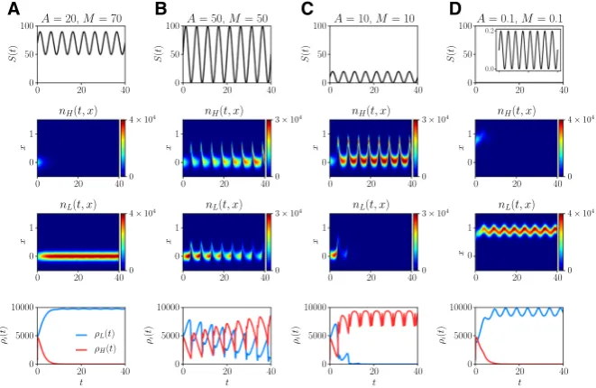
Fig. 5 aPlots of the nutrient concentrationS(t)(first row), the phenotype distributionsnH(x,t)(second

row) andnL(x,t)(third row), and the population sizesρH(t)(fourth row, red line) andρL(t)(fourth row,

blue line) obtained by solving numerically the system of PDEs (3), whereS(t)is defined according to (79) withT =5,A =20 andM =70. The values of the model parameters are defined as in Table1with βH =0.025.b–dSame as column a but for A= M=50 (columnb),A= M =10 (columnc), and

A=M=0.1 (column d) (color figure online)

Furthermore, we can investigate how the fluctuations in the nutrient level affect the phenotypic distribution of each population at any given time point by constructing numerical solutions to the system of non-local PDEs (1) subject to initial condition (12) withS(t)defined according to (79). This is demonstrated by the plots in Fig.5, which show sample dynamics of the nutrient concentrationS(t), the phenotype distributions

nH(x,t)andnL(x,t), and the population sizesρH(x,t)andρL(x,t), for different

values of semi-amplitudeAand meanMof the fluctuations.

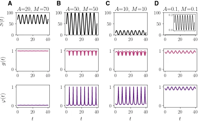
When the nutrient is abundant and experiences fluctuations of relatively low level (vid. Fig.5a) populationLoutcompetes populationH. This is due to the fact that, as shown by Fig.8a in “Appendix”, the fittest phenotypic stateϕ(t)undergoes very small periodic oscillations and its value remains close to 0 (i.e. the value of the phenotypic variablex corresponding to the fittest phenotypic state when nutrient is abundant). Moreover, the rescaled maximum fitnessg(t)undergoes very small periodic oscilla-tions and its value remains close to 1.

When the nutrient level is uniformly low and undergoes relatively small oscilla-tions (vid. Fig.5d) population Lis selected against populationH. This is due to the fact that, as shown by Fig.8d in “Appendix”, both the fittest phenotypic stateϕ(t)

For the cases when the populations experience fluctuations of relatively high level (vid. Fig. 5b, c) population H outcompetes population L. This is due to the fact that, as shown by Fig.8b, c in “Appendix”, the fittest phenotypic stateϕ(t)fluctuates periodically between 1 and a positive value close to 0. Moreover, the rescaled maximum fitnessg(t)undergoes small periodic oscillations and its value remains close to 1.

Note that in all cases the phenotype distribution of the surviving population remains unimodal with maximum at the mean phenotypic state. Ultimately, both the size and the mean phenotypic state of the surviving population oscillate periodically with the same period as the nutrient concentrationS(t). Furthermore, when the populations experi-ence fluctuations of relatively high level (i.e. Figure5b, c), the mean phenotypic state of the surviving population (i.e. populationH) undergoes rapid transitions between 1 and a positive value close to 0. This can be biologically seen as the emergence of a bet-hedging behaviour.

5 Interpretation of the results in the context of cancer metabolism

The generality of the model and the robustness of the results make our conclu-sions applicable to a broad range of asexual populations evolving in fluctuating environments. As an example, in this section we discuss the biological implications of our mathematical results in the context of cancer cell metabolism and tumour– microenvironment interactions.

Cancers begin from single cells that grow to form organ-like masses within mul-ticellular organisms. A fundamental property of cancer cells is a self-defined fitness function such that their proliferation is determined by their heritable phenotypic prop-erties and the local environmental selection forces. That is, individual cancer cells have the capacity to evolve novel phenotypes and to adapt to the often harsh intratumoural environment. In contrast, while normal epithelial cells have the capacity to change their phenotype to some degree, e.g. they can only do so within normal physiological constraints in response to stress. In other words, because the proliferation of normal cells is entirely governed by local tissue constraints, they cannot, unlike cancer cells, evolve adaptations to many non-physiological conditions.

This difference in evolutionary capacity (or reaction norm) can confer a significant adaptive advantage to cancer cells. For example, cancer cells often metabolise glucose using glycolytic (converting glucose to lactic acid) pathways even when the oxygen concentration is sufficient for the aerobic mechanism (converting glucose to H2O

and CO2). Known as the Warburg effect (Warburg1925), this can be understood in a

Darwinian context as a form of niche construction because inefficiency of ATP (energy currency of cells) production is offset by the evolutionary advantage of generating a locally acidic environment. Cancer cells can evolve adaptive strategies to survive and proliferate in such an environment but normal cells cannot.

Fig. 6 Schematic interpretation of the phenotypic fitness landscape of our model in the context of cancer metabolism

imperative to invest resources in vascular maturation that permits blood flow to other regions of the tumour (Gillies et al.2018). Such an unregulated vascular network will be highly unstable with cycles of growth and regression and blood flow dynamics that are inevitably disordered.

A number of studies have demonstrated that this disordered process of angiogenesis produces stochastic variations in blood flow leading to cycles of perfusion, cessation of flow, and then re-perfusion (Kimura et al.1996). This produces corresponding fluc-tuations in local environmental conditions that are dependent on blood flow, including oxygen and glucose, retention of metabolites such as acid, and important signalling molecules such as testosterone or oestrogen. Particularly, regions of normoxia (nor-mal levels of oxygen), chronic hypoxia (low oxygen level) and cycling hypoxia have been distinguished in experimental and clinical studies (Michiels et al.2016). If we assume thatS(t)in our model represents the oxygen level at timet, then the pheno-typic variants best adapted to oxygen-rich environments, and thus displaying a regular metabolism, are those with x → 0, while the phenotypic variants best adapted to oxygen-low environments—i.e. the phenotypic variants that proliferate through the consumption of glucose, which is usually abundant—correspond tox→1. For sim-plicity, we ignore any costs associated with the choice of metabolic preference, so that assumption (10) is satisfied. This is illustrated by the schemes in Fig.6.

Regions of normoxia and chronic hypoxia are analogous to cases a and b in Fig.4 where low levels of environmental variability are observed. Our results support the idea that these regions will be mainly populated by phenotypic variants best adapted to either oxygen-rich or oxygen-low environments. Moreover, since our results indicate that a higher rate of phenotypic variation does not constitute a competitive advantage in the presence of small environmental fluctuations, we expect relatively low levels of phenotypic heterogeneity to be observed in regions of either normoxia or chronic hypoxia.

Fig. 7 Summary of the biological interpretation of our results in the context of cancer metabolism

a survival strategy in response to drastic variation in oxygen levels. These conclusions are summarised in the table provided in Fig.7.

6 Conclusions

We have presented a mathematical model for the evolutionary dynamics of two asexual phenotype-structured populations competing in periodically oscillating environments. The two populations undergo heritable, spontaneous phenotypic variations at differ-ent rates and their fitness landscape is dynamically sculpted by the occurrence of fluctuations in the concentration of a nutrient.

Our analytical results formalise the idea that when nutrient levels experience small and slow periodic oscillations, and thus environmental conditions are relatively stable, it is evolutionarily more efficient to rarely undergo spontaneous phenotypic variations. Conversely, under relatively large and fast periodic oscillations in the nutrient levels, which lead to alternating cycles of starvation and nutrient abundance, higher rates of spontaneous phenotypic variations can confer a competitive advantage, as they may allow for a quicker adaptation to changeable environmental conditions. In the lat-ter case, our results indicate that higher levels of phenotypic helat-terogeneity are to be expected compared to those observed in slowly fluctuating environments. Finally, our results suggest that bet-hedging evolutionary strategies, whereby individuals switch between antithetical phenotypic states, can naturally emerge in the presence of rela-tively large and fast nutrient fluctuations leading to drastic environmental changes.

instance, cells are known to turn to glucose for their energy production when oxygen is in short supply, i.e. they produce energy through anaerobic glycolysis instead of using oxidative phosphorylation that requires aerobic conditions. Since anaerobic glycolysis is far less efficient in terms of produced energy than oxidative phosphorylation (Vander Heiden et al.2009), the proliferation rate of glucose-dependent phenotypic variants might be lower than that of phenotypic variants best adapted to oxygenated environ-ments. Therefore, it would be interesting to extend our analytical results to the case whereζ < γ. It would also be interesting to consider cases where an integral operator is used, in place of a differential operator, to describe the effect of phenotypic vari-ations. In this case, we expect the qualitative behaviour of the results presented here to remain unchanged when the transition between phenotypic states is modelled via Gaussian kernels of sufficiently small variance. From a mathematical point of view, this would require further development of the methods of proof presented here in order to carry out a similar asymptotic analysis of evolutionary dynamics.

Another natural extension of the model is consideration of the feedback from the populations on the nutrient level. In fact, most existing models of evolutionary dynam-ics in a fluctuating environment do not account for this feedback and potentially nonlinear dynamical interactions between individuals and the surrounding environ-ment. However, changes in the population dynamics are known to affect the outcome of interspecies competition in the presence of time variations in the availability of nutrients (Okuyama2015). For instance, in the context of solid tumours, one could consider both negative feedback mechanisms that regulate population growth, such as nutrient consumption, and positive feedback mechanisms that promote the supply of nutrient, such as angiogenesis, i.e. hypoxia-induced formation of blood vessels. Consideration of these mechanisms is expected to affect the advantages gained by each population, and therefore the phenotypic composition of the tumour, in a given environment.