TRIC-track: Tracking by Regression with Incrementally Learned Cascades
Xiaomeng Wang
Michel Valstar
Brais Martinez
Muhammad Haris Khan
Tony Pridmore
Computer Vision Laboratory, University of Nottingham, Nottingham, UK
{psxxw, michel.valstar, brais.martinez, psxmhk, tony.pridmore}@nottingham.ac.uk
Abstract
This paper proposes a novel approach to part-based track-ing by replactrack-ing local matchtrack-ing of an appearance model by direct prediction of the displacement between local image patches and part locations. We propose to use cascaded regression with incremental learning to track generic ob-jects without any prior knowledge of an object’s structure or appearance. We exploit the spatial constraints between parts by implicitly learning the shape and deformation pa-rameters of the object in an online fashion. We integrate a multiple temporal scale motion model to initialise our cas-caded regression search close to the target and to allow it to cope with occlusions. Experimental results show that our tracker ranks first on the CVPR 2013 Benchmark.
1. Introduction
We propose a method for structured object Tracking by Regression with Incrementally learned Cascades (TRIC-track). Visual tracking of generic objects is one of the most active topics in computer vision. It aims to detect the lo-cation of a possibly moving target by extracting local ap-pearance features and matching them between consecutive images to obtain accurate estimates of target location, of-ten helped by similar estimates of the object’s motion. The parameters describing a target object can vary, but often clude position, size, orientation and velocity. Tracking in-formation can subsequently be used to reason about the tar-get’s behaviour or complete other tasks that require knowl-edge of the object’s state. If solved, visual tracking has extensive applications in areas such as visual (robot) navi-gation, surveillance, traffic monitoring, video compression, medical imaging etc.
Despite the large body of computer vision work address-ing this problem, robust visual trackaddress-ing of generic objects is still a challenging problem. The performance of a vi-sual tracking algorithm is affected by many factors, such as non-rigid object deformation, partial or full occlusion of the target, illumination variation, scale variation, viewpoint
(a) (b) (c) (d)
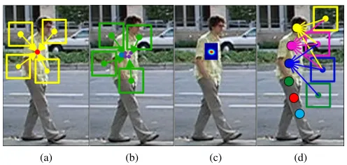
Figure 1: (a) Training a direct displacement regressor with four examples. (b) Testing a regressor. Four test patches sampled around the initial location (blue dot) provide pre-dictions (purple dots). (c) Evidence aggregation map. (d) Location-based initialisation and implicit shape model.
change, motion blur, background clutter, etc. The combi-nation of rigid motion and non-rigid object deformation re-sults in complex appearance changes, making general ob-ject tracking a particularly hard problem.
Current part-based trackers rely upon a response map es-timating the likelihood that any given location in an image represents the target (part). While approaches to the com-putation of this fitness vary from simple template matching to complex machine learning based methods, all assign a single scalar value to a queried location. Tracking then be-comes a problem of determining what area(s) to search in, often guided by some motion model(s), how to construct an appearance model that can capture changes in the object’s image properties, and how to deal with local optima.
While a template likelihood strategy may appear to be the logical solution to the visual tracking problem, its view of the image as a set of independent, possible target loca-tions introduces a number of inherent drawbacks. Firstly, incorrect optima occur when changes in the target’s ap-pearance make it look less like the original template than some background image patch(es), or when there are
[image:1.612.307.555.235.353.2]tiple identical objects (parts) in the scene. Secondly, for the template strategy to work, an entire region of interest needs to be searched. This can be computationally intensive, but methods (e.g. gradient descent) introduced to speed up the search can also converge to local optima. Thirdly, in a tem-plate likelihood strategy local information (be it part of the object foreground or the background) only serves to inform the tracker whether it is the target or not. Once the opti-mal location has been sampled, sampling additional non-optimal local patches does not improve the confidence that this is indeed the target location. It can only make matters worse: increasing the size of the search area only increases the likelihood of falling upon an incorrect optimum. Finally, template likelihood approaches to part-based tracking can-not directly use the appearance of one part to determine the location of another. Although an explicit structure model can be learned to constrain the expected relative positions of parts, such a shape fitting step is effectively bolted-on on top of independent, individual local part trackers.
We propose to replace this local fitness-based approach by direct displacement-based tracking in which we predict the two-dimensional displacement vector between the cen-tre of a sampled image patch and the target (part) location using regressors (see Fig. 1). In doing so, local patches contribute to the solution by directly ‘voting’ for the tar-get (part) location. In addition, while template-based ap-proaches need to model part appearance and shape fitness separately, our direct displacement prediction by regression tracker implicitly learns the shape and possible deforma-tions of an object. It does so by tracking each part using not only the local evidence for that part, but also evidence provided by neighbouring parts.
We adopt cascaded regression [3, 22], specifically the Supervised Descent Method (SDM)[22], which has been successfully applied to the localisation of facial points, for which models were learned offline on very large sets of faces. Cascaded regression makes increasingly smaller steps towards the target location, each regressor in the cas-cade being trained on a smaller region around the ground truth and thus having a smaller expected error. While SDM has been used for what is essentially structured object detec-tion, it has never been used for online model-free tracking. The key difference between detection of a known object and generic object tracking is that appearance and structure models of the former can be learned offline on potentially hundreds of thousands of images, while the models for the latter must be initialised on a single frame.
To learn the appearance changes of our parts over time, we take inspiration from the incremental learning of cas-caded regression proposed by Asthana et al. [1]. That work personalises SDM for facial point localisation, initialising the SDM offline on a large database of faces, and using newly tracked faces to incrementally update it. In our
ap-proach the SDM is initialised on the first frame only, and we use Local Evidence Aggregation [14] of the separate re-gression contributions to provide a confidence level, which is used to decide whether we can use the tracking result to update the SDM.
We report on extensive tests, both internal evaluations to determine the relative value of the various components of our proposed tracker, and comparisons against the current state-of-the-art. Traditional benchmark measures [21] as-sume the target is represented by a bounding box. This is not the case here. Deformable articulated objects often dis-play significant non-rigid deformation during tracking. As a result, parts of the object would either ’stick out’ of the bounding box, or the bounding box would contain large ar-eas of background. The method presented here therefore tracks points, not boxes. This means that the best way to evaluate our system is to compare the predicted and ground truth locations of target parts. However, as this information is not available for the state-of-the-art, we revert to compar-ison based on a retro-fitted bounding box.
In summary, we make the following four contributions:
• We propose direct displacement prediction for the first time in online model-free tracking. By aggregating samples’ predictions, we obtain a robust prediction distribution.
• We implicitly model the shape of a target using local evidence from multiple parts.
• We adapt the framework of SDM [22] to the problem of online tracking of generic objects. We show that it is possible to learn the cascade models on-the-fly without strong supervision.
• We integrate a multiple temporal scale motion model [11], taking the proposed method beyond ’tracking by detection’.
2. Related Work
We divide the related work in two: structured object tracking-by-detection methods, in which the similarity is the aim to track a structured object, and works in which re-gressors were used to perform object alignment. We finally highlight the similarities and differences of our approach with respect to these methods.
Structured tracking-by-detection: Imposing shape
minimising the restrictions imposed by the shape model. Since the number of possible outputs grows exponentially with the number of parts and part hypotheses, it is most common to resort to an efficient shape model, e.g. De-formable Part Models (DPM) [7], where exact inference is possible. These models are often extended to allow for tracking-specific purposes, most commonly using temporal consistency or online/incremental adaptation of the models. For example, [18,23] adapt the Implicit Shape Model [13], where each part casts an independent vote on the lo-cation of the object’s centre, and the object lolo-cation is ob-tained from their combination. The star model [4], popular in object detection, has also been adapted for tracking. For example, [12] incorporates the star model into a Bayesian filtering framework and a MCMC-based search. Alterna-tively, [25] used a tree-based model (in fact they define a minimum spanning tree between parts), which resulted in an equally efficient minimisation but avoided the hierarchi-cal structure of the star model.
Another aspect characterising structured object track-ing is the learntrack-ing strategy followed. In the tracktrack-ing-by- tracking-by-detection framework, classifiers are trained online using the first frame only. More recent approaches often adapt suc-cessful structured learning classifiers online. For example, [24] adapt the Latent SVM proposed in [7] to the online scenario. In this way, the parts are not manually defined but rather learnt in a weakly-supervised manner. Similarly, the very successful Struck tracker [8] and SPOT tracker [25] make use of the Structured SVM framework of [19].
Regression-based model-free tracking: The realisation
that discriminatively-trained regressors could be effectively used for object localisation has been around for some time. Several methods, such as [6], [16] and [20], propose to ex-ploit discriminatively-trained regressors to propose new ob-ject states, while a classifier was used in combination to validate the predictions. [15] also used a sequence of lin-ear regressors for facial feature tracking. Furthermore, the successful cascade of linear regressors, popularised by [22] for face alignment, can be traced back to a model-free track-ing work [27], in which the authors proposed to learn a se-quence of linear regressors (referred to as predictors), each of increased precision but lower robustness. It has been shown that this step is essential for producing accurate re-sults, as a single regressor can be trained to be either robust or precise, but not both simultaneously.
Relation to our method: Some regression-based
ap-proaches have proposed methods similar to ours. For exam-ple, [20] proposes a routine similar to TRIC-track for online learning of the regressors. Furthermore, [27] proposed the use of a linear cascade of predictors instead of a single re-gressor. The main differences are however that 1) we do structured object tracking, and use the novel techniques de-veloped for structured regression of [22], 2) we combine
the predictions in a robust manner using evidence aggrega-tion [14] rather than resorting to a classifier to validate the predictions, and 3) we integrate a multiple-temporal scale motion model to initialise the search in subsequent frames. Similarly, our method differs from other works on struc-tured tracking-by-detection in that we use the efficient and effective model of [22] instead of more cumbersome tech-niques such as structured SVM. Furthermore, we do not re-quire an explicit shape model [22] but rather impose spa-tial consistency implicitly. It is interesting to notice that, for face alignment (at its core a structured object align-ment problem), the introduction of discriminatively-trained regression has revolutionised the state-of-the-art.
3. Regression-based Tracker
This section describes our method of tracking by regression with incrementally learned cascades. We first explain direct displacement prediction by regression in3.1. Our implicit structure model is illustrated in3.2. We then introduce the adopted framework of cascaded linear regression[22] in3.3. The cascaded incremental learning and multiple temporal motion modelling are explained in3.4and3.5.
3.1. Direct Displacement-based Prediction
As our tracker directly predicts the locations of a number of parts of the object by modelling the displacement from a lo-cal patch to those parts (targets), we initialise the tracker by defining part locations instead of a set of bounding boxes. Thus,Ninitial annotated points representing corresponding part locations are used to model the object’s structure in the first frame of an image sequence. The locations are denoted asL∗= [l1∗, ...l∗i, ...l∗N], whereNis the number of parts and
l∗
i = (x∗i, yi∗)is the ground truth location of parti.
In the training stage, given an imageIand ground truth
L∗, training samples are obtained by randomly sampling around L∗. Each training sample is a local image feature
Φ(I, Strain)extracted from a square image patch centred at
sample locationStrain. Φ(I, Strain)and the displacement
betweenStrainand the target’s locationL∗are then used to
train the regressorRwhich uses image information from a testing sample to predict part location.
Similarly, in the test stage, a number of test samplesStest
are selected around an initial candidate target locationLinit.
The locationsLinit are determined by the multiple
tempo-ral scale motion model described in section 3.5. The re-gressor Rthen predicts the displacement from these sam-ples’ locationsStestto the target using local image feature
Φ(I, Stest). As we have no means of determining the
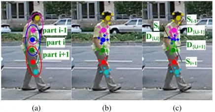
(a) (b) (c)
Figure 2: (a) Parts initialisation. (b) Training samples ob-tained around each part. (c) Implicit shape model. Three regressors estimate one part’s location, each trained using features from samples around different parts.
3.2. Implicit Shape Model
The direct displacement prediction method provides the unique opportunity to combine local information from mul-tiple parts, something not possible with local fitness meth-ods. Consider part i and its neighbours part i −1 and part i+ 1 (see Fig. 2). When seeking to locate part i
we train three separate regressors using image information fromSi−1,SiandSi+1respectively (see Fig.2). Similarly,
in the testing stage we use samples around initial candidate locations of parti−1, partiand parti+1to predict the loca-tion of parti. In this way, the spatial relationships between neighbouring parts are implicitly learned and applied.
Modelling groups of three parts in this way balances lo-cal and global shape. A given part’s movements are closely correlated with its neighbours’, while state changes in far away parts are less likely to affect the given part’s. By com-bining our target parts in overlapping groups of three, these local shape relations effectively create a global shape model (see Fig. 2). Using image information from multiple parts also helps to avoid over-fitting. This embedding of an im-plicit shape model in a set of regressors is only possible because we use direct displacement prediction for tracking. Template matching approaches require the shape to be made explicit in the appearance model.
3.3. Cascaded Linear Regression Tracker
In our implementation of displacement prediction by regres-sion, we adopt a cascaded linear regression framework [22], which was proposed to locate facial landmarks. Crucially, our method is not trained offline as in [22], but is initialised based on the part locations marked in frame 0. We de-scribe the cascaded linear regression framework used in our tracker here.
When training for a given imageIand initial part loca-tionsL∗,Msamples are obtained for each part by randomly
sampling from a relatively close area around the part’s lo-cationl∗i. Sampling locations around partiare denoted as
Si = [si1, ...sij, ...siM]T wheresij is a 2D location in the
image,sij = (xij, yij). The local featuresΦ(I, Si)are
ex-tracted from square patches centred atSi.
We define the displacement vector (our learning goal) to be the vector fromsijtoli∗withd∗ij = (x∗i−xij, yi∗−yij).
The set of all displacement vectors corresponding to M
samples inSi isD∗i = [d∗i1, ..., d∗ij, ...d∗iM]T. That is,Di∗
is the set of displacements fromSi tol∗i. To avoid
confu-sion, we refer toD∗i asDi,i∗ , so thatDi,i∗+1 represents the displacements fromSi+1tol∗i. This is how local shape is
learned.
As we describe in section3.2, we combine three groups of samples to predict parti’s location, which means we use the features fromSi−1,SiandSi+1and their
correspond-ing displacementsD∗i,i−1,D∗i,iandDi,i∗+1to train three re-gressorsRi,1,Ri,2andRi,3 for parti. The trained
regres-sors are able to map the samples’ local featuresΦ(I, Si−1),
Φ(I, Si)andΦ(I, Si+1) to the ground truth displacement
vectorsDi,i∗−1,D∗i,iandD∗i,i+1, which means that the local evidence of all three sets of samples can be used to predict a single target part’s location.
The regressor is obtained by minimising the difference between the predictions and the ground truth. For example, the loss functions forRi,1,Ri,2andRi,3of partiare:
||Di,i∗−1−Ri,1Φ(I, Si−1)||, (1)
||D∗i,i−Ri,2Φ(I, Si)||, (2)
||D∗i,i+1−Ri,3Φ(I, Si+1)||, (3)
and the regressors are obtained by minimising these loss functions. In the following text, we refer to the group of
Ri,1,Ri,2andRi,3asRi. It is hard to find the optimal
pre-diction of the direct displacement in one step [22]. There-fore, we learn the displacement in a cascade of steps with decreasing distance to the target. The cascaded linear re-gression method [22] first learnsR0
i, where0 denotes the
first level of the cascaded regression. Similarly, D0∗
i
de-notes the displacements used for trainingR0
i. We obtainR0
by:
arg min
R0 i,1
||D0i,i∗−1−R0i,1Φ(I, Si0−1)||+||ω||2, (4)
arg min
R0 i,2
||D0i,i∗−Ri,02Φ(I, Si0)||+||ω||2, (5)
arg min
R0 i,3
||D0i,i∗+1−R0i,3Φ(I, Si0+1)||+||ω||2, (6)
where||ω||2is the regularisation term. Please note that we
train each regressor with its corresponding samples and dis-placements. After one cascaded level, we obtainR0and can
[image:4.612.60.278.81.195.2]neighbouring parts’ predictions as follows:
Si1= (Si0−1+R0i,1Φ(I, Si0−1))
∪(Si0+R0i,2Φ(I, Si0))
∪(Si0+1+Ri,03Φ(I, Si0+1)), (7)
whereS1
i is the first cascade level prediction of parti. We
similarly obtain first level predictions of all other parts. Like the first level cascaded regression, R1i,1, R1i,2 and
R1
i,3are obtained by minimising functions4,5,6withS1i−1, S1
i andSi1+1and their corresponding displacementsD1i,i∗−1, D1∗
i,iandDi,i1∗+1. TheR2,R3,... are learned in the same way.
In the test stage, the same number of cascaded regres-sors contribute to the final target location predictionSn
testi,
in whichn is the number of cascade levels. We use Lo-cal Evidence Aggregation for Regression (LEAR) [14] as a principled way of combining the individual evidences. In LEAR, each prediction contributes a unit two-dimensional Gaussian with a fixed standard deviation. LEAR then ag-gregates all these predictions into an un-normalised likeli-hood map of the target’s location. The peak value of this likelihood distribution determines parti’s position.
3.4. Cascaded Incremental Learning
One of the challenges of visual tracking is that ground truth templates, or in our case ground truth direct displacements, are available only for the first frame. Yet the appearance of tracked parts is likely to change over time, especially for deformable objects. The problem is then to decide when and how to update our appearance model (i.e. regressors) without succumbing to the model drift problem.
We use incremental learning [17] as our regressor update method. As described in3.3, the prediction of cascaded re-gression results in a summation of unit Gaussians, one for every prediction made. To estimate the confidence we have in the final prediction, we divide the peak value of the like-lihood map of each part by the total number of predictions. The new peak value is used to evaluate the goodness of our predictions. If it is greater than a thresholdδv, we say that
our predictions are densely distributed. Thus, we are con-fident about our predictions and this tracking result can be used to update our regressors.
Turning the update of cascaded regression into cas-caded incremental learning is non-trivial due to the inter-relationships between the cascades: if the top-level regres-sor improves, this would change the training of all subse-quent steps in the cascade. Asthana et al. proposed a so-lution to cascaded incremental learning for the problem of face alignment [1]. We follow a similar idea to learn the cascade models on the fly and combine the method with our implicit shape model to update the image information and the shape model at the same time. We however found that
using a sequential incremental update provides better results than the specific incremental learning approach of [1].
We minimise Eqs. (4)-(6) to obtainR0i,1,R0i,2andRi,03. For brevity we useX0
i−1to denoteΦ(I, Si0−1). R0i,1,R0i,2
andR0i,3can be estimated by Ridge Regression [10]:
R0i,1= [(Xi0−1)T(Xi0−1) +λE]−1(Xi0−1)TD0i,i∗−1, (8)
R0i,2= [(Xi0)T(Xi0) +λE]−1(Xi0)TDi,i0∗, (9)
R0i,3= [(Xi0+1)T(Xi0+1) +λE]−1(Xi0+1)TDi,i0∗+1, (10)
where E is the identity matrix which is added to make
XTX numerically stable.
As derived in [1], given the feature matrixX(A)and dis-placement matrixD(A), whereAis the number of training samples,R(A)is obtained by:
R(A) =V(A)X(A)TD(A), (11)
V(A) = [X(A)TX(A) +λE]−1, (12)
then withBnew training samplesX(B)and corresponding displacement matrixD(B)obtained from the local neigh-bours and a given part tracked with high confidence, the updated regressorR(A+B)can be found as:
R(A+B) =R(A)−QR(A)+
V(A+B)X(B)TD(B), (13)
where,
V(A+B) =V(A)−QV(A), (14)
Q=V(A)X(B)TU X(B), (15)
U = [E+X(B)V(A)X(B)T]−1. (16)
Note that the new samples added for the update of each part during incremental learning are collected around three parts at each cascade level. In this way the shape and ap-pearance aspects of the regressors models are jointly up-dated, making our tracker robust to the non-rigid deforma-tion of articulated objects.
3.5. Multiple Temporal Scale Motion Model
We add a multiple temporal scale motion model to our regression based tracker, which makes our method a full tracker instead of ’tracking by detection’. As we will show in the results section, displacement based regression works well when test locations are sampled relatively close to the target. Therefore, a good initial estimation of the target po-sition is expected to significantly help to provide accurate final predictions of target position.
motion models from different temporal scales of the target tracking history (i.e. already tracked frames), and applies those models at different temporal scales in the future (see Fig. 3). Here, a temporal scale is a specific sequence of moments in time e.g. [t−4 : t]. The construction of mo-tion models over different temporal scales provides a much richer description of the target’s recent path across the im-age plane. When making predictions, the model set rep-resents variations in target motion better than any single model of this set. The application of these models over multiple temporal scales in the future allows a tracker to overcome periods of occlusion of the object.
0-order motion model
t
t-4 t+1 t+T
Prediction scale
[image:6.612.66.272.234.327.2]Model scale
Figure 3: Multiple motion models are learned from the re-cent tracking history at different temporal scales, and each model is applied over multiple temporal scales in the future.
Simple motion models M are learned over multiple model-scales and are used to make state predictions over multiple prediction-scales, by fitting a first-order polyno-mial function. M is learned at a given model-scale sepa-rately for thex-location, andy-location of the target’s state and M is of order 1. For instance, anMlearned at model-scalem, predicts a target’sx-location at timetas:
˜
xt=βom+β m
1 t, (17)
whereβ1is the slope, andβothe intercept. Model
parame-ters can be learned inexpensively via weighted least squares. A set of learnt motion models at time t is denoted as
[M1
t,M2t, ...,M
|Mt|
t ], where|.|is the cardinality of the set,
which is the number of model scales. In our case, it’s fixed to 4. Each model predicts target state l(˜x,y˜) at T
prediction-scales. After applying the|Mt|models overT
prediction-scales,Tsets of motion predictions are available at timet.
In our part-based tracking approach, a separate MTS mo-tion model is learned independently for each part. The
T × |Mt|motion predictions together with the prediction
of the 0-order motion model, i.e. the predicted location at timet−1, are available at timet. The top ranking motion model is used to initialise the regression search, where the ranking is determined by a classifier trained to distinguish between foreground and background patches.
4. Evaluation
We evaluate our proposed method of part-based tracking by regression with incrementally learned cascades (TRIC) with five experiments: four internal experiments designed to op-timize the parameters for TRIC, and one experiment com-paring TRIC with the state-of-the-art trackers, in which we retrofit a bounding-box around our tracked parts to be able to compare it with bounding-box ground truth.
The dataset used for evaluation of the TRIC tracker in the external experiment is the full dataset of [21]. It in-cludes 50 video sequences and 29 state-of-the-art trackers. This benchmark provides videos with challenging condi-tions such as scale variation, occlusion, deformation, fast motion and so on. Thus, we can avoid over-fitting to a small subset or one specific attribute. All videos are manu-ally tagged with what the main challenges of the video are. For example, DEF is a subset containing all videos with the attribute ‘deformation - non-rigid object deformation’ [21]. OCC is a subset including all videos with the attribute ‘oc-clusion’. SV is the subset in which the videos have ‘scale variation’. The internal studies are performed on 19 videos of the DEF set. We tune the parameters with the subset and then test on the full dataset to avoid over-fitting.
The performance of the various trackers is measured us-ing precision [2,9,21] and success plots. The precision plot measures ‘the percentage of frames whose estimated loca-tion is within the given threshold distance of the ground truth’ [21]. The success plot measures the percentage of frames for which the overlap divided by the union of the predicted and ground truth bounding boxes exceeds a given threshold ratio which varies from 0 to 1. We report on one-pass evaluation (OPE), i.e. the tracker is run throughout the whole video initialised only with the ground truth in the first frame. To rank the performance, as in [21], we use the pre-cision obtained for a location error threshold of 20 pixels as the precision score for the precision plot. For the success plot, the area under curve (AUC) is used.
Because we predict the location of the target directly, and TRIC is a part-based tracker, for the comparison with the state-of-the-art or TRICs with different parameters, we retro-fit a bounding box. This is the same height and width as the bounding box ground truth in the first frame, and its centre location defined as the mean location of all parts.
4.1. Parameters
For calculation efficiency, we re-scale images using the ini-tial frame as the reference to make every tracked target’s scale approximately equal to30×30pixels. Specifically, the ratio is determined by(30∗2)/(w+h), wherewandhare the bounding box groundtruth of the target. The local ap-pearance descriptorΦ(I, Si)used in our implementation is
di-0 10 20 30 40 50 0
0.1 0.2 0.3 0.4 0.5 0.6 0.7 0.8
Location error threshold
Precision
Precision plots of OPE
TRIC(Sample Number=60) TRIC(Sample Number=90) TRIC(Sample Number=120) TRIC(Sample Number=240)
(a)
0 10 20 30 40 50
0 0.1 0.2 0.3 0.4 0.5 0.6 0.7 0.8
Location error threshold
Precision
Precision plots of OPE
TRIC(Radius=15pixels) TRIC(Radius=20pixels) TRIC(Radius=25pixels)
(b)
0 10 20 30 40 50
0 0.1 0.2 0.3 0.4 0.5 0.6
Location error threshold
Precision
Precision plots of OPE
Regression−based Template−based
(c)
0 10 20 30 40 50
0 0.1 0.2 0.3 0.4 0.5 0.6 0.7 0.8
Location error threshold
Precision
Precision plots of OPE
TRIC(Lambda=0) TRIC(Lambda=0.0001) TRIC(Lambda=0.001) TRIC(Lambda=0.01) TRIC(Lambda=0.1) TRIC(Lambda=1) TRIC(Lambda=10) TRIC(Lambda=100) TRIC(Lambda=1000)
(d)
Figure 4: (a) The effect of samples number to the tracking accuracy of TRIC (sampling radius 20 pixels).(b) Effect of sampling radius of TRIC. (c) Comparison between template-based tracker and regression-based tracker. (d) Effect of regu-larisation parameter in ridge regression. The metric in (a),(b), (c) and (d) is the precision plot.
mensionality of the resulting feature space is relatively high, while the number of training samples is limited, we apply principal component analysis (PCA) to reduce the dimen-sionality of the feature. This is also helpful for avoiding over-fitting. Each sample’s HOG feature is represented by
Φ(I, sij, ps, b)in whichbis the bias.
As the object is expected to move, image information acquired from the background will only give approximately correct predictions in the future, while image information derived from the object itself is expected to remain accu-rate over time. Thus, image patches should ideally always capture part of the foreground, which means the size of image patch is approximately equal to the implicit target part’s size. The image patch sizepsis therefore defined by:
ps= (ws+hs)/(N−1), in whichwsandhsare scaledw
andh. This definition ensures that the patch size is directly related to the density of target parts.
N = 6parts are used, as this value represents a balance between shape expressivity and computational complexity. All experiments use fixedδv = 0.0027andM = 90. The
sampling radius is set to 20 pixels and the number of cas-cade levels is 4. In our case, ps is 13 pixels. We set
λ= 0.001 in the Eq. in Sec. 3.4. The number of image feature dimensions kept after PCA is 30.
4.2. Internal Evaluation
The internal tests are performed to optimise the internal pa-rameters of the cascaded regressors. The first internal study examines the influence of the sampling density used in the training and test stages. The second investigates the ef-fect of the sampling radius. The third internal study com-pares the performance of direct-displacement prediction by regression with a template based tracker using the same features and motion model, to investigate the cascaded re-gression’s advantage over the template based method. The fourth internal study evaluates the effect of lambda in the ridge regression. The first, second and fourth experiments are performed with the full TRIC tracker. For the third
experiment, we compare the TRIC tracker, not using the multi-temporal scale motion model and updating, with the template based tracker which uses the same features and motion model (a 0-order motion model).
First, we investigate the effect of sampling density by setting the number of samples to 60, 90, 120, and 240 with the sampling radius fixed to 20 pixels. The results are shown in Fig.4a. The general trend clearly shows that there is not a large difference in the performance of TRIC with sample number either 60 or 90. We choose 90 as the sample number because it is more accurate within smaller error threshold.
Second, the effect of the sampling radius is determined by varying its value in the range of 15, 20 and 25 pixels (see Fig.4b). The results clearly show that a large sampling area is more likely to include poor samples and small one is not robust enough. 20 pixels is selected to balance the accuracy and robustness of the tracker.
Third, for the comparison between the regression-based tracking method and the template-based method, we allow the latter to perform a full search in the same area from which the former samples its test locations, i.e. a circular area of radius 20 pixels. Fig. 4c clearly shows the gain achieved by adopting a regression based approach.
Fourth, we exploit the effect ofλin the Ridge Regres-sion by setting the value ofλto 0 and10k,k = −4 : 3.
Following examination of the results shown in Fig. 4d, we choseλ= 0.001as the optimal value.
4.3. External Evaluation
[image:7.612.66.532.78.186.2]Table 1: Performance of TRIC, without implicit shape model (TRIC-S), without incremental learning (TRIC-I), and without motion model (TRIC-M), on the DEF, OCC, SV and full dataset of the CVPR 2013 benchmark data. # is the rank obtained against the 29 trackers in the benchmark [21], while Score is the precision score.
Trackers TRIC TRIC-S TRIC-I TRIC-M
Dataset # Score # Score # Score # Score
ALL 1 0.752 22 0.470 11 0.527 2 0.691
DEF 1 0.726 18 0.446 11 0.484 2 0.640
OCC 1 0.720 22 0.427 15 0.480 2 0.644
SV 1 0.695 19 0.464 13 0.480 3 0.648
the TRIC tracker without the implicit shape model. Results are shown in Fig.5for precision plot and Fig.6
for the success plot. For clarity, only the top ten trackers are displayed. The values of the two scores for corresponding methods are included in the legends of Fig.5and Fig.6.
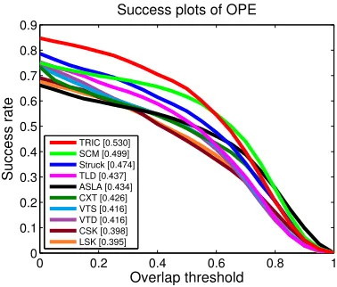
The precision plot of TRIC tracker is about equal to the third-highest ranked tracker (SCM [26]) for a threshold up to 5 pixels, and for higher thresholds it significantly outper-forms all other trackers. Struck [8] comes second. Simi-larly, TRIC clearly outperforms all other trackers for over-lap thresholds up to 0.59, and is approximately equal to SCM after that. One interpretation of these results is that TRIC is a robust tracker, never making very large errors, but not particularly precise. We present another interpretation, and this is that the retro-fitting of a bounding box onto the tracked parts of an articulated deformable object is unsuit-able for direct comparison with bounding box trackers, as deformations of extremities (e.g. someone extending their arm) causes the mean location of the parts to move away from where the bounding box ground truth would be.
Furthermore, Table1shows the precision score, as well as the precision plot ranking obtained, for TRIC, TRIC-S, TRIC-I, and TRIC-M. This clearly shows the value of the implicit shape model. For DEF, without the implicit shape model, performance decreases by 28%. For OCC, perfor-mance decreases by 29% without incremental learning, in-dicating that the incremental learning is crucial for scenar-ios with occlusions, and 10% without the motion model, as the motion model employed by TRIC predicts multiple frames ahead, thus overcoming brief occlusions.
5. Conclusion
We propose a part-based tracker employing direct displace-ment prediction rather than the traditional local matching of an appearance model. The method employs cascaded re-gression to directly predict parts’ locations from local image information, learning the inference models on-the-fly.
Spa-0 10 20 30 40 50
0 0.1 0.2 0.3 0.4 0.5 0.6 0.7 0.8 0.9
Location error threshold
Precision
Precision plots of OPE
[image:8.612.325.515.70.232.2]TRIC [0.752] Struck [0.656] SCM [0.649] TLD [0.608] VTD [0.576] VTS [0.575] CXT [0.575] CSK [0.545] ASLA [0.532] LOT [0.522]
Figure 5: Precision plot of OPE for all 50 sequences.
0 0.2 0.4 0.6 0.8 1
0 0.1 0.2 0.3 0.4 0.5 0.6 0.7 0.8 0.9
Overlap threshold
Success rate
Success plots of OPE
[image:8.612.60.275.154.236.2]TRIC [0.530] SCM [0.499] Struck [0.474] TLD [0.437] ASLA [0.434] CXT [0.426] VTS [0.416] VTD [0.416] CSK [0.398] LSK [0.395]
Figure 6: Success plot of OPE for all 50 sequences.
tial relationships between parts are captured implicitly by a set of regressors. We integrate a multiple temporal scale motion model to initialise our cascaded regression search close to the target and to cope with occlusions. Experi-mental results clearly demonstrate the value of the method’s component parts, and comparison with the state-of-the-art techniques in the CVPR 2013 Visual Tracker Benchmark show that TRIC ranks first on the full dataset.
Acknowledgement
[image:8.612.326.515.276.437.2]References
[1] A. Asthana, S. Zafeiriou, S. Cheng, and M. Pantic.
Incre-mental face alignment in the wild. InComputer Vision and
Pattern Recognition, 2014.2,5
[2] B. Babenko, M.-H. Yang, and S. Belongie. Robust
ob-ject tracking with online multiple instance learning. Pattern
Analysis and Machine Intelligence, IEEE Transactions on,
33(8):1619–1632, Aug 2011.6
[3] T. F. Cootes, G. J. Edwards, and C. J. Taylor. Active
appear-ance models. InComputer Vision - ECCV’98, 5th European
Conference on Computer Vision, Freiburg, Germany, June
2-6, 1998, Proceedings, Volume II, pages 484–498, 1998.2
[4] D. Crandall, P. Felzenszwalb, and D. Huttenlocher. Spatial priors for part-based recognition using statistical models. In
Computer Vision and Pattern Recognition, 2005.3
[5] N. Dalal and B. Triggs. Histograms of oriented gradients for
human detection. InComputer Vision and Pattern
Recogni-tion, pages 886–893, 2005.6
[6] L. Ellis, N. Dowson, J. Matas, and R. Bowden. Linear regres-sion and adaptive appearance models for fast simultaneous
modelling and tracking. Int’l Journal of Computer Vision,
95(2):154–179, 2011.3
[7] P. F. Felzenszwalb, R. B. Girshick, D. McAllester, and D. Ra-manan. Object detection with discriminatively trained
part-based models. Trans. on Pattern Analysis and Machine
In-telligence, 32(9):1627–1645, 2010.3
[8] S. Hare, A. Saffari, and P. Torr. Struck: Structured output
tracking with kernels. InInt’l Conf. Computer Vision, pages
263–270, 2011.3,8
[9] J. a. F. Henriques, R. Caseiro, P. Martins, and J. Batista. Ex-ploiting the circulant structure of tracking-by-detection with
kernels. InProceedings of the 12th European Conference on
Computer Vision - Volume Part IV, ECCV’12, pages 702–
715, Berlin, Heidelberg, 2012. Springer-Verlag.6
[10] A. E. Hoerl and R. W. Kennard. Ridge regression: Biased
es-timation for nonorthogonal problems.Technometrics, 12:55–
67, 1970.5
[11] M. H. Khan, M. F. Valstar, and T. P. Pridmore. Mts: A mul-tiple temporal scale tracker handling occlusion and abrupt
motion variation. InAsian Conf. on Computer Vision, 2015.
2,5
[12] J. Kwon and K. M. Lee. Highly nonrigid object tracking via
patch-based dynamic appearance modeling. Trans. on
Pat-tern Analysis and Machine Intelligence, 35(10):2427–2441,
2013.3
[13] B. Leibe, A. Leonardis, and B. Schiele. Robust object
detec-tion with interleaved categorizadetec-tion and segmentadetec-tion. Int’l
Journal of Computer Vision, 77:259–289, 2008.3
[14] B. Martinez, M. Valstar, X. Binefa, and M. Pantic. Local evi-dence aggregation for regression based facial point detection. Transactions on Pattern Analysis and Machine Intelligence,
35(5):1149–1163, 2013.2,3,5
[15] E.-J. Ong and R. Bowden. Robust facial feature tracking us-ing shape-constrained multiresolution-selected linear
predic-tors. IEEE Trans. Pattern Anal. Mach. Intell., 33(9):1844–
1859, 2011.3
[16] I. Patras and E. R. Hancock. Coupled prediction
classifica-tion for robust visual tracking. Trans. on Pattern Analysis
and Machine Intelligence, 32(9):1553–1567, 2010.3
[17] D. A. Ross, J. Lim, R.-S. Lin, and M.-H. Yang. Incremental
learning for robust visual tracking.Int’l Journal of Computer
Vision, 77(1-3):125–141, 2008.5
[18] S. Shahed Nejhum, J. Ho, and M.-H. Yang. Visual tracking
with histograms and articulating blocks. InComputer Vision
and Pattern Recognition, 2008.3
[19] I. Tsochantaridis, T. Joachims, T. Hofmann, and Y. Al-tun. Large margin methods for structured and interdependent
output variables. Journal of Machine Learning Research,
6:1453–1484, 2005.3
[20] O. Williams, A. Blake, and R. Cipolla. Sparse bayesian
learning for efficient visual tracking.Trans. on Pattern
Anal-ysis and Machine Intelligence, 27(8):1292–1304, 2005.3
[21] Y. Wu, J. Lim, and M.-H. Yang. Online object tracking: A
benchmark. In Computer Vision and Pattern Recognition,
2013.2,6,7,8
[22] Xuehan-Xiong and F. De la Torre. Supervised descent
method and its application to face alignment. InComputer
Vision and Pattern Recognition, 2013.2,3,4
[23] M. Yang, J. Yuan, and Y. Wu. Spatial selection for attentional
visual tracking. InComputer Vision and Pattern Recognition,
2007.3
[24] R. Yao, Q. Shi, C. Shen, Y. Zhang, and A. van den Hengel. Part-based visual tracking with online latent structural
learn-ing. InComputer Vision and Pattern Recognition (CVPR),
2013 IEEE Conference on, pages 2363–2370. IEEE, 2013.3
[25] L. Zhang and L. van der Maaten. Structure preserving object
tracking. InComputer Vision and Pattern Recognition, pages
1838–1845, 2013.3
[26] W. Zhong. Robust object tracking via sparsity-based
collab-orative model. InProceedings of the 2012 IEEE Conference
on Computer Vision and Pattern Recognition (CVPR), CVPR ’12, pages 1838–1845, Washington, DC, USA, 2012. IEEE
Computer Society.8
[27] K. Zimmermann, J. Matas, and T. Svoboda. Tracking by
an optimal sequence of linear predictors. Trans. on Pattern