Lévy Defects in Matrix-Immobilized J Aggregates:
Tracing Intra - and Inter-Segmental Exciton Relaxation
-SUPPORTING
INFORMATION-Larry Lüer*a, Sai Kiran Rajendranb,c, Tatjana Stoll,b Lucia Ganzer,b Julien Rehaultb,d, David M. Colese, David Lidzeye, Tersilla Virgili,b and Giulio Cerullob
a) IMDEA Nanociencia, C/Faraday 9, 28049 Cantoblanco (Madrid), Spain, * larry.luer@imdea.org
b) IFN-CNR, Dipartimento di Fisica, Politecnico di Milano,Piazza L. da Vinci 32, 20133 Milano, Italy
c) School of Physics and Astronomy, University of St. Andrews, St. Andrews, Fife, KY16 9SS (UK)
d) Paul Scherrer Institut, 5232 Villigen PSI, Switzerland
e) University of Sheffield, Department of Physics and Astronomy, Sheffield S3 7RH (UK)
TABLE OF CONTENTS:
A Calculation of exciton states in linear J aggregates with heavy tail states B Calculation of linear absorption and 2DES maps
C Comparison of models
D Complete results of global fitting E Pump intensity dependence F Details of experimental method
A Calculation of exciton states in linear J aggregates with heavy tail states
We consider the single TDBC molecules as two-level systems. Our J aggregate is formed by linearly aligning N of such molecules such that in a Cartesian coordinate system, the position of the nth molecule is [xn; 0; 0]. In the basis of the molecular states |0
⟩
and |n⟩
(all molecules in electronic ground state and nth molecule in excited state, respectively), the Frenkel Hamiltonian reads asH=
∑
n N
ϵnBn†B
n+
∑
n ,m=1;n≠mN
JnmBm† B
n (S1)
Here, Bn†is the creation operator acting on molecule n such that Bn†|0
⟩
=|n⟩
and Bn†|n⟩
=|0⟩
,because it is a two-level molecule, where excitations behave as bosons. Conversely, Bnis the annihilation operator for molecule n acting as Bn|0
⟩
=|0⟩
and Bn|n⟩
=|0⟩
. The parameter ϵnexplicitly consider non-nearest neighbor couplings, which is important to correctly calculate transitions between the one-and two-exciton bands that cause the induced absorption contribution to the two-dimensional spectra (see Fig.1 of main text). Note also that we neglect biexciton stabilization, i.e. we only consider the coupling between singly excited states on the aggregate.i
Diagonal disorder is induced into the Hamiltonian in the following way: for a given aggregate of N monomers, we pick the site energies εn from a set of normally distributed random numbers. The coupling parameters Jnm are calculated from the distance Rn,m of monomers n and m using the point-dipole approximation:
Jnm=ke
[
(μn⋅μm)|Rn , m|
3 −3
(Rn ,m⋅μn)⋅(Rn , m⋅μm) |Rn ,m|
5
]
(S2)with ke=(4π ϵrϵ0)
−1, where
ϵ0=8.854×10
−21F/nm is the dielectric constant in vacuum, and ϵr=3has been assumed for the relative permittivity. The molecular transition dipole moments
μi=μj=[1.869×10⁻²⁰Cm ;0;0]are given as vectors in Cartesian coordinates. For pure diagonal
Gaussian disorder, the position of the aggregate in space is given by {R1=[0,0,0]; Rn,n+1 = [1.0 nm; 0; 0] for n∈{1;..; N−1}}. These numbers were chosen such as to reproduce the experimental red shift of the J aggregate band against the monomer transition.
Off-diagonal disorder is introduced in the following way: We randomly picked a set of Ntr trap positions tj; j∈{1;2;...; Ntr};tj∈{1;2;..; N} along the chain and increased the nearest-neighbor distance at these positions to Rtj,tj±1=
[
±1.2nm;0;0]
. Example: a choice of tj={3;8}on a 10-mer (corresponding to Ntr=2; N=10) would cause the x coordinates of the monomers to be at xn = {0; 1.0; 2.2; 3.4; 4.4; 5.4; 6.4; 7.6; 8.8; 9.8}. Our two traps have thus increased the total length of the 10-mer by 0.8 nm, because the extra distance of 0.2 nm has been applied to the left and to the right at both trap positions. As eq. (S2) is a sharp function of distance, applying an extra distance of only 0.2 nm causes a substantial drop of the intermolecular couplings, leading to an effective segmentation of the aggregate chain. A typical realization of diagonal and off-diagonal disorder can be found in Fig. 1b and c, respectively. Within our model the nearest neighbor couplings Jn,n∓1 can adopt two different values, the “ideal one” and a largely reduced one in the vicinity of the defects. This is an extreme representation of a “heavy tailed” distribution in the sense that the reduced values of Jn,n∓1 in the neighborhood of a trap constitute the “tail” of the (delta-like) distribution of the majority of ideal coupling strengths.For ensemble averaging, we calculated 500 realizations of such aggregates and diagonalized the resulting Hamiltonians using the QuTIP package, restricting the solution space to singly (for simulation of linear absorption spectra) and up to doubly (for simulation of 2DES maps) excited aggregates using excitation number restricted operators. The resulting eigenstate coefficents cem for the singly excited excitonic states e, in the basis of the molecular eigenstates, define the one-exciton wavefunctions:
Ψe=
∑
mcemBm†|0
⟩
(S3)Φf=
∑
kl k>l
Cf ,klBk†B l †
|0
⟩
(S4) [image:3.595.61.539.190.336.2]Note that although the two-exciton coefficients in eq. (S4) carry three indices f, k, and l, they still address elements of the 2D matrix of eigenstate coefficients from the diagonalization of the Hamiltonian, only that in the case of two-excitons, the corresponding doubly excited states (a single column in the C matrix) carry two indices, indicating which molecular excitations are involved.
Figure S1. a) . (a) GSA spectrum (dots) and best fit (solid and dashed line for 70-mer and 35-mer, respectively). b) b) squared error (in a logarithmic color scale) between simulated and experimental GSA spectra as function of the width of the Gaussian distribution of site energies and the number of defects on a 70-mer. C) disorder model deployed for the simulations. Note that for the sake of clarity, only the nearest neighbor coupling Jn,n∓1 is shown while in the calculations also non-nearest neighbor
interactions are included.
B Calculation of linear absorption and 2DES maps
For the calculation of the linear and third order nonlinear spectra, we calculated the linear and third order nonlinear polarization in the impulsive limit, considering all Liouville pathways that survive the rotating wave approximation. However, for the calculation of induced absorption, we found it sufficient to calculate only the 200 lowest energetic two-excitons for each one-exciton state.ii
For this reason, here we pursue a different approach. For each exciton state e, we calculate only those Liouville pathways that do not involve energy transfer. This avoids the time consuming calculation of the Green’s function. What we get is a basis set of pump-probe spectra σ(ω3,ωf)
along ω3 for all f exciton states with energy ωf in the system. The spectral lineshape for the contribution of each Liouville pathway has been calculated using a phenomenological dephasing parameter of Λ=8 meV, which gave best agreement of the tails of experimental and fitted GSA towards low detection energies ω3 (see Fig. S1a). The Beer-Lambert law for a continuous basis set of absorbing species reads as
ΔT/T(ω1,t2,ω3)=−ΔA(ω1, t2,ω3)=ds
∫
ωf
σ( ω3,ωf)⋅D(ω1, t2,ωf)dωf (S5)
where the differential transmission ΔT/T equals the negative of the differential absorption ΔA in the low signal limit, D(ω1, t2, ω3), in units of [cm-3 eV-1], is the exciton distribution function for energies in the range {ωf, ωf +d ωf } at time t2 after excitation with energy ω1 at time t2=0. and the film thickness is given by ds. As we know the pump-probe spectrumσ( ω3,ωf), in units of [cm2],
for all one-excitons, we can find D(ω1,t2,ωf)dωf by a simple non-negative least squares fitting
using the scipy Python package. In order to keep the number of parameters manageable for a nonlinear optimization, we discretized the active space of one-excitons in the range from 2.09 – 2.135 eV into 9 energy bins. This discretization converts the differential density D(ω1,t2,ωf)dωf
into the exciton concentration C [units cm-3] in the energy bin with mean energy ω¯
f:
C( ω1,t2,ω¯f)=
∫
ω=ωf−b/2
ω=ωf+b/2
D(ω1,t2,ωf)dωf (S6)
where b is the width of the energy bins. The concentration-time matrix, finally, is related to the two particle Green’s function by
D(ω1, t2,ωf)=
∑
i
(
D(ω1, t2=0,ωf)⋅G(i , f , t2)
)
(S7)The initial concentrations D(ω1, i, t2=0)of the exciton states can in principle be obtained from
the fit of the linear absorption spectrum and the ω1 spectral distribution.
In a final step, we calculated the transfer matrix (which in the approach of ref[i] is obtained by modified Redfield theory) by solving a system of ordinary differential equations, as implemented in the scipy package, as described in the main text (eq.2).
Here, we highlight the limitations of this approach, introduced by treating exciton dynamics only in a subsequent step. Our approach treats the excited spectrum σ( ω3,ωf) of excitons at energy ωf, as independent of time. In doing so, dephasing effects are not rendered. This might lead to artifacts in the exciton density for very early times (<< 100fs). Moreover, in the calculation of σ( ω3,ωf), the Lorentzian linewidths of all exciton states are all the same, namely the Λ fitting
laptop computer, thus allowing the study of a multitude of samples in which parameters have been systematically varied.
C Comparison of models
In Figure 1 a of the main text, we show that using our model of non-Gaussian off-diagonal disorder, the best agreement between experimental absorption spectrum and simulation is obtained assuming about 6 defects on a 70-mer. Here, we present a more detailed comparison of experimental and simulated spectra using the first four moments. We normalize the integral of
the probe spectrum S(E) to unity, Sn(E)=S(E)/
∫
Emax−0.2eV Emax−0.2eV
Sn(E)dE, E being the probe energy, and Emax being the probe energy of maximum absorption. In order to limit contributions from an incorrect baseline and higher (vibronic or electronic) transitions in the experimental absorption spectrum, we consider only the spectral region close to the absorption maximum in the evaluation of the moments. As the latter depend on these limits, we use the same limits for the moments of the simulated spectra, too. The first momentiii is the mean μ:
μ=
∫
Emax−0.2eV Emax+0.2eV
E⋅Sn(E)dE (S8)
As shown in Fig. S2,the mean µ increases with the number of defects in a roughly linear fashion, while higher amounts of diagonal disorder decrease µ. Note that in Figure S1, the dependence of the mean energy µ on the model parameters has been eliminated by shifting the spectra accordingly to match the simulated µsim with the experimental one, µexp = 2.109 eV.
The second centralized moment is the variance. In Figure S1 b, we show the standard deviation σ, which is the positive square root of the variance:
σ=
(
∫
Emax−0.2eV Emax+0.2eV
(E−μ)2⋅Sn(E)dE
)
1/2
(S9)
The standard deviation is a measure of the width of the band. As Fig. S2b shows, the width rises with increasing number of defects as well as with increasing diagonal disorder. The experimental value, σexp = 0.049 eV, can actually be obtained for any assumed value of defect concentrations or diagonal disorder by adjusting the other one. So the discussion on whether non-Gaussian off-diagonal disorder is needed to reproduce the experimental absorption spectrum, cannot be based on considering only the width of the band. The important figures of merit are the skewness and “tailed-ness” (kurtosis) of the band, which are the third and fourth moments, respectively.
The Pearson’s moment coefficient of skewness is defined as the third standardized moment:
γ=
∫
Emax−0.2eV Emax+0.2eV
(E−μ)3⋅Sn(E)dE/σ3 (S10)
diagonal disorder get closest, attaining skewness values up to 0.85. The reason for the high skewness in the absence of diagonal disorder is the “built-in” skewness of the absorption spectrum of an ideal J aggregate. Although most of the transition strength comes from the lowest energetic exciton state, about 10% derive from higher lying exciton states. The skewness of the band thus depends on the energetic splitting between the lowest and the next higher exciton states, which is a function of exciton delocalization. Therefore, the standardized skewness (skewness of a band that has been scaled to standard deviation one, see eq. S9) decreases with increasing diagonal disorder, because diagonal disorder adds inhomogenous broadening to the band, which acts more strongly on the standard deviation (Fig. S2b) than on the exciton localization (Fig. S2A).
Finally, the fourth standardized moment is the kurtosis or “tailed-ness” of a band:
κ=
∫
Emax−0.2eV Emax+0.2eV
(E−μ)4
⋅Sn(E)dE/σ4
(S11)
According to eq. S10, a Gaussian function attains a kurtosis of κ=3. The kurtosis of the experimental absorption spectrum is κexp = 5.6. In Fig. S2d, we show that several combinations of the model parameters yield this experimental kurtosis. The highest kurtosis is found in the absence of both diagonal and off-diagonal disorder; in this case, the Lorentzian lineshapes dominate the kurtosis, being much stronger tailed than a Gaussian.
Fig. S2. First, second, third, and fourth moments of the simulated linear absorption spectra, using the model of hard segmentation by defects as explained under point A of this supporting material
(panels a,b,c,and d, respectively)
In Fig. S3, we show the result of the simulation of the experimental absorption spectrum by assuming a Lévy distribution of the site energies (diagonal disorder) rather than the couplings (off-diagonal disorder). A symmetric Lévy distribution with mean zero is given byiv
p(E)= 1 2π−∞
∫
+∞
eiEte−(|βt|)α
dt , (S12)
Fig. S3: a) experimental absorption spectrum (dots) and best fit of simulations assuming only diagonal disorder given by a stable symmetric Lévy distribution according to eq. S11 (line). b) The squared error between experiment and simulation, given in a logarithmic color scale (see scale bar) as
function of the Lévy parameters.
D Complete results of global fitting
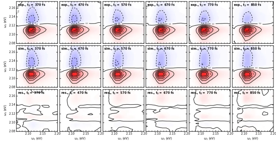
In Fig.S4 a,b, we show experimental 2DES maps at various t2 times up to 200 fs, the corresponding fits according to eq. S6, and the residuals, in the upper, middle and lower row, respectively. In Fig. S5, we show the same graphs for t2 times from 370 fs upward. In Fig.S6, we show the time-resolved exciton densities, as obtained from the fits in Fig.S5 in the upper row, while the middle row shows global fits obtained by numerical integration of a system of ordinary differential equations, after nonlinear optimization has been performed on the transfer matrix elements (eq.4 in main text) . The lower row shows the residuals. Fig. S7 is the same as Fig.S6, but for longer t2 times. Fig. S8 gives the transition dipole moment, density of states, and excited state spectra of one-excitons as function of exciton energy. Figures S9, S10, and S11, finally, show exciton densities C( ω1,t2,ωf) obtained according to eq. 1 in main text, and and fits according to
[image:8.595.133.457.60.223.2]Fig. S4. Experimental 2DES maps, global fits according to eq. S3 using basis states σ(ω3,f) from a Frenkel
exciton model (see Fig. S6), and residuals. (upper, middle , and lower row, respectively)
[image:9.595.79.519.376.604.2]Fig. S6. Time and energy resolved exciton densities C(ω1,i , t2=0), as obtained from the global fits in Fig.S4,
global fits to C( ω1,i , t2=0)by nonlinear optimization of the off-diagonal transfer matrix elements and the
dispersiveness parameter γ in eq.2 in main text, and residuals (upper, middle, and lower row, respectively). The false color scale is defined by the maximum signal in the upper row and valid for all three rows.
[image:10.595.82.518.435.661.2]Fig. S8. A) Normalized transition dipole moment for the basis of one-exciton states from the ground state (black) and normalized density of exciton states per energy interval, as function of one-exciton energy. B) Basis spectra σ(ω3,f) as a function of one-exciton energy, as obtained from calculation of
all relevant Liouville pathways starting from the specific one-exciton, normalized to the PB maximum. These states were obtained by diagonalization of a Frenkel Hamiltonian of an aggregate
containing Gaussian disorder in the site energies but heavy tail states in the coupling. See Fig.S1C for a pictorial representation of the simulated aggregate. The graph shows that the evolution of the
characteristic features of the basis spectra with exciton energy is sufficiently smooth to justify the binning that we have used to reduce the number of basis states in eq. S6.
E Pump fluence dependence
[image:11.595.61.534.62.243.2]We performed the same analysis on various sets of 2DES maps, varying the pump fluence from 0.3 up to 2.1 μJ cm-2. In Fig. S9, we show the values of the 2DES maps at ω1 = ω2 = 2.13 eV (region of photoinduced absorption) for various times t2. Although the pump fluence has been varied by nearly an order of magnitude, the normalized time traces remain very similar. From Fig.S9, we can therefore not confirm the presence of singlet annihilation which has been described in TDBC/water.v
[image:11.595.186.412.555.733.2]For the simulations of the intensity dependent 2DES maps, we used the same set of exciton states as in the evaluation according to eq.1 in the main text. The resulting time-resolved exciton distributions are given in Figs S11-13, upper rows. Fitting these with a rate equation model (eq.2 in main text) was possible without systematic deviations, see middle and lower rows for fits and residuals, respectively. The resulting transfer matrices are shown in Fig. S10. They all show similar features as Fig. 4b in main text, namely matrix elements for downward ET which are orders of magnitude faster than those for upward ET. However, increasing the pump intensity leads to an overall reduction of the matrix elements. This finding might be explained by exciton annihilation, being an energy transfer process between two excitons, yielding one exciton in a hot ground state and the other one in a highly excited state. By this mechanism, high energy excitons are constantly “recycled” as long as there is sufficient exciton population, thus yielding an apparent reduction of the overall exciton relaxation rate.
Fig. S10. Diagonal value kii(t2= 1 ps) of the dispersive transfer matrix that results from the fittings in Fig.S10, S11,and S12, using eq. 2 of main text, as function of exciton energy, for measurements
Figure S11: like Fig. S6; pump energy 0.3 μJ cm-2
[image:13.595.84.519.374.618.2]F Details of Experimental Method:
Two-dimensional electronic spectroscopy was performed in the partial collinear pump-probe geometry employing two collinear phase-locked pump pulses and a non-collinear probe pulse. The probe is delayed by the the population time t2 and its spectrum is measured by a spectrometer. Additionally, a phase-locked pump pulse pair is generated and the two identical pulses are delayed by the coherence time t1. The Fourier transform with respect to t1 allows to resolve the obtained signals with respect to excitation energy. 2DES spectroscopy provides thus the possibility of combining excellent time and spectral precision in excitation and probing.
A broadband non-collinear optical parametric amplifier (NOPA) was used to generate the 10 fs-pump and probe pulses with spectrum spanning the 1.8-2.35 eV range. The NOPA was pumped by 100fs-pulses at 800nm from a regeneratively amplified 1 kHz repetition rate Ti:Sapphire laser (Coherent Libra). To generate coherence delay (T1), a novel optical device, called TWINS, was used, where the birefringence of α-BBO crystals generates variable delays for pulses polarized along the ordinary and extraordinary axes. As shown in Figure S13, the TWINS setup consists of three blocks A, B and C of two birefringent plates and wedges with their optical axes as shown by yellow arrows. A linear polarizer (1) changes the pump beam polarization from vertically (along the X-axis) to a polarization of 45° with respect to the XY plane. The beam passes through block A which consists of two wedges with optical axis along the Z-axis, the direction of propagation; and Y-axis, respectively. Since the horizontal and vertical components of the pump beam propagate with different velocities depending on the different refractive indexes, they are delayed by t1. By moving the entire block A, it is possible to scan delay t1. Due to the different refraction for the X-and Y- pulses at the interfaces, the pulses are not collinear X-and their phase fronts are not parallel after passing through block A. In order to correct these features, block B is inserted in the path. It is composed of two wedges identical to those in block A but placed in the opposite order. Block C, whose optical axis is along the X-axis, introduces a constant negative delay. After passing through the second linear polarizer (2), the two orthogonal and delayed pump pulses are both polarized at 45° with respect to the XY plane.
The birefringent material introduces a positive dispersion to the pump pulses which is compensated by a pair of chirped mirrors. The pump pulses are compressed to near transform limit by adjusting the number of reflections at the chirped mirror pair. The pump pulses then pass through a chopper working at a frequency of 500 Hz.
The t1 delay and phase between the two pump pulses, are calibrated by translating block A and observing the interference fringes of the beams scattered by a pinhole at the sample position into the spectrometer. The pump delay and phase are monitored in parallel to data acquisition and the subsequent t1 scans by deviating a small part of the pump beams into a photodiode and acquiring their interference.
The probe pulse dispersion is compensated by another pair of chirped mirrors. The population delay (t2) between the pump and probe pulses is controlled by another pair of mirrors on a translation stage. The interference between the scattered pump pulses and the probe pulses is minimized by using an audio speaker changing the optical path of the probe beam.
Fig. S14. Experimental set up for 2DES
i Stiopkin, I.; Brixner, T. Yang, M.; Fleming, G. R. Heterogeneous Exciton Dynamics Revealed by Two-Dimensional Optical Spectroscopy, J. Phys. Chem. B 2006, 110, 20032-20037
ii Dijkstra, A. G.; Jansen, T. L. C.; and Knoester, J. Localization and coherent dynamics of excitons in the two-dimensional optical spectrum of molecular J -aggregates, J. Chem. Phys. 2008
128, 164511
iii For the definition of moments, see https://en.wikipedia.org/wiki/Moment_(mathematics)
iv Feller, W. An Introduction to Probability Theory and Its Applications (Wiley, New York, 1966).