DOI 10.1007/s00285-012-0506-0
Mathematical Biology
Limitations of perturbative techniques in the analysis
of rhythms and oscillations
Kevin K. Lin · Kyle C. A. Wedgwood · Stephen Coombes · Lai-Sang Young
Received: 1 October 2011 / Revised: 13 January 2012 / Published online: 31 January 2012 © The Author(s) 2012. This article is published with open access at Springerlink.com
Abstract Perturbation theory is an important tool in the analysis of oscillators and their response to external stimuli. It is predicated on the assumption that the pertur-bations in question are “sufficiently weak”, an assumption that is not always valid when perturbative methods are applied. In this paper, we identify a number of con-crete dynamical scenarios in which a standard perturbative technique, based on the infinitesimal phase response curve (PRC), is shown to give different predictions than the full model. Shear-induced chaos, i.e., chaotic behavior that results from the ampli-fication of small perturbations by underlying shear, is missed entirely by the PRC. We show also that the presence of “sticky” phase–space structures tend to cause perturba-tive techniques to overestimate the frequencies and regularity of the oscillations. The phenomena we describe can all be observed in a simple 2D neuron model, which we choose for illustration as the PRC is widely used in mathematical neuroscience.
Keywords Oscillators·Perturbation theory ·Phase response curve· Neuron models·Shear-induced chaos
Mathematics Subject Classification (2000) 92B25·37N25
K. K. Lin (
B
)Department of Mathematics and Program in Applied Mathematics, University of Arizona, Tucson, AZ, USA
e-mail: [email protected] K. C. A. Wedgwood·S. Coombes
School of Mathematical Sciences, University of Nottingham, Nottingham, UK L.-S. Young
0 Introduction
Rhythmic activity is commonplace in biological phenomena: the spontaneous beating of heart cells in culture (Glass et al. 1984), the synchronization of flashing fireflies (Mirollo and Strogatz 1990), and central pattern generators in animal locomotion (Cohen et al. 1988), and calcium oscillations that underlie a plethora of cellular responses (ranging from muscle contraction to neurosecretion) (Thul et al. 2008) are just a few examples (see, e.g.,Glass and Mackey 1988;Winfree 2000for many more). Mathematical models of biological oscillations often provide useful insights into the underlying biological process; for example, they can explain the observed robustness of circadian rhythms (Winfree 2000) and of population cycles (May 1972), and can be used to infer plausible structures for central pattern generator networks based on locomotion gaits (Golubitsky et al. 1999). Analyzing models of biological oscilla-tions, however, is generally not easy: the mechanisms underlying biological rhythms are varied and complex, and this complexity is reflected in the corresponding mathe-matical models. Indeed, models of biological oscillators are often high dimensional, highly nonlinear, and have uncertain parameters, all of which make them challenging to study.
Perturbation theory, long a staple of applied mathematics, provides a practical solu-tion in many situasolu-tions. Mathematically, robust oscillasolu-tions correspond to attracting limit cycles in phase space. If the stimuli involved are not too strong, then one is justified in viewing trajectories of the forced system as perturbations of the original limit cycle. When judiciously applied, such perturbative analyses can yield a great deal of insight and useful quantitative predictions. For oscillators, a good example of an effective perturbation technique is that of infinitesimal phase response curves (PRCs) and associated phase reductions (Ermentrout and Kopell 1991). The infinitesimal PRC of an oscillator records the phase change that results from an applied perturbation. Given an oscillator, there are many ways to obtain its infinitesimal PRC: in addition to analytical perturbation techniques, there are efficient numerical methods for construct-ing PRCs; the entire PRC itself can even be inferred directly from experimental data. Moreover, PRC-based techniques require only tracking just the phase of the oscillator, thereby greatly reducing complexity. They are used in many areas of mathematical biology, but especially in computational neuroscience, as they yield direct predictions about the modulation of spike timing and frequency by external stimuli. Furthermore, they allow one to make predictions for weakly-coupled networks (Hoppensteadt and Izhikevich 1997;Pikovsky et al. 2001).
near a limit cycle, which can cause perturbation theory to overestimate the regularity and frequency of a stimulated oscillator. We will also show that dynamical shear in a neighborhood of the oscillator can cause it to behave chaotically when forced. These scenarios cannot be captured by infinitesimal phase reductions.
The scenarios described in this paper are relevant for general oscillators, but in view of the popularity of PRC-based techniques in neuroscience, we will illustrate our ideas using the Morris–Lecar (ML) neuron model (Ermentrout and Rinzel 1991;
Ermentrout and Terman 2010). This widely-used model provides a convenient and flexible example because of its low dimensionality and rich bifurcation structure. The phenomena of interest are not hard to find in certain ML regimes; they do not require stringent tuning of parameters. We point out also that while we focus here on single neuron models, our findings remain relevant for oscillators operating within networks. This paper is organized as follows: In Sect.1, we review some relevant mathematical background, including brief discussions of phase response theory and “shear-induced chaos”, a general mechanism for producing chaotic behavior in driven oscillators. Sect.2introduces the ML model and some relevant ideas from computational neuro-science. In the last three sections, certain regimes of the ML model are used to dem-onstrate how perturbative techniques sometimes do not correctly predict the behavior of the full model. Sect.3contains an example in which the infinitesimal PRC gives no hint of the strange attractor in the full model. Sects.4and5illustrate how the presence of nearby invariant structures can impact neuronal response in ways that cannot be captured by PRCs alone.
1 Mathematical background
The general setting for this section is a nonlinear oscillator modeled by an n-dimen-sional ODEx˙ = f(x)with a limit cycleγ. We assume throughout thatγ is not only attractive as a periodic orbit but hyperbolic, i.e., its Floquet multipliers have absolute values<1. The period ofγ is denoted Per(γ ).
1.1 Phase response curves and phase reductions
This section contains a brief review of a perturbation technique for oscillators known as (infinitesimal) phase response theory. For more details and many applications, see, e.g.,Ermentrout and Terman(2010),Glass and Mackey(1988),Guckenheimer(1974),
Winfree(2000).
First, we fix a notion of “phase” on the oscillator: Fix a reference point x∗ ∈ γ, and declare its phase to beψ(x∗)=0.1For any other point x ∈ γ, the phaseψ(x)
can be defined to be the amount of time to go from x∗to x along the cycleγ, i.e., if a solutionηsatisfiesη(0)= x∗,thenη(ψ(x)) = x.Next we extend this notion to a neighborhood ofγ. It is a mathematical fact thatψextends uniquely to a smooth
function such that for all solutions x with x(0)nearγ,dtdψ(x(t))=1. Thusψserves as a kind of “clock” for tracking the passage of time along trajectories nearγ.
Our goal is to describe what happens to the phase when a time-dependent perturba-tion is applied. Letθ(t):=ψ(x(t)), where x is a perturbed trajectory. We would like an approximate equation forθ(t). Rather than doing this for general perturbations, we consider a perturbed equation of the form
˙
x= f(x)+I(t)kˆ, (1)
where x(t)∈Rn, I is a scalar signal, andkˆ ∈ Rn is a constant vector. (In neurosci-ence applications, for example, one of the variables usually represents the membrane voltage, and this is typically the only variable that can be directly affected by external perturbations.) Now letξ :R→Rnbe a periodic solution to the “adjoint equation”
˙
ξ(t)= −D f(γ (t))T ·ξ(t), (2)
whereγ (t)denotes an orbit parametrizing the cycleγ, and letΔ(θ):=ξ(θ)· ˆk. Under
the normalization conditionξ(0)· f(0)=1,2it can be shown (see, e.g.,Ermentrout and Terman 2010) that if x is a solution of Eq. (1) and I =O(ε)for a small parameter
ε, thenθsatisfies
˙
θ=1+Δ(θ)I(t)+O(ε2). (3) Truncating all terms of O(ε2)in Eq. (3) yields an equation forθ, the phase reduction of Eq. (1). The functionΔis the infinitesimal phase response curve (PRC).3
For systems that are near a bifurcation, the above procedure can be used to derive analytical approximations of the PRC via normal forms (Brown et al. 2004). In more general situations (where there are few practical analytical techniques), one can obtain PRCs through numerical computation, or even directly from experimental measure-ments (see, e.g.,Oprisan et al. 2003;Netoff et al. 2005;Winfree 2000and references therein). This flexibility and accessibility is part of its appeal in mathematical biology, and in neuroscience in particular.
Stochastic forcing The basic methodology of infinitesimal phase response curves can
be extended to systems driven by stochastic forcing. That is, suppose that in addition to a deterministic forcing, we add a second white-noise term:
˙
x= f(x)+(I(t)+βW˙)kˆ; W˙ =white noise.
Ly and Ermentrout(2011) show that with the above forcing,θsatisfies the equation
˙
θ=1+Δ(θ)I(t)+β
2 2 Δ(θ)Δ
(θ)+βΔ(θ)W˙ +(higher order terms), (4)
assuming bothεandβare small.
Eq. (4) can be used to derive a number of quantities of interest. For example, if we view Eq. (4) as modeling a neuron that “fires” wheneverθ =0, then a result of Ly and Ermentrout states that the firing rate resulting from a constant forcing I(t)≡εis
r(ε)=1+εΔ¯+ε2 Per(γ )
0
(Δ¯2−Δ2(θ))
dθ
+β4
4 Per(γ )
0
Δ2(θ)(Δ(θ))2dθ+O(ε3), (5)
to leading order inβ. In the above,Δ¯=0Per(γ )Δ(θ)dθ.
Remark on terminology Other variants of the PRC exist for finite-size perturbations.
In this paper, the term “PRC” will always mean the infinitesimal phase response curve.
1.2 When do phase reductions work, and when might they fail?
Because the PRC is defined in terms of a vector field f and its derivative along a limit cycleγ[see Eq. (2)], it can only contain information about the flow in an infinitesimal neighborhood ofγ. We discuss briefly in this subsection a few scenarios in which the behavior of the flow a finite distance away fromγ can have a dramatic effect on the oscillator’s response. These ideas are illustrated in concrete examples in Sects.3–5. (1) Leaving the basin ofγ The simplest possible way for something to go wrong is when the forcing carries a phase point outside of the basin of attraction ofγ. IfΦt
denotes the unforced flow, then the basin ofγ, denoted Basin(γ ), is defined to be the set of all phase points x such thatΦt(x)→γas t → ∞. Once a perturbation, say in
the form of a “kick”, causes a trajectory to leave Basin(γ ), what it does may depend on dynamical structures far away fromγ. For example, if the system is bistable, or multi-stable, i.e., it has more than one attracting set, which can be in the form of a stationary point, a limit cycle, or something more complicated, then an “escaped” tra-jectory can end up near one of these structures, and in time, it may—or may not—get kicked back into Basin(γ ). Needless to say, the behavior of such a trajectory bears little resemblance to that predicted by the PRC. This scenario must be taken into con-sideration when the forcing is strong relative to the distance of∂(Basin(γ ))toγ. [Here
∂(Basin(γ ))is the boundary of Basin(γ ).]
LIMIT CYCLE
KICK
[image:6.439.104.332.64.141.2]S
HEAR
Fig. 1 The stretch-and-fold action of a kick followed by relaxation in the presence of shear
perturbed trajectory that gets near it will likely escape eventually and return toγ. However, the escape time can be quite long, and this effect cannot be captured by phase reductions. The tendency to remain near invariant structures can be mitigated by the forcing when the forcing acts to push trajectories away; by the same token, it can also be magnified if the forcing “conspires” to keep trajectories in a region. Indeed, there is no reason why a forcing cannot—by itself— create trapping regions within the basin ofγif the attraction toγis weak compared to the forcing.
(3) Shear-induced chaos This is yet another dynamical phenomenon that cannot be captured by (infinitesimal) PRCs. This phenomenon is illustrated in Fig.1. In each of the two pictures,γ is represented by the horizontal line. Shear refers to the dif-ferential in the horizontal component of the velocity as one moves vertically up in the phase space; here points aboveγ move aroundγ faster than points below. Sup-pose that an impulsive perturbation, or “kick,” applied in such a situation produces a “bump” in γ. As the flow relaxes, this “bump” is attracted back to the original limit cycle. As it evolves, it is folded and stretched by the flow if sufficient shear is present, as one can visualize in Fig.1. Since stretching and folding of phase space is associated with complex dynamical behavior such as horseshoes and strange attrac-tors (Guckenheimer and Holmes 1983), this picture suggests that perturbing a limit cycle with strong shear can lead to chaotic dynamics. That this can indeed hap-pen has been established (rigorously) in recent developments in dynamical systems theory.
To connect paragraphs (2) and (3), we mention that invariant structures in
∂(Basin(γ ))can be a contributing factor to shear, but shear can also arise for many other reasons. Since the results on shear-induced chaos alluded to above are not widely known in the mathematical biology community, we will provide a more detailed review in the next subsection.
1.3 Shear-induced chaos and related phenomena
In this section, we review some of the geometric ideas put forth inWang and Young
A periodically-kicked oscillator is a system of the form
˙
x = f(x)+A·H(x)
∞
k=−∞
δ(t−kT), (6)
where(A,T)∈R×R+are parameters and H :Rn →Rnis a given smooth func-tion. We assume as before thatx˙ = f(x)has an attracting hyperbolic limit cycleγ. Equation (6) thus models an oscillator that is given a sharp “kick” every T units of time. We interpret the kicks as follows: whenever t = nT , we apply a mappingκ
(defined by H ) to the system; between kicks, the system follows the flowΦt
gener-ated by x˙ = f(x). When kicks are applied repeatedly, the dynamics of Eq. (6) can be captured by iterating the time-T map FT =ΦT ◦κ. If there is a neighborhoodU
ofγ such thatκ(U)⊂Basin(γ ), and T is long enough that points inκ(U)return to
U, i.e., FT(U)⊂U, thenΓ = ∩n≥0FTn(U)is an attractor for the periodically kicked system FT. One can viewΓ =Γ (κ,T)as what becomes of the limit cycleγ when
the oscillator is periodically kicked.
The structure ofΓ and the associated dynamics depends strongly on the kick param-eters A and T , as well as on the relation between the kick mapκ and the flow near
γ. When A is small, we generally expectΓ to be a slightly perturbed version ofγ, because (as is well known) hyperbolic limit cycles are robust under small perturba-tions (Guckenheimer and Holmes 1983). In this case,Γ is known as an invariant
circle, and the restriction of FT toΓ is equivalent to a diffeomorphism on S1. Circle
diffeomorphisms are well known to exhibit essentially two distinct types of behavior:
quasiperiodic motion, in which the mapping is equivalent to rotation by an irrational
angle, and gradient-like behavior characterized by sinks and sources on the invariant circle. In terms of the kicked oscillator dynamics, the former corresponds to the driven oscillator drifting in and out of phase relative to the kicks, while the latter corresponds to stable phase-locking.
The preceding discussion suggests that when kicks are weak, we should expect fairly regular behavior. To obtain more complicated behavior, it is necessary to “break” the invariant circle. The main idea is best illustrated in the following linear shear model, a version of which was first studied inZaslavsky(1978):
˙
θ=1+σy ˙
y= −λy+A·H(θ)·
∞
n=0
δ(t−nT), (7)
where(θ,y)∈ S1×Rare coordinates in the phase space,λ, σ, and A are constants, and H : S1 → Ris a non-constant smooth function. When A = 0, the unforced system has a limit cycleγ =S1× {0}. The following result, due to Wang and Young, shows that Eq. (7) indeed exhibits chaotic behavior under the right conditions. [There is an obvious analog in n-dimensions (Wang and Young 2003).]
Theorem 1 (Wang and Young 2003) Consider the system in Eq. (7). If the quantity
σ λ ·A ≡
shear
is sufficiently large (how large depends on the forcing function H ), then there is a positive measure setΔ⊂ R+such that for all T ∈ Δ, Γ is a “strange attractor” of FT.
It is important that H be non-constant, as H(θ)is what creates the bumps in Fig.1. The geometric meaning of the term involvingσ, the shear, is as depicted in Fig.1. It is easy to see whyσλ·A is key to production of chaos by fixing two of these quantities
and varying the third: the largerσ, the larger the fold; the same is true for larger kick size A. Notice also that weaker limit cycles are more prone to shear-induced chaos: the closerλis to 0, the slowerκ(γ )returns toγ, and the longer the shear acts on it, assuming T is large enough.
The term “strange attractor” in Theorem1is used as short-hand for an attractor with an SRB measure,4which roughly speaking, implies that the trajectory is unstable, or has a positive Lyapunov exponent, starting from Lebesgue-almost every initial condi-tion in the basin of the attractor (or at least in a positive measure set). We say such a system has a “strange attractor” because it exhibits sustained, observable chaos, i.e., chaotic behavior that is sustained in time, and observable for large sets of initial con-ditions. This is a considerably stronger form of chaos than the presence of horseshoes alone (see e.g.Guckenheimer and Holmes 1983for a discussion of horseshoes). In the latter case, it is possible for almost all orbits to end up at stable equilibria, resulting in negative Lyapunov exponents; this scenario, in which horseshoes coexist with sinks, is known as transient chaos.5
Shear-induced chaos and the geometry of strong stable manifolds or isochrons
We now return to the general setting of Eq. (6) and seek to understand what plays the role of the shear (asσ is no longer defined). Letγ andΦt be as at the beginning
of Sect.1.3. Crucial to this understanding is the following dynamical structure of the unperturbed flowΦt: For x ∈γ, define the strong stable manifold or isochron through x to be
Wss(x)= {y: |Φt(y)−Φt(x)| →0 as t→ ∞}.
Withγ assumed to be hyperbolic, it is known that (see, e.g.,Guckenheimer 1974) (i) Wss(x)intersects γ transversally at exactly one point, namely x, and these
manifolds are invariant in the sense thatΦt(Wss(x))=Wss(Φt(x)).
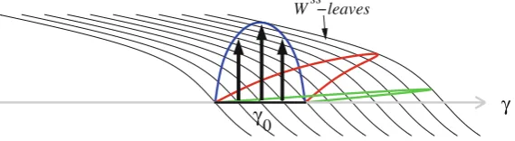
(ii) {Wss(x),x∈γ}partitions Basin(γ )into codimension-1 submanifolds. We now examine the action of the kick mapκ in relation to the Wss-foliation. Figure 2 is analogous to Fig. 1; it shows the image of a segment γ0 of γ under
FT =ΦT ◦κ. For illustration purposes, we assumeγ0is kicked upward with its end points held fixed, and assume T = np for some n ∈ Z+ (otherwise the picture is
4 For more information, seeEckmann and Ruelle(1985) andYoung(2002).
5 Note that Theorem1asserts the existence of “strange attractors” only for a positive measure set of T , not
ss
γ
0W −leaves
[image:9.439.78.363.59.137.2]γ
Fig. 2 Geometry of folding in relation to the Wss-foliation. Shown are the kicked image of a segmentγ0
and two of its subsequent images underΦnp, p=Per(γ )
shifted to another part ofγ but is qualitatively similar). SinceΦnpleaves each Wss
-manifold invariant, we may imagine that during relaxation, the flow “slides” each point of the curveκ(γ0)back towardγalong Wss-manifolds. In the situation depicted, the effect of the folding is evident.
Figure2gives considerable insight into what types of kicks are conducive to the formation of strange attractors. Kicks along Wss-manifolds or in directions roughly parallel to the Wss-manifolds will not produce strange attractors, nor will kicks that essentially carry one Wss-manifold to another. What causes the stretching and folding is the variation in how far points x ∈γare moved byκ as measured in the direction transverse to the Wss-manifolds. In the simple model of Eq. (7), because of the lin-earity of the unforced equation, Wss-manifolds are straight lines with slope −λ/σ in(θ,y)-coordinates. Variation in the sense above is created by any non-constant H ; the larger the ratioσλA, the greater this variation.
The notion of “phases” in Sect.1.1is defined precisely by the partition of neighbor-hoods ofγinto Wss-manifolds or isochrons (two names used by different communities for the same object), i.e., we view x ∈Basin(γ )as having the same phase as y∈γ if x ∈ Wss(y). The ideas in the last paragraph are in the same spirit as the phase
transition curves introduced byWinfree(2000), (see alsoGlass and Mackey(1988) andErmentrout and Terman(2010)). They were discovered independently in the rig-orous work ofWang and Young(2001,2008), who proved, under suitable geometric conditions on phase variations, the existence of strange attractors having many of the properties commonly associated with chaos. These ideas have since been applied to various situations; rigorous results includeWang and Young(2002,2003),Lu et al.
(2012),Ott and Stenlund(2010),Wang and Ott(2011) andDeville et al.(2011), and numerical results indicate the occurrence of shear-induced chaos in broader dynamical settings (Lin and Young 2008;Lin et al. 2009a;Lin 2006).
1.4 Summary and comparisons
Sections1.1and1.3outlined two seemingly distinct approaches to the analysis of phase response. These approaches are in fact closely related: In Sect. 1.1, pertur-bations are assumed to be small, which geometrically means one can approximate
Sect.1.3is a more global version of the same idea: here the perturbed orbit is allowed to wander farther away fromγ, and one takes into consideration the geometry (or curvature) of the Wss-manifolds in relation to the kick in assessing its impact.
A notable difference between full-model analyses and phase reductions is that the latter rule out a priori any possibility of chaotic behavior. As explained in Sect.1.3, in the full model, fairly innocuous kicks applied “the right way” can lead to positive Lyapunov exponents for large sets of initial conditions. This cannot be captured by the infinitesimal PRC, for flows in one spatial dimension are never chaotic.
With regard to practicalities, full model analyses are, needless to say, more costly. While our aim here has been to raise awareness of the issues discussed in Sects.1.2
and1.3, it is not our intention to advocate that one necessarily starts by computing
Wss-manifolds (even though they are computable in many situations). In many cases, by far the most direct way to get a quick idea of whether shear-induced chaos is present is to look at FT-images ofγ(recall that FT =ΦT ◦κis the composite map obtained
by first kicking then following the unperturbed dynamics for time T ) and see if folds develop. See Sect.3.
2 A neuron model
In Sects.3–5, a few concrete scenarios will be presented to illustrate how and why the infinitesimal PRC may give incorrect predictions. The model we use is taken from neuroscience; it is the Morris–Lecar (ML) model of neuron dynamics. A brief intro-duction of the ML model and some relevant information is given below to provide context for readers not familiar with the subject. We remark that perturbation methods and the infinitesimal PRC in particular are widely used in neuroscience, both in the study of single neuron dynamics (see e.g.Ermentrout and Terman 2010) and in the analysis of neuronal networks modeled as systems of coupled phase oscillators (see e.g.Hoppensteadt and Izhikevich 1997).
The Morris–Lecar (ML) model
The dominant mode of communication between neurons is via the generation and transmission of action potentials, or “spikes” (Dayan and Abbott 2001). Neurons accomplish this through the coordinated activity of voltage-sensitive ion channels in the cell membrane, which open and close in specific ways in response to changes in membrane voltage. The ML model is a simple model of this spike-generation process for a single neuron. It has the form
Cmv˙ =I(t)−gleak·(v−vleak)−gK w·(v−vK)−gCam∞(v)·(v−vCa)
˙
w=φ·(w∞(v)−w)/τw(v).
(8)
multiple kinds of ion channels; in more realistic models like Hodgkin-Huxley, these are tracked by separate gating variables. The ML model is simplified in that there is just one effective gating variable. The forms and meanings of the auxiliary functionsw∞,
τw, m∞and other parameters in (8) are given in the Appendix. For more information we refer the reader toErmentrout and Terman(2010).
The ML model has a very rich bifurcation structure. Roughly speaking, by varying a constant current I(t)≡I0, one observes, in different parameter regions, dynamical regimes corresponding to sinks, limit cycles, and Hopf, saddle-node and homoclinic bifurcations, as well as combinations of the above. These scenarios together with their neuroscience interpretations are discussed in detail inErmentrout and Terman(2010). We will use two of these scenarios for illustration; relevant features of these regimes are reviewed as needed in the sections to follow.
Oscillators in neuronal dynamics
When a sufficiently large DC current is injected into a neuron, either artificially or through the action of neurotransmitters, a typical neuron will begin to spike regularly. In such situations, one can view the neuron as an oscillator. For example, in Eq. (8), if we apply a constant driving current I(t)≡I0and slowly increase I0from 0 to a large value, the ML neuron will switch from quiescent to spiking at regular intervals, the lat-ter corresponding to the emergence of a limit cycle. More generally, if a neuron is oper-ating in a “mean-driven” regime, in which the stimulus it receives consists of a large DC component plus a (weaker) fluctuating AC component, one can view the AC compo-nent of the stimulus as a perturbation of the oscillator (Ermentrout and Terman 2010).
Relevant properties
The crudest statistic associated with a spiking neuron is its firing rate, which translates into the frequency of the neural oscillator. Sometimes one is also interested in more refined properties of spike trains and even the precise timing of spikes.
A neuron or a network of neurons receiving a stimulus is said to be reliable if its response does not vary significantly upon repeated presentations of the same stimulus. Reliability is of interest because it constrains a neuron’s (or network’s) ability to encode information via temporal patterns of spikes. Mathematically, a stimulus-driven system can be viewed as a non-autonomous dynamical system of the formx˙ = f(x,I(t)),
where I(t)represents the stimulus. The question of spike-time reliability, then, boils down to the following: Given a specific signal(I(t):t ∈ [0,∞)), does the response
x(t)depend (modulo transients) in an essential way on x(0), the condition of the system at the onset of the stimulus? If the answer is negative, the system is reliable. Otherwise, it is unreliable.
more precise via the theory of random dynamical systems and random attractors; see
Lin et al.(2009a,b,c) for details.
3 Chaotic response to periodic kicking
In this section, we show numerically that shear-induced chaos occurs in the “homo-clinic regime” of the ML model (see below), leading to a lack of reliability. As noted in Sect.1.4, such a possibility is ruled out a priori by the infinitesimal PRC.
3.1 Geometry of the “homoclinic regime”
We view Eq. (8) with I(t)≡I0for some fixed I0as the unperturbed system, and apply to it a forcing in thev-variable (forcing the system inwhas no physical meaning).
At I0 = Icrit ≈35, for suitable choices of parameters (details of which are given in the Appendix), Eq. (8) has a homoclinic loop, i.e. there is a saddle fixed point p one branch of whose stable and unstable manifolds coincide (see Fig.3a). To the left of p lies a sink, which attracts the left branch of the unstable manifold; and there is a source inside the loop.
For I0>Icrit, the homoclinic loop is broken, with the unstable manifold “inside” the stable manifold. Figure.3b shows the phase flow at I0=39.5. The unstable man-ifold wraps around a newly emerged limit cycle, which will be ourγ. Notice also the other dynamical structures: the saddle p, its stable and unstable manifolds and the sink to the left, plus a new sink and unstable cycle (indicated by the dashed loop) that emerged from the original source via a Hopf bifurcation (the latter occurs around
20 10 0 -10 -20 -30 -40
v
0.4
0.3
0.2
0.1
0
w
20 10 0 -10 -20 -30 -40
v
0.4
0.3
0.2
0.1
0
w
[image:12.439.62.387.376.528.2](a)At the moment of a homoclinic bifurcation, I0≈35 (b)The“homoclinic regime”at I0= 39.5
Fig. 3 A homoclinic bifurcation and the “homoclinic regime.” In this parameter regime, the system has three fixed points (shown as black dots), the middle one being a saddle for a broad range of I0. a shows a
homoclinic loop anchored at the saddle, with a source on the right and a sink on the left. As I0increases,
I0≈36.3). In the rest of this section, I0will be taken around 39.5, and the unforced flow is qualitatively similar to that in Fig.3b.
We consider periodic kicks applied to such a regime, i.e., in Eq. (8) we take as input
I(t)=I0+A
kδ(t−kT),where|A|is the kick amplitude and T the kick period.
Geometrically, this kick corresponds to shifting simultaneously all phase points by A (which can be positive or negative) in the horizontal direction.
If|A|is sufficiently large, some very obvious things can happen: For example, a large kick to the left can easily drive points onγ to the left of the stable manifold of the saddle; these points will then head for the sink on the left and possibly never return. Another possibility is to drive points into the basin of attraction of the sink inside the unstable cycle. We will show in the next subsection that something more subtle can happen even with small to medium kicks which do not drive points outside of the basin ofγ.
3.2 Shear-induced chaos
We will proceed in three stages: First, we discuss—on a theoretical level—the dynam-ical mechanism responsible for shear production in the regimes of interest. Then we perform some relatively quick, exploratory numerical simulations to check that this shear is sufficiently strong, and to identify suitable parameters. Finally, we confirm the presence of shear-induced chaos via careful computations of Lyapunov exponents.
What is the mechanism that produces shear in the present setting?
Take A<0, so that the kickκmoves the limit cycleγto the left of itself. This pushes about half ofγ inside the unstable cycle, and half of it outside and to the left. Now suppose we go through a period of relaxation, i.e., we apply the ML flowΦt, no kicks.
As points come down the left side ofγ, those that are closer to the stable manifold of the saddle p are likely to follow it longer; consequently they will come closer to
p. (We assume the kick is small enough that no point gets kicked to the other side of
the stable manifold.) It is easy to see that the closer an orbit comes to a saddle fixed point, the longer it remains in its vicinity—certainly longer than orbits that are, for example, inside the unstable cycle. The differential in “time spent near p”, if strong enough, may lead to a fold in the(Φt◦κ)-image ofγ.
The argument above can be made rigorous. Similar ideas have been used in rigor-ous work (Afraimovich and Shilnikov 1977;Wang and Ott 2011). But the reasoning is qualitative: while it shows that some amount of shear is present, it does not tell us whether it is sufficient to cause chaos.
Simulations to detect shear-induced chaos
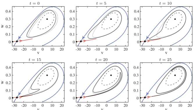
As noted in Sect.1.4, by far the most direct way to detect the presence of shear-induced chaos is to plot the images ofκ(γ )under the unperturbed flow, and to see if folds develop in time. A sample “movie” is shown in Fig.4. As one can see, by
20 10 0 -10 -20 -30 v 0.4 0.3 0.2 0.1 0 w 20 10 0 -10 -20 -30 v 0.4 0.3 0.2 0.1 0 20 10 0 -10 -20 -30 v 0.4 0.3 0.2 0.1 0 20 10 0 -10 -20 -30 v 0.4 0.3 0.2 0.1 0 w 20 10 0 -10 -20 -30 v 0.4 0.3 0.2 0.1 0 20 10 0 -10 -20 -30 v 0.4 0.3 0.2 0.1 0
Fig. 4 Shear-induced folding in the Morris–Lecar model. Here, the stable cycle is given one kick with A= −2, then allowed to relax back to the cycle. The limit cycleγis shown in gray; also shown are the three fixed points (dots), the stable and unstable manifolds of the saddle, and the unstable cycle (dashed
curve)
saddle, while some other points, evidentlyΦt-images of points kicked inside the
unsta-ble cycle, have remained inside, and at t =10 they are beginning to gain on points in the tail in terms of their angular position (or phase) aroundγ. At t = 15, these points have overtaken those in the tail, and the difference is further exaggerated in the last two frames. One would conclude that for the parameters shown, the system very likely has shear-induced chaos.
Because this step can be done quickly for the ML model, we use it to locate param-eters with the desired properties. The kick size used in Fig.4is A = −2, which is quite reasonable physiologically: it takes at least 10–15 kicks of this size to push a neuron over threshold. Figure4also tells us that it takes on the order of 15 units of time for the fold to begin to form, so that for a periodically-kicked system to produce chaos, the kick period should probably be upwards of 20 units of time. (Kicks deliv-ered too frequently may also drive points to the left of the stable manifold of p; once that happens, it will end up near the left sink.)
Figure5shows the strange attractor that results from a periodically-kicked regime.
Lyapunov exponents
Let us now explore the chaotic behavior more systematically. Figure6a shows the largest Lyapunov exponentΛmaxas a function of the kick period T , for a variety of kick amplitudes. More precisely, given a phase point(v0, w0)and a tangent vectorη0, we letη(t)be the solution of the variational equation for the kicked system, and define
Λmax(v0, w0;η0)= lim
t→∞
1
20 10 0 -10 -20 -30 v 0.4 0.3 0.2 0.1 0 -0.1 w
Fig. 5 A strange attractor created by shear-induced chaos. The dashed curves show the basin boundary of the limit cycleγ. Here A= −2,T=27
30 27.5 25 22.5 20 0.02 0 -0.02 -0.04 A=-0.5 30 27.5 25 22.5 20 0.02 0 -0.02 -0.04 A=-1.0 30 27.5 25 22.5 20 0.02 0 -0.02 -0.04 A=-2.0
(a)Lyapunov exponents
Reliable Unreliable 1000 800 600 400 200 Time 20 15 10 5 0 T rial 1000 800 600 400 200 Time
(b)Spike times over repeated trials
Fig. 6 Lyapunov exponents and reliability of the ML system. In a, we plot the Lyapunov exponents. In b, we plot spike times generated by reliable (left) and unreliable (right) systems over repeated trials, with random initial conditions sampled from a neighborhood ofγ. The exponents in a are computed as follows: for each choice of kick amplitude and kick period, six random initial conditions are used to estimate expo-nents via long-time simulations. The max and min are treated as outliers and discarded; the remaining are used to form error bars. The dot marks the median
It is a standard fact that for each(v0, w0), Λmax(v0, w0;η0)is equal to the largest Lyapunov exponent except forη0in a lower dimensional subspace (see, e.g.,
[image:15.439.50.385.286.483.2]For small A, the exponents are predominantly negative, just as we would expect: the dynamical landscape is characterized by sinks and saddles. As A increases, the tendency to form positive exponents becomes greater, so that for A = −2 and suf-ficiently large T , most exponents sampled are positive, confirming the strong form of (sustained and observable) chaos discussed in Sect.1.3. Note, however, that this is only a tendency: the fluctuations seen in the Lyapunov exponents as we vary T are likely real, and reflect the competition between the “horseshoes and sinks” and “strange attractors” scenarios.
As explained in Sect.2, Lyapunov exponents are useful as probes of neuronal reli-ability. This is illustrated in Fig.6b. The left panel there shows the response of a system withΛmax<0: clearly, after some transients, the response of the system is the same across all the trials. In the right panel, we have Λmax > 0, and the resulting spike times show significant variability across trials. Moreover, this variability will persist in time due to the presence of sustained chaos.
We finish with the following two remarks: (1) While we have focused on the periodically kicked case, similar-sized kicks that arrive at random times that are, on average, sufficiently far apart will lead to time-dependent strange attractors for much the same reasons as we have discussed. We will not pursue this here, but refer the reader toLin and Young(2008) andLin et al.(2009a). (2) Notice that the saddle p, which is the root cause of the chaos in the kicked system in the sense that it is responsible for scrambling the order (or phases) of the points on κ(γ ), does not lie that close to the limit cycle. Not only would phase reduction meth-ods miss this effect, but the PRC will offer no hint at all that any breakdown has occurred.
4 Firing rates and interspike intervals
We demonstrate in this section that, as asserted in item (2) of Sect.1.2, “sticky” sets in the boundary of Basin(γ )can lead to discrepancies between the dynamical behavior of the full model and that deduced from the infinitesimal PRC. Specifically, we will present numerical data to show in the example considered that firing rates for the
full model are significantly lower and interspike intervals (ISIs) are longer and more spread out than those predicted by the PRC.
For the unperturbed flow, we continue to use the example from the last section, with the same parameters. Recall that this system is in the “homoclinic regime” of ML, with a limit cycle we call γ. Shown in dashed lines in Fig. 5 are part of
1 0.8 0.6 0.4 0.2 0 0.06 0.05 0.04
Firin
g
rate
Forcingamplitude
0.03 0.02 0.01 0
20 10 0 -10 -20 -30
v
0.4 0.3 0.2 0.1 0 -0.1
w
[image:17.439.77.365.54.195.2](a) (b)
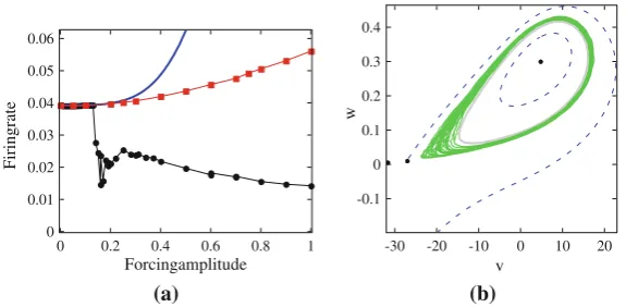
Fig. 7 Firing rate statistics of the stochastically-forced ML model. In a, we compare of firing rates for the full ML system and its phase reduction driven by white noise. Black dots full ML. Red squares empirical phase reduction firing rate. Solid blue curve: Perturbative formula for PRC firing rate (see Eq. (5)). b shows a long sample path forβ=0.2 (color figure online)
Instead of periodic forcing, here we drive the oscillator with white noise in addition to the steady current I0, i.e., we let I(t)=I0+β·Cm· ˙W ,6and consider the random dynamical system that results from looking at one realization ofW at a time. For the˙
phase reduced model, it is natural to regard the system as producing one spike as it passes through a marked point on the cycle. For the full ML model, it is necessary to fix an artificial definition of what it means for the system to “spike”: we define a reset to be when the voltage falls below−10, and say the neuron “spikes” when (after a reset) the voltage rises above +12.5. See Fig.5for how this corresponds to the location of the limit cycle.
Comparison of firing rates The results are shown in Fig.7a. Plotted are firing rates as a function of the drive amplitudeβfor three different systems: (i) the full ML system; (ii) the firing rate of the phase reduction, computed empirically; and (iii) the firing rate of the phase reduction as computed by the perturbative formula (5) of Ly and Ermentrout. We plot both (ii) and (iii) because Eq. (5) is itself an approximate result based on the phase reduction (4), valid only for smallβ. As one would expect, for smaller forcing amplitudes (<0.1), all three agree. Asβ increases, the perturbative formula tracks the empirical firing rate of the phase reduction fairly well, but neither of these PRC-based predictions capture the dramatic drop in firing rate of the full system occurring aroundβ = 0.2. Simulations (an example of which is shown in Fig.7b) show that the precipitous drop in firing rate in this case has to do with trajectories spending more time near the saddle p.
Comparison of ISI distributions Figure8shows the numerically computed ISI distri-butions for the full ML model and for the phase reduction (4).7For small noise, we see
6 The constant Cmis the membrane capacitance. With this scaling,βhas the dimension voltage/√time ;
this makes its magnitude relative to the membrane voltage easier to assess.
7 We note thatLy and Ermentrout(2011) also contains an explicit small-βexpansion of the ISI distribution.
100 80 60 40 20
Interspiketimeinterval 0.1
0.075
0.05
0.025
0
amp=0.25
100 80 60 40 20 0.08
P
robab
.density
0.06
0.04
0.02
0
amp=0.5
100 80 60 40 20 0.06
0.04
0.02
0
amp=1.0
[image:18.439.81.363.56.295.2]Interspiketimeinterval Interspiketimeinterval
Fig. 8 interspike interval (ISI) distributions for variousβ. Solid black lines ISI histograms for the full ML system. Dashed blue lines ISI histograms for the phase reduction (4) (color figure online)
the full ML system and phase reduction agree fairly well: the ISI distribution is concen-trated around the period of the cycle (about 25.2), and the shape is roughly gaussian. As noise amplitude increases, we see in the full ML system (i) a broadening of the ISI distribution, and (ii) an overall shift toward larger ISIs. Neither of these effects are captured by the PRC, as they involve structures a finite distance away fromγ.
Finally, to compare the tails of the ISI distributions, here are the fraction of ISIs greater than 2×(cycle period):
β Full ML PRC
0.25 0.0225 0.0003 0.5 0.127 0.0032 1.0 0.322 0.0013
Notice that the PRC systematically under-predicts the probability of a long interspike interval, consistent with the “trapping” effect of nearby invariant structures.
5 Altered spiking patterns in bistable systems
Fig. 9 ML phase portrait in the Hopf regime. Shown are a limit cycle surrounding an unstable cycle, which in turn surrounds a sink. Here, I0=90,
corresponding to an unforced period of about 102 ms
20 0
-20 -40
v
0.5
0.4
0.3
0.2
w
Full ML,
10000 8000
6000 4000
2000 0
40 20 0 -20 -40 -60
v(t)
Full ML,
10000 8000
6000 4000
2000 0
40 20 0 -20 -40 -60
v(t)
PRC,
10000 8000
6000 4000
2000 0
40 20 0 -20 -40 -60
v(t)
Fig. 10 Voltage traces for the ML system in Hopf regime. The top two panels show simulation using the full ML model with the indicated level of stochastic forcing. The bottom panel shows the PRC using
β=0.4. Here, I0=90
For the unperturbed system, we consider here parameters of ML that put it in a “Hopf regime”, with I0≈90. Precise parameters used are given in the Appendix, and some relevant dynamical structures are shown in Fig.9. In this regime, the system has a limit cycle, which we callγ. Each time an orbit passes near the right-most point ofγ, we think of it as producing a “spike”. Notice that this system is bistable: insideγthere is a sink, the basin of attraction of which is separated from the basin ofγby a repelling periodic orbit (from a Hopf bifurcation). This repelling periodic orbit is very close to
We now consider perturbations to the ML model above. As in Sect.4, we again use a white-noise perturbation, i.e., I(t)=I0+β·Cm· ˙W.Figure10shows the resulting
voltage traces of the full model and PRC predictions (computed at I0=90). The top panel shows the full ML simulation withβ=0.2 (a relatively weak forcing), starting the trajectory onγ. Since the basin of the sink, i.e., the unstable periodic orbit shown in Fig.9, is so close to the limit cycleγ, a trajectory followingγcan easily get pushed into the basin, and then attracted to the sink. This can happen even with very smallβ. The sink itself, however, is a little farther from the boundary of its basin, so it is more difficult for a trajectory near the sink to escape under weakβ. This is why for weak noise likeβ=0.2, it is easy to observe a transition fromγto the sink, but not easy to see transition in the reverse direction.
Forβa little larger, e.g.,β =0.4, the trajectory jumps back and forth more readily: it alternately follows (roughly) the limit cycleγ and stays near the sink, switching between the “spiking” and “quiescent” modes at somewhat random times. Not surpris-ingly, in the phase-reduced model (bottom panel), these perturbations do not have a significant impact, and the spiking ranges from completely regular to slightly irregular in the second case due to the effect of the noise. PRC voltage traces forβ =0.2 (not shown) are quite similar.
Finally, we note that in this bistable situation, a neuron can exhibit substantial sub-threshold activity. The PRC underestimates the extent of such activity.
6 Conclusions
This paper compares two ways of evaluating an oscillator’s response to perturbations: phase reductions versus analysis of the full model. We have found that the infinites-imal PRC, which has the virtue of being straightforward to construct and reducing model dimensionality, produces regular oscillatory behavior even when the full model does not. Specifically, we presented examples from the Morris–Lecar neuron model to show that
(i) Periodic kicking of the ML system can lead to unreliable response in the full model via the mechanism of shear-induced chaos, contrary to PRC predictions. (ii) When stochastically driven, stickiness of nearby invariant structures can lead
to lower firing rates and longer ISIs compared to PRC predictions.
(iii) The forcing need not be strong to bring about serious discrepancies in firing patterns between full and phase-reduced models.
Moreover, in all the situations examined, the phase reduction itself offers no hint that any breakdown has occurred.
While we have focused on the ML model for illustration, the geometric ideas we used are quite general, and we expect similar phenomena to occur in a variety of settings that involve rhythms and oscillations.
Finally, given that pure phase reductions cannot always capture the behavior of high dimensional nonlinear oscillators, are there alternative methods that give better characterizations? One classical technique, which has seen relatively little applica-tion in biological modeling, is that of moving-frame coordinates for the analysis of periodic orbits. This is nicely described inHale(1969) and recently advocated in a neuroscience context byMedvedev(2011), and for electronic circuits in ¸Suvak and Demir(2011). In essence this offers a coordinate transformation to a phase–amplitude system that allows one to track the evolution of distance from the cycle as well as phase on the cycle. We are currently developing this approach and using it to better understand the three points listed above. This, and a framework for understanding the dynamics of weakly coupled phase–amplitude models, will be presented elsewhere.
Acknowledgments We thank one of the anonymous referees for pointing out¸Suvak and Demir(2011). KKL is supported in part by the US National Science Foundation (NSF) through grant DMS-0907927. KCAW and SC acknowledge support from the CMMB/MBI partnership for multiscale mathematical mod-elling in systems biology-United States Partnering Award; BB/G530484/1 Biotechnology and Biological Sciences Research Council (BBSRC). LSY is supported in part by NSF grant DMS-1101594.
Open Access This article is distributed under the terms of the Creative Commons Attribution License which permits any use, distribution, and reproduction in any medium, provided the original author(s) and the source are credited.
Appendix: Morris–Lecar model details
Here we briefly summarize the details of the ML model used in this paper. The inter-ested reader is referred toErmentrout and Rinzel(1991) andErmentrout and Terman
(2010) for more details. Recall the ML equations
Cm v˙=I(t)−gleak·(v−vleak)−gKw·(v−vK)−gCam∞(v)·(v−vCa)
˙
w=φ·(w∞(v)−w)/τw(v).
As explained in Sect.2, the ML model tracks the membrane voltagev and a gating variablew. The constant Cm is the membrane capacitance,φa timescale parameter,
and I(t)an injected current.
Spike generation depends crucially on the presence of voltage-sensitive ion chan-nels that are permeable only to specific types of ions. The ML equations include just two ionic currents, here denoted calcium and potassium. The voltage response of ion channels is governed by thew-equation and the auxiliary functionsw∞,τw, and m∞, which have the form
m∞(v)= 1
2[1+tanh((v−v1)/v2)],
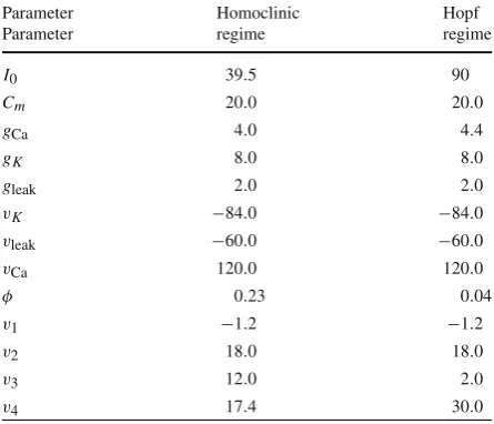
Table 1 ML parameter values
used in this paper Parameter Homoclinic Hopf
Parameter regime regime
I0 39.5 90
Cm 20.0 20.0
gCa 4.0 4.4
gK 8.0 8.0
gleak 2.0 2.0
vK −84.0 −84.0
vleak −60.0 −60.0
vCa 120.0 120.0
φ 0.23 0.04
v1 −1.2 −1.2
v2 18.0 18.0
v3 12.0 2.0
v4 17.4 30.0
w∞(v)= 1
2[1+tanh((v−v3)/v4)].
The function m∞(v)models the action of the relatively fast calcium ion channels;vCa is the “reversal” (bias) potential for the calcium current and gCathe corresponding conductance. The gating variablewand the functionsτw(v)andw∞(v)model the dynamics of slower-acting potassium channels, with its own reversal potentialvKand conductance gK. The constantsvleakand gleakcharacterize the “leakage” current that is present even when the neuron is in a “quiescent” state. The forms of m∞,τw, and
w∞(as well as the values of thevi) can be obtained by fitting data, or reduction from
more biophysically-faithful models of Hodgkin-Huxley type (see, e.g.,Ermentrout and Terman 2010).
The precise parameter values used in this paper are summarized in Table1. These are obtained fromErmentrout and Terman(2010).
References
Afraimovich VS, Shilnikov LP (1977) The ring principle in problems of interaction between two self-oscil-lating systems. J Appl Math Mech 41:618–627
Brown E, Moehlis J, Holmes P (2004) On the phase reduction and response dynamics of neural oscillator populations. Neural Computat 16:673–715
Cohen AH, Rossignol S, Grillner S (eds) (1988) Neural Control of rhythmic movements in vertebrates. Wiley, New York
Dayan P, Abbott L (2001) Theoretical neuroscience: computational and mathematical modeling of neural systems. MIT Press, Cambridge
Deville REL, Sri Namachchivaya N, Rapti Z (2011) Stability of a stochastic two-dimensional non-Hamil-tonian system. SIAM J Appl Math 71:1458–1476
Eckmann J-P, Ruelle D (1985) Ergodic theory of chaos and strange attractors. Rev Mod Phys 57:617–656 Ermentrout GB, Kopell N (1991) Multiple pulse interactions and averaging in coupled neural oscillators.
Ermentrout GB, Rinzel J (1991) Analysis of neural excitability and oscillations. In: Koch C, Segev I (eds) Methods in neuronal modeling: from synapses to networks. Bradford Books, Bradford
Ermentrout GB, Terman DH (2010) Mathematical Foundations of Neuroscience. In: Interdisciplinary applied mathematics, vol 35. Springer, Berlin
Glass L, Guevara MR, Belair J, Shrier A (1984) Global bifurcations of a periodically forced biological oscillator. Phys. Rev. A 29:1348–1357
Glass L, Mackey MC (1988) From clocks to chaos: the rhythms of life. Princeton University Press, New Jersey
Golubitsky M, Stewart I, Buono PL, Collins JJ (1999) Symmetry in locomotor central pattern generators and animal gaits. Nature 401:693–695
Guckenheimer J (1974) Isochrons and phaseless sets. J Theor Biol 1:259–273
Guckenheimer J, Holmes P (1983) Nonlinear oscillations, dynamical systems, and bifurcations of vector fields. Springer, Berlin
Hale JK (1969) Ordinary Differential Equations. Wiley, New York
Hoppensteadt FC, Izhikevich EM (1997) Weakly connected neural networks. Springer, Berlin
Lin KK (2006) Entrainment and chaos in a pulse-driven Hodgkin–Huxley oscillator. SIAM J Appl Dyn Sys 5:179–204
Lin KK, Young L-S (2008) Shear-induced chaos. Nonlinearity 21:899–922
Lin KK, Young L-S (2010) Dynamics of periodically-kicked oscillators. J Fixed Point Theory Appl 7:291– 312
Lin KK, Shea-Brown E, Young L-S (2009) Reliability of coupled oscillators. J Nonlinear Sci 19:630–657 Lin KK, Shea-Brown E, Young L-S (2009) Reliability of layered neural oscillator networks. Commun Math
Sci 7:239–247
Lin KK, Shea-Brown E, Young L-S (2009) Spike-time reliability of layered neural oscillator networks. J Comput Neurosci 27:135–160
Lu K, Wang Q, Young L-S (2012) Strange attractors for periodically forced parabolic equations. Mem Am Math Soc (to appear)
Ly C, Ermentrout GB (2011) Analytic approximations of statistical quantities and response of noisy oscil-lators. Physica D 240:719–731
May RM (1972) Limit cycles in predator–prey communities. Science 177:900–902 Medvedev GS (2011) Synchronization of coupled limit cycles. J Nonlinear Sci 21:441–464
Mirollo RE, Strogatz SH (1990) Synchronization of pulse-coupled biological oscillators. SIAM J Appl Math 50:1645–1662
Netoff TI, Acker CD, Bettencourt JC, White JA (2005) Beyond two-cell networks: experimental measure-ment of neuronal responses to multiple synaptic inputs. J Comput Neurosci 18:287–295
Oprisan SA, Thirumalai V, Canavier CC (2003) Dynamics from a time series: can we extract the phase resetting curve from a time series? Biophys J 84:2919–2928
Ott W, Stenlund M (2010) From limit cycles to strange attractors. Commun Math Phys 296:215–249 Pikovsky A, Rosenblum M, Kurths J (2001) Synchronization: a universal concept in nonlinear sciences.
Cambridge University Press, Cambridge
¸Suvak Ö, Demir A (2011) On phase models for oscillators. IEEE Trans Comput Aided Des Integrated Circ Syst 30:972–985
Thul R, Bellamy TC, Roderick HL, Bootman MD, Coombes S (2008) Calcium oscillations. In: Maroto M, Monk N (eds) Cellular oscillatory mechanisms, advances in experimental medicine and biology. Springer, Berlin
Wang Q, Ott W (2011) Dissipative homoclinic loops of two-dimensional maps and strange attractors with one direction of instability. Commun Pure Appl Math 64:1439–1496
Wang Q, Young L-S (2001) Strange attractors with one direction of instability. Commun Math Phys 218:1–97
Wang Q, Young L-S (2002) From invariant curves to strange attractors. Commun Math Phys 225:275–304 Wang Q, Young L-S (2003) Strange attractors in periodically-kicked limit cycles and Hopf bifurcations.
Commun Math Phys 240:509–529
Wang Q, Young L-S (2008) Toward a theory of rank one attractors. Ann Math 167:349–480 Winfree A (2000) Geometry of biological time, 2nd edn. Springer, Berlin
Young L-S (2002) What are SRB measures, and which dynamical systems have them? J Stat Phys 108:733– 754