A&A 573, A112 (2015)
DOI:10.1051/0004-6361/201322250 c
ESO 2015
Astronomy
&
Astrophysics
Photoionising feedback and the star formation rates in galaxies
J. M. MacLachlan
1, I. A. Bonnell
1, K. Wood
1, and J. E. Dale
21 SUPA, School of Physics & Astronomy, University of St. Andrews, North Haugh, St. Andrews KY16 9SS, UK e-mail:iab1@st-andrews.ac.uk
2 Excellence Cluster “Universe”, Boltzmannstr. 2, 85748 Garching, Germany
Received 10 July 2013/Accepted 11 October 2014
ABSTRACT
Aims.We investigate the effects of ionising photons on accretion and stellar mass growth in a young star forming region, using a
Monte Carlo radiation transfer code coupled to a smoothed particle hydrodynamics (SPH) simulation.
Methods.We introduce the framework with which we correct stellar cluster masses for the effects of photoionising (PI) feedback and
compare to the results of a full ionisation hydrodynamics code.
Results.We present results of our simulations of star formation in the spiral arm of a disk galaxy, including the effects of photoionising
radiation from high mass stars. We find that PI feedback reduces the total mass accreted onto stellar clusters by≈23% over the course of the simulation and reduces the number of high mass clusters, as well as the maximum mass attained by a stellar cluster. Mean star formation rates (SFRs) drop fromSFRcontrol=4.2×10⁻²Myr−1toSFRMCPI=3.2×10⁻²Myr−1after the inclusion of PI feedback
with a final instantaneous SFR reduction of 62%. The overall cluster mass distribution appears to be affected little by PI feedback.
Conclusions.We compare our results to the observed extra-galactic Schmidt-Kennicutt relation and the observed properties of local
star forming regions in the Milky Way and find that internal photoionising (PI) feedback is unlikely to reduce SFRs by more than a factor of≈2 and thus may play only a minor role in regulating star formation.
Key words.HII regions – radiative transfer – stars: massive
1. Introduction
Feedback from young massive stars can have a significant im-pact on their environment on scales of tens of au to several kpc (Hollenbach et al. 2000;Franco et al. 1994;Tenorio-Tagle 1979; Whitworth 1979), and is often invoked to regulate star forma-tion rates (SFRs) in galaxies. The emission of high frequency photoionising photons into the surrounding neutral gas can act to unbind the gas and disrupt ongoing star formation. On small scales the action of PI photons from the central star is a principal mechanism for the dispersal of circumstellar disks around mas-sive stars (Hollenbach et al. 2000;Bally et al. 1998). In dense cluster environments the photoevaporation by an external source can cause the destruction of circumstellar disks, even around low mass stars, if the cluster is large enough to host an O or B star.
It is thought that a large fraction of stars form in clusters em-bedded within molecular clouds rather than in isolation (Lada et al. 1991; Lada & Lada 2003) and so the action of massive stars can strongly affect the growth and evolution of other cluster members. In the case where ionised gas becomes unbound and escapes from the cluster, then it can lead to the complete dis-ruption of the stellar cluster (Hills 1980;Baumgardt & Kroupa 2007;Goodwin & Bastian 2006).
In addition to limiting the ability of stars to accrete neutral gas, the influence of ionised gas can also promote the forma-tion of new stars. This may be due to the “collect and collapse” mechanism in which neutral gas is swept up by the advancing ionisation front and forms unstable clumps that undergo collapse and form stars (Whitworth et al. 1994;Elmegreen & Lada 1977; Dale et al. 2007a). Alternatively additional star formation may be caused by the radiatively driven implosion of pre-existing stable gas clumps that exist in the structure of the undisturbed
molecular cloud (Kessel-Deynet & Burkert 2003;Bisbas et al. 2011).
It has been shown by previous authors (Dale et al. 2005;Dale & Bonnell 2011;Krumholz et al. 2005) that the underlying struc-ture of the neutral gas in which an ionising source is embedded will have a strong influence on the propagation of ionising pho-tons. If the source is accreting from high density accretion flows, then these will strongly inhibit the flow of PI photons in cer-tain directions and effectively shield portions of the surround-ing medium from the direct effects of the source. The ionising photons will escape more easily into the low density cavities of the surrounding gas, and the accretion flows can remain mostly neutral.
Smoothed particle hydrodynamics (SPH) provides a use-ful method to follow the evolution of a molecular cloud where large contrasts in gas densities are present. The Lagrangian na-ture of SPH codes also helps in following the evolution of self-gravitating flows, but traditional methods for evaluating the transfer of radiation in such environments are often best suited to Eulerian schemes, where the optical depth can be more simply integrated along directions of photon travel. Several authors have implemented radiation transfer methods in SPH simulations to treat PI radiation (Dale et al. 2005,2007b;Gritschneder et al. 2009;Kessel-Deynet & Burkert 2000). While methods exist to implement radiation transfer in SPH codes, many simulations still neglect such effects for the sake of computational speed and complexity.
We have used a Monte Carlo photoionisation (MCPI) code to calculate the ionisation structure for a series of static, inde-pendent snapshots of the SPH simulation. We do not re-run the SPH simulation but instead use the MCPI code to estimate which of the SPH particles become photoionised by young stars and remove their contribution to future star formation. There is no
additional computational overhead during the SPH simulation as all photoionisation calculations are performed once the sim-ulation is completed. In this way we are able to characterise the reduction in SFRs and efficiency caused directly by PI feedback. The aim of this work is to provide an estimate of the first order effects of feedback from PI radiation. We first test our method against a full ionisation hydrodynamic simulation before apply-ing it to star formation in a galactic spiral arm.
2. SPH simulations
We begin our investigation with the star formation simulations ofBonnell et al.(2013). These are designed to track the small scale star formation processes as well as the large scale evolution of the interstellar medium on galactic scales. Three simulations were carried out byBonnell et al.(2013). Firstly a global disk simulation of a 5−10 kpc annulus of material within a galac-tic disk was evolved for 370 Myr. Cooling in the spiral shocks produced a complex, multiphase interstellar medium in which dense clouds reminiscent of the molecular clouds seen within our own galaxy formed. To follow the star formation process within such dense clouds a second high resolution run was then carried out, theCloudsimulation. This followed the formation of one dense cloud at higher resolution than the initial global simulation. Finally, theGravitysimulation added the effects of self-gravity and allowed the dense cloud to form stars from the realistic initial conditions provided by theCloudsimulation. The Gravitysimulation contains 1.29×10⁷SPH particles with each particle having a mass of 0.15M. The formation of stars was treated with the use of sink particles (Bate et al. 1995). Due to the prescription of the formation of a sink particle which re-quires a minimum of 70 particles we are only able to resolve the gravitational collapse to a mass of≈11M. This is too high to represent low mass star formation and each sink should in-stead be thought of as a stellar cluster. The results fromBonnell et al.(2013) based on theGravitysimulation suggest that the observed Schmnidt-Kennicutt (Schmidt 1963;Kennicutt 1998) power law relation between star formation rate and gas surface density can be explained by the combination of spiral shocks and gas cooling rates. However, the star formation rates produced by the simulation are higher than those observed.
We start our investigation with theGravitysimulation. The dense cloud it represents is approximately 250 pc in size and contains≈1.7×10⁶ M of gas. We assume that no prior star formation has occurred in the cloud or its surroundings during its previous evolution. The star formation and evolution of the cloud is traced for∼5 Myr. Beyond this point it is likely that su-pernovae within the cloud will quickly act to disperse it, ending most star formation. We assume that all gas forming or accret-ing onto a sink particle is retained by the sink and that none is recycled back into the simulation by feedback on the scale of the small clusters represented by the sinks. Star formation effi cien-cies are unlikely to be this high and evidence suggests that they are in the region 25−50% (Olmi & Testi 2002) which would lead to our star formation rates being upper limits by a factor 2−4.
During the time evolution of theGravitysimulation the prop-erties of each SPH particle (position, velocity etc.) are printed out to file at several points. It is on these outputs that we base our analysis regarding the effects of photoionisation on the star formation process.
3. Monte Carlo photoionisation code
In order to calculate the photoionisation of the gas throughout the star forming region during its evolution we use a MCPI code
x (kpc)
z (kpc)
−0.1 −0.05 0 0.05 0.1
−0.1 −0.05 0 0.05
0.1 Sinks
[image:2.595.322.544.73.296.2]Ionization sources
Fig. 1. Positions of the stellar sink particles (black circles) and the ionising sources at the end of the SPH simulation (356 Myr) with
Σgas=4Mpc−2.
described inWood & Loeb(2000) and extended byWood et al. (2010). The routines can be used to calculate the hydrogen-only photoionisation and have been modified to allow the use of SPH data as initial input. The Monte Carlo treatment of the radiation transfer is fully 3D and can easily treat the complex geometries encountered within the gas distribution.
All ionising photons encounter an average opacity which is given bynH0σ¯+nHσdust, wherenH0is the number density of neu-tral hydrogen, ¯σis the flux averaged cross section andσdustgives
the dust cross section per hydrogen atom (i.e. cm−2 H−1). Two
different flux averaged cross sections are considered depending on whether a photon has been emitted directly by an ionising source (direct photon) or is the product of absorption and sub-sequent reemission (diffuse photon). The cross section for direct photons is averaged over the flux
¯
σ=
∞
ν0Fσνdν
Fdν , (1)
where F is the source ionising spectrum, ν0 is the frequency
of the Lyman edge andσ is the absorption cross-section for Hydrogen. In the case of the diffuse ionising spectrum the pho-ton energies are strongly peaked at just above 13.6 eV and so we set the cross section for the diffuse photons to the hydrogen cross-section just above 13.6 eV, ¯σ = 6.2×10⁻¹⁸ cm−2. This
simplification means that essentially only two frequencies are considered and greatly speeds the computation of the ionisation fractions throughout the grid.
As an output of the photoionisation code we have a grid con-taining the neutral fraction (fn) which gives the fraction of the
mass in each grid cell which is neutral, with the remainder being ionised. In order to apply our MCPI routines to the SPH data it is necessary to discretise the SPH density estimate across a carte-sian grid. In this case each SPH simulation dump is discretised onto a 2003grid of cells. For theGravitysimulation we centre
a 1 pc resolution for the MCPI simulations. We found that an in-creased resolution (a 23increase in grid cells) has little impact on
the results (of order a 1 per cent change in the ionised gas mass) of the MCPI code, but adds significantly to the time required for each simulation.
3.1. Ionising photon numbers
To estimate the positions and locations of ionising sources within the molecular cloud we create a list of all stellar sink particles in the simulation along with their locations. Due to the limited mass resolution of the simulations each sink particle represents a stellar cluster in this case. The number of photons able to ionise hydrogen produced each second by each stellar cluster is repre-sented by theQHvalue. Following the method ofDale & Bonnell
(2011) we assign aQHto clusters that exceed 600 Mby
cal-culating the total mass in stars M > 30 M and dividing this mass by 30M. This gives an approximate measure of the num-ber of 30 M stars, N30. To estimate QH for a 30 M O-star
we fit the data ofConti et al.(2008; Table 3.1) andDiaz-Miller et al.(1998; Table 1) to find a relation between the stellar mass and number of ionising photons. From this we estimate that the number of ionising photons produced by a 30Mstar will be QH=2.8×1048s−1.
We assume a Salpeter IMF with upper and lower mass limits of 100Mand 0.1 M. The use of a Salpeter IMF slope down to 0.1Mis an overestimate of the total mass in low mass stars as the true IMF should turn over near 0.5 M (Kroupa et al. 1993). This will lead to lead to under-estimates for the mass in stars>30 M, but is likely offset by our assumption of as 100 per cent star formation efficiency. We performed a test simu-lation using a two-part Kroupa IMF (Kroupa 2001) and included mean values ofQHfrom stochastic sampling. The ionising fluxes
in this case was typically a factor of 2 higher than given by our regular estimate, but this increase is less than that due to our assumed 100 per cent star formation efficiency, which likely overestimates the total stellar mass by a factor 2−4. Dale et al. (2012a) find that uncertainties in the ionising fluxes of factors of a few have little impact in the ionised gas mass. We can reason-ably conclude that these simulations are likely to encompass the maximum impact of photoionising feedback. It is possible that the stochastic sampling of the IMF could result in significantly larger fluxes at low cluster masses in rare cases with a high-mass star in isolation or in a low-mass cluster. We do not consider such cases here.
4. Coupling the MCPI to SPH simulations
As the time evolution of the SPH simulation we are investigating has previously been completed and did not include the effects of photoionisation, it is necessary to approximate the feedback ef-fects as well as possible without rerunning the simulation itself. By linking our MCPI codes to the individual time dumps of the SPH code we hope to investigate the effects that photoionisation by young stars can have on the mass accretion rates during the course of the simulation. To accomplish this we have included a series of checks on each SPH gas particle, that are carried out at each SPH time dump in the simulation.
We initially begin at the point in the simulation where at least one stellar sink has a mass≥600M, as this will provide the first source of ionising photons as described in Sect.3. We then run our MCPI code using as inputs the SPH density discretised into a cartesian grid and the positions andQHvalues for the stellar
clusters. The output of the the MCPI code is a grid containing the
hydrogen ionisation fraction throughout the star forming region at the time-step of interest.
Once the MCPI code has computed the ionisation fraction within the grid we identify the SPH particles that are located within ionised cells. If a gas phase SPH particle is located in a cell with an neutral fraction (fn) < 0.5 then it is classified as
an ionised particle. We have found that in general the results we obtain are relatively insensitive to the exact value of fn at
which particles are classed as ionised, as the mass of ionised par-ticles is dominated by SPH parpar-ticles that are almost fully ionised (fn<0.1).
We adjust the accretion rates by removing any mass accreted from an “ionised” SPH particle as such gas should no longer be gravitationally bound to the accreting sink. The stellar cluster masses are recalculated by removing an amount of mass from the sink equal to the mass of the ionised particle multiplied by (1−fn). In this way if an accreted ionised particle was found in a
cell with fn=0.4 then 60% of its mass would be prevented from
accreting onto the stellar sink. ionised gas is assumed to escape the simulation and be no longer available for star formation. This means that the ionisation fraction cannot decrease. In testing this approach, we found that few particles ever returned to a neutral status as once they are exposed to the ionising radiation, they did not re-enter a shadowed region in these simulations. We also test for the ionisation of the SPH particles that are used to ini-tially form stellar sinks. If, when a sink particle is formed, more that 50% of the gas particles that took part in its formation were classified as ionised, then the sink will be removed from further calculations and assumed not to form.
This method allows us to investigate the effects of ionisation feedback on the accretion onto stellar clusters as the simulation progresses and compare the results with the initial distributions that do not include any effects of photoionisation by massive stars.
It is important to note that no dynamical effects of the pho-toionisation are included. Thus the pressure from the hot gas onto the surrounding environment is ignored as is the reduc-tion of gravitareduc-tional accelerareduc-tion from the reduced sink masses in the simulation. The gravitational and pressure forces which were used to determine the dynamics are entirely due to the non-ionising runs with higher sink masses and fully neutral gas. This is an unfortunate but unavoidable effect of our approach and therefore we have first compared this approach to the full dynamical ionisation simulations from Dale et al. (2012). The fact that we are able to largely replicate the Dale results (see be-low) has allowed us to proceed with this approach with a high level of confidence in the results.
5. Validity of the method
Table 1.Properties of the simulations from D12 used to test the MCPI method.
Run Mass Radius vrms n(H2) tff T (M) (pc) (kms−1) (cm−3) (Myr) (K)
A 106 180 5.0 2.9 19.6 143
I 104 10 2.1 136 2.56 53
In run I the mass resolution is sufficient to consider the sink parti-cles that form as individual stars and so we can directly estimate number of ionising photons produced from the stellar mass. We adopt the same method as D12 to calculate theQHvalues in run I
and assign any sink that exceeds 20M a number of ionising photons according to the relation:
log(QH)=48.1+0.02(M−20M), (2)
whereM is the stellar mass. In run A we adopt the standard relation between cluster mass and number of ionising photons from Sect.3.1.
For both run A and I we have access to the control simu-lations, which included no ionisation effects (hereby referred to as the control runs), and also the simulations including the ef-fects of ionisation. We apply our methods to the control runs and compare the results to the simulations which explicitly in-cluded ionisation. In this way, we can assess how important the dynamics of the ionised gas are, which we cannot follow in our MCPI method.
For run A we have an excellent agreement between our cal-culations and D12 over most of the time covered by the simula-tion. The integrated SFR, calculated from the total stellar mass formed during the simulation isSFRcontrol=3.6×10⁻³Myr−1
in the control and drops toSFRDale = 2.8×10⁻³ Myr−1 and SFRMCPI=2.5×10⁻³Myr−1in the D12 and MCPI simulation
respectively.
For run I the integrated SFR for the control isSFRcontrol =
1.1×10⁻⁴M
yr−1and drops toSFRDale=7.1×10⁻⁵ Myr−1
for the D12 simulation andSFRMCPI=5.7×10⁻⁵Myr−1in the
MCPI run.
5.1. Cumulative stellar mass
In Figs. 2 and 3 we present the cumulative stellar sink mass formed over the course of the run A and run I simulations in the control, D12 and MCPI implementations. In run A we have a good agreement between the two methods at most times and the difference in the stellar mass is less than 5% for the majority of the simulation, with the exception of the final few timesteps where the SFR in D12 increases significantly with a correspond-ing change in the stellar mass.
The results from run I are also in reasonable agreement. The MCPI tends to overestimate the effects of feedback at all times with a steady divergence of the stellar sink masses over the course of the simulation. By the end of the run the diff er-ence is around 20%. Again the difficulties of the MCPI method in correctly treating run I are not unexpected due to the strong dynamical influence of the ionised gas.
The fact that the MCPI results are in reasonable agreement with the more sophisticated D12 treatment gives us encourage-ment that we are able to treat the ionisation feedback on stellar growth in a satisfactory way. It should also be noted that mostly the MCPI method predicts a SFR that is equal to or lower than D12. The MCPI treatment can then be interpreted as providing
0.5x10⁴ 1.0x10⁴
1.5x10⁴ 2.0x10⁴ 2.5x10⁴
3.0x10⁴
3.5x10⁴ 4.0x10⁴
8 10 12 14 16 18 20 22 24
Stellar Mass (M
sun
)
Time (Myrs) Control
Dale MCPI
Fig. 2.Cumulative stellar sink mass formed during run A for the control (black), Dale photoionisation (green) and MCPI (blue) runs.
2.0x10²
4.0x10²
6.0x10²
8.0x10² 1.0x10³ 1.2x10³ 1.4x10³
Stellar Mass (M
sun
)
Time (Myrs)
2 4 6
[image:4.595.46.283.109.159.2]Control Dale MCPI
Fig. 3.Same as Fig.2but for run I.
an upper limit to the effects of ionising feedback by only allow-ing it to reduce the SFRs and not accountallow-ing for the possible triggering of star formation.
6. Results
In Fig. 4 we plot the time evolution of the ionised gas mass and ionising luminosity as calculated by the MCPI simulation at each timestep from our SPH simulation. The total ionis-ing luminosity grows steadily throughout the simulation from 0.29−6.6 ×1049 s−1 as the sink particles accrete more mas.
[image:4.595.323.539.294.474.2]Time (Myrs)
Ioniz
ed Gas Mass (M
solar
)
353 354 355 356
104
1 2 3 4 5 6
Ionizing Luminosity (10
49
s
−
1)
Ionized Gas Mass Ionizing Luminosity
Fig. 4.Evolution of the ionised gas-mass and ionising luminosity are plotted as a function of time from the MCPI simulation. The ionised gas mass shown here does not include any gas that has been ionised previously, but was accreted in our control run at the same point in time. Thus the total ionised mass implied by our MCPI simulations is the sum of the ionised gas present at each timestep (shown here) and that subtracted from the stellar mass due to being ionised (Fig.7).
accreted in our control runs, and therefore not present to be ionised. Thus, the total amount of ionised gas implied in our simulations is not just the gas ionised at each time step (Fig.4), but also includes any accreted gas that was previously ionised and therefore subtracted from the total stellar mass as shown in Fig.7.
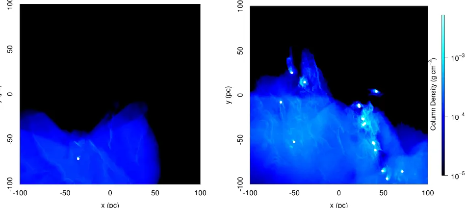
Figure6shows the distribution of the ionised gas particles at the first time step containing an ionising source (left panel) and at the end of theGravitysimulation. Figure5shows the neutral gas surface density at the corresponding times. It can be seen that even in the early stages of PI feedback the ionising photons are able to affect a large region of the cloud. However, much of the gas which has been ionised at large distances from the ionising sources is low density, diffuse gas, that is not currently actively star forming. By the end of theGravitysimulation the ionised gas has filled a large region of the cloud, with highly ionised regions within the dense inner core of the cloud close to the most massive ionising sources. The region of the cloud in the upper section of the plot (y >0) is largely unaffected by the PI photons. This is due to a reduced star formation rate in this region and in the shielding from the high density gas in the central region of the cloud, preventing the propagation of ionising photons in this direction. This has the effect that the low-level of star formation in the upper region (y >0) is largely unaffected by PI feedback from the massive clusters near the cloud centre.
In Fig.7we show the cumulative mass which has been ac-creted onto the stellar sink particles as a function of time from the point at which the first ionising source forms until the end of the simulation. It can be seen that there is a steady divergence of the standard and photoionised cases due to the ionisation of gas particles, any accretion of which is discounted in our pho-toionisation models. We stress that this is simply a reduction in the estimate of the mass in sinks and the corresponding star for-mation rates. The actual dynamics are unaffected as they were calculated in our control, non-ionising SPH simulation. We find that, in total, after our inclusion of photoionisation effects the fi-nal mass accreted by all sinks falls fromMcontrol=2.2×10⁵M
toMMCPI=1.7×10⁵Mwhich is a reduction in the stellar mass
of≈23%.
We estimate the mean SFR over the course of the simulation for both runs by taking the total mass formed by the end of the simulation and dividing by the total time for theGravity simula-tion. In the control run we achieveSFRcontrol =0.042Myr−1, while in the case including photoionisation the rate drops to SFRMCPI=0.032Myr−1. This change is due to feedback from
ionising sources which have previously formed, ionising gas be-fore it can be accreted onto stellar sinks or from new sinks.
The effect of the PI feedback on the SFR appears to increase as the simulation progresses. The upper panel in Fig.8 shows the calculated SFR for the control and MCPI simulations and the lower panel shows the fractional difference between the two. Initially, before the formation of any ionising sources, both have identical SFRs. There is an immediate drop in the MCPI SFR compared to the control run as soon as the first massive clusters form followed by a period where the reduction in SFR due to PI feedback is around 5%. The last∼2 Myr show a steady and generally gradual increase in the effects of PI feedback on the SFR. By the end of the simulation the SFR in the MCPI run is 62% of that in the control run.
Figure 9 shows a cumulative histogram of the final stellar sink masses for both the standard and photoionised simulations. It shows the total numbers of sinks formed by the end of each simulation as a function of their mass. It can be seen that fewer sinks have formed in the photoionised case compared to the stan-dard case but both follow a similar distribution. The most obvi-ous change in the sink mass distribution takes place at the high mass end where there are a lower number of sinks due to the action of PI feedback. The effects of photoionisation are to re-duce the accretion rates and also the maximum mass attained by a sink during the evolution of the system. In the standard case sinks are allowed to grow freely, accreting gas without the effect of feedback and in this case we end up with several sinks with masses>1000Mand the highest sink mass of 1968M. In the photoionised simulation the highest mass sink is 1154Mand fewer of the sinks grow in excess of 600M. Here the effects of feedback have prevented the sinks accreting gas as it becomes ionised before its accretion and effectively reduces the source of gas available to the high mass clusters.
6.1. Additional simulations
In addition to the case outlined above we have also investigated the effects of PI feedback on two analogous simulations but with mean surface densities ten times larger (40 M pc−2) and ten times smaller (0.4Mpc−2) than the standard case. These
sim-ulations were produced by adapting the SPH particle masses and then rerunning the simulations through a 50 Myr evolu-tion before introducing self-gravity. This ensures that the thermal physics of the gas, and the cloud formation process, is done self-consistently (seeBonnell et al. 2013for more details). In the ab-sence of photoionising feedback, the three simulations combine to reproduce a Schmidt-Kennicutt star formation relation but at a higher level than is observed. The low surface density simulation suffers from a lack of star formation due to a more limited reser-voir of gas available for accretion and a lack of dense clumps where the gas can cool efficiently (Bonnell et al. 2013). This re-sults in a much reduced star formation rate and a lack of high mass sinks within the SPH simulation. With no sinks greater in mass than≈75Mwe have no sources of PI photons as defined in Sect.3and so are unable to follow the possible effects upon the star formation process.
[image:5.595.57.272.75.251.2]Fig. 5.Distribution of the neutral gas at the start (left) and end of the MCPI simulation (right).
Fig. 6.Distribution of the ionised gas particles at the start (left) and end of the MCPI simulation (right). Brighter regions have a higher fraction of the gas ionised and hence removed from the star formation process. The positions of the ionising sources are marked by filled white circles.
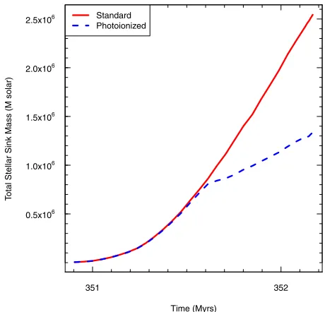
short time-steps within the SPH code. However, a large num-ber of sink particles were able to form and grow in mass un-til they became sources of PI photons. A total stellar mass of 2.54×10⁶ M
forms in the control run within the ≈1.3 Myr which the simulation was evolved for and this is reduced to 1.33 ×10⁶ M
in the MCPI simulation. Even in this short timescale the PI photons are able to strongly affect the star formation in the region. Figure10 shows the cumulative stel-lar mass in this case for the standard and photoionised cases. The mean star formation rate over the simulation falls from
SFRcontrol = 1.94 M yr−1 to SFRMCPI = 1.01 M yr−1. The
sharp decrease in the star formation rate at a time of≈351.6 Myr appear to be caused by the coalescence of the ionised regions around several sources within the centre of the cloud to form one large ionised complex. This effectively ionises the majority of the gas near the sinks and removes the reservoir of star form-ing gas.
6.2. SFRs vs. surface density
In trying to understand the effects of PI feedback on the accretion processes it is useful to compare our results with the observed properties of star forming regions. It has been shown that there is a strong observed link between star formation and the local cold gas density (Schmidt 1963;Kennicutt 1998;Kennicutt & Evans 2012). In the case of disk averaged properties of local galaxies this can be fitted by a power-law relation of the form
ΣSFR =AΣNg, (3)
whereΣSFR is the star formation surface density, Σg the total
[image:6.595.64.539.324.536.2]Time (Myrs)
353 354 355 356
0.5x10⁵ 1.0x10⁵ 1.5x10⁵ 2.0x10⁵
T
otal Stellar Sink Mass (M solar)
[image:7.595.59.275.74.281.2]Standard Photoionized
Fig. 7.Total stellar mass is plotted as a function of time for the standard (red-solid) and photoionised (blue-dashed) simulation. The difference represents the mass of gas that is removed from the star formation pro-cess due to being photoionised.
SFR (M
sun
yr
−
1)
0 0.02 0.04 0.06
0.08 Standard Photoionized
Time (Myrs)
352.5 353 353.5 354 354.5 355 355.5 356
0 0.2 0.4 0.6 0.8 1
Fr
actional change
in SFR
Fig. 8.Star formation rates of the control and MCPI simulations as a function of time.
that predicted by the extragalactic relation (Evans et al. 2009; Heiderman et al. 2010).
Bonnell et al.(2013) found that in the original SPH simula-tions there was a relation betweenΣSFRandΣgwith a power law
indexN = 1.55±0.06 (when the low (0.4 Mpc−2) and high
(40Mpc−2) surface density data is also included). The authors
argue that the relation is a natural consequence of the shock for-mation of the dense, cold gas when cooling in the interstellar medium is included. In Fig.11we show the final instantaneous SFR and neutral gas mass surface density in our photoionisation simulation, as viewed along the three axes of our simulation grid. The contour lines and points show the effects of calculating the relationship within differing sized cells, from 5 pc to an average over the entire region. The values were calculated using grids of neutral gas density and SFR. Each grid was a 2003cube of cells
which we re-gridded to the required cell size before calculating the observed surface densities, as viewed along the three axes of the grid. In this way the entire cloud is covered at each resolu-tion. The red contours show the data averaged over 5 pc cells
Stellar Sink Mass (Msolar)
Number
100 1000
100 1000
[image:7.595.314.547.74.281.2]Standard Photoionized
Fig. 9.Final cumulative stellar mass distributions for the standard (red) and photoionised (blue) runs.
Time (Myrs)
351 352
0.5x10⁶
1.0x10⁶
1.5x10⁶
2.0x10⁶ 2.5x10⁶
T
o
tal Stellar Sink Mass (M solar)
Standard Photoionized
Fig. 10.Cumulative stellar mass as a function of time for the standard (red-solid) and photoionised (blue-dashed) simulation for the SPH sim-ulation with a mean surface density of 40Mpc−2.
[image:7.595.316.546.320.541.2] [image:7.595.51.282.340.524.2]−4 −2 0
2 Cell Size (pc)
200 100 50 25 5
0.1
0.25 0.5
0.95
0.95
Log
Σsfr
( M
solar
yr
−
1 kpc
−
2 )
−4 −2 0 2
0.1
0.25 0.5
0.95
Log Σgas ( Msolar pc−2)
0 0.5 1 1.5 2 2.5 3
−4 −2 0 2
0.1
0.25
0.5
[image:8.595.62.541.76.491.2]0.95
Fig. 11.Surface densities of the star formation rates are plotted as a function of the surface densities of the neutral gas. The three panels represent the simulation as viewed along the three principle axes of the simulation grids. Crosses are observed data from Table 1 ofHeiderman et al.(2010) with the extent of the cross indicting the confidence interval of the data. Coloured points (see key in top left) show the effects of increasing the cell size up to the size of the entire region (200 pc). The dashed line shows the observed extragalactic power-law relation from (Kennicutt 1998) and the blue line the power law fit achieved byBonnell et al.(2013) to theGravitysimulation without PI feedback.
overlap with the observed data ofHeiderman et al.(2010) as well as many which seem to lie at lower gas surface densities.
7. Discussion
From the results shown in Fig.7 it is clear that the total mass accreted onto sinks throughout the simulation is overestimated by standard SPH methods when PI feedback is ignored. The fi-nal total stellar sink mass in the standard surface density simu-lation including photoionisation is reduced by around 23% and the instantaneous SFR is reduced to 62% of its original value at the end of the simulation. This is a significant change and suggests that it is likely very important to include photoionisa-tion effects to accurately model the SFRs and efficiency within SPH simulations.
7.1. Limitations
The techniques outlined here provide a way to provide a first or-der approximation to the feedback provided by high mass stars.
We neglect the dynamical effects of ionised gas that may pro-vide additional forms of feedback due to the restrictions of our simulation.
7.1.1. Triggering of additional star formation
simulations suggest they are likely second order effects (Dale et al. 2012,2013).
There are also additional mechanisms in which the dynam-ical effects of ionised gas can allow the PI feedback to have a greater effect than we estimate here. The penetration of the ion-ising photons into dense regions of gas can be increased due to the streaming of hot ionised gas out of the cloud.Whitworth (1979) andGendelev & Krumholz(2011) explored this scenario and found that the removal of ionised gas allows the ionisation front to penetrate deeper into dense gas and may increase the effects of ionising photons beyond those discussed here.
In addition to assuming a 100% efficient star formation pro-cess the SPH simulation we have studied also neglect several physical processes which are likely to affect the overall star for-mation process. There is no treatment of magnetic fields which may cause a reduction in the star formation rate (Price & Bate 2008;Arthur et al. 2011;McKee 1999) by providing an addi-tional support mechanism to overcome self-gravity and prevent the collapse of less massive clouds to form stars. Self gravity is also not included in the initial disk simulation from which our dense star forming region originates. This will lead to a reduced kinetic energy which, again, will enhance star formation rates. The reduction in the star formation rates caused by the inclusion of such effects may provide a mechanism to move our simulated values into better agreement with observed relations.
We include no source of ionising photons outwith the bounds of our star forming cloud. In reality there will be a non zero background of ionising flux produced by previous bouts of star formation in the galactic disk. The effects of back-ground far-ultraviolet heating are included in the SPH code (Vazquez Semadeni et al. 2006) but without account for the ioni-sation of the gas.Reynolds(1990) found that the diffuse ionised gas (DIG) in our local environment requires a diffuse ionising flux of≈4×10⁻⁵ erg s−1cm−2 to maintain it. This additional
source of PI photons may be able to affect the outer regions of the cloud, but is unlikely to penetrate into the dense cloud centre. While this is unlikely to affect the star formation in the cloud in-terior it may impact the initial stages of cloud formation during compression within the spiral shock.
7.2. Localisation of stellar signatures
We find that the clumpy gas distribution produced by the SPH calculation produces a highly structured complex of HII regions which, due to low density paths, provides an illustration of a pos-sible source of ionising photons required to maintain the DIG seen in the Milky Way and external galaxies. At the final time-step of the simulation our photoionisation code suggests that ≈15% of ionising photons escape into the ISM from this star forming complex. This escape fraction may also be important for observations of Hαas a localised star formation indicator. If a significant fraction of the ionising photons are able to escape the star forming cloud then it also suggests there would be a cor-responding drop in the Hαluminosity. This effect will lead to Hα emission that is non-coincident with the star formation. In turn this may cause deviations from the observed power law relation between star formation and gas surface densities at small scales (Relaño et al. 2012). IndeedSchruba et al.(2010) andOnodera et al.(2010) have found observational evidence of such devia-tions in high spatial resolution studies of the star formation in the nearby spiral galaxy M 33. Based on analysis of CO emis-sion maps and HαimagingSchruba et al.(2010) estimate that the star formation law observed at large scales breaks down at
scales below∼300 pc. It is not possible to verify this effect here due to the size of the region studied.
In this work we have utilized a simple hydrogen only MCPI code but the method we propose can easily be extended to use radiation transfer codes which provide a more realistic treatment of the photoionisation physics (Wood et al. 2004;Ercolano et al. 2008). Our simplified treatment likely only provides a first or-der correction as it focuses on the ionisation of hydrogen and the impact of Lyman continuum photons only, neglecting the ef-fects of Helium as a source of opacity. There is, however, no rea-son that more complex radiation transfer codes which includes these effects could not be added to provide more accurate gas physics at the cost of computation time. The possibility to also self-consistently include calculations of star formation indica-tors, such as Hαand 24μm dust emission would allow the direct comparison with observational data.
8. Summary
We have carried out an investigation into the effects of PI feed-back from massive stars on the growth of stellar clusters in SPH simulations of a dense star forming region within a disk galaxy by utilizing post-completion MCPI calculations. In or-der to quantify the effects of PI photons we track SPH particles which are likely to be ionised during the course of the simula-tion and remove them from stellar sink particles where they have been accreted during the future evolution of the system.
Results indicate that the total stellar mass in sink particles may be reduced by up to 23% due to the action of PI photons emitted form the most massive stars. The final instantaneous SFR is reduced to 62% of its original value.The overall distribu-tion of sink particle masses does not seem to be greatly affected with the most noticeable changes occurring at the high mass end. The maximum sink mass attained is reduced and fewer massive stellar clusters form. As we cannot include the possible dynam-ical feedback effects of the hot ionised gas to trigger additional star formation our results provide an estimate of the maximum impact of PI feedback.
A comparison of our region-averaged properties to ob-served extra-galactic relations and observations of local molecu-lar clouds suggests that our simulations over-predict the star for-mation rate by a factor 2−10. While the inclusion of PI feedback from massive stars is able to reduce the discrepancy between the simulation and observations it cannot fully account for it. We also find that a significant fraction of the PI photons emitted by massive stars in the simulation are able to traverse low density paths and escape the star formation region entirely. This provides a mechanism to produce a fraction of the DIG observed in many galaxies.
Acknowledgements. I.A.B. acknowledges funding from the European Research Council for the FP7 ERC advanced grant project ECOGAL. This research was also supported by the DFG cluster of excellence “Origin and Structure of the Universe” (JED). This research has made use of NASA’s Astrophysics Data System Service.
References
Arthur, S. J., Henney, W. J., Mellema, G., De Colle, F., & Vázquez-Semadeni, E. 2011, MNRAS, 414, 1747
Bally, J., Sutherland, R. S., Devine, D., & Johnstone, D. 1998, AJ, 116, 293 Bate, M. R., Bonnell, I. A., & Price, N. M. 1995, MNRAS, 277, 362 Baumgardt, H., & Kroupa, P. 2007, MNRAS, 380, 1589
Bisbas, T. G., Wünsch, R., Whitworth, A. P., Hubber, D. A., & Walch, S. 2011, ApJ, 736, 142
Conti, P. S., Crowther, P. A., & Leitherer, C. 2008, From Luminous Hot Stars to Starburst Galaxies (Cambridge: Cambridge University Press)
Dale, J. E., & Bonnell, I. 2011, MNRAS, 414, 321
Dale, J. E., Bonnell, I. A., Clarke, C. J., & Bate, M. R. 2005, MNRAS, 358, 291
Dale, J. E., Bonnell, I. A., & Whitworth, A. P. 2007a, MNRAS, 375, 1291 Dale, J. E., Ercolano, B., & Clarke, C. J. 2007b, MNRAS, 382, 1759 Dale, J. E., Ercolano, B., & Bonnell, I. A. 2012, MNRAS, 424, 377 Dale, J. E., Ercolano, B., & Bonnell, I. A. 2013, MNRAS, 1, 925 Deharveng, L., Zavagno, A., & Caplan, J. 2005, A&A, 433, 565 Diaz-Miller, R. I., Franco, J., & Shore, S. N. 1998, ApJ, 501, 192 Dirienzo, W. J., Indebetouw, R., Brogan, C., et al. 2012, AJ, 144, 173 Elmegreen, B. G., & Lada, C. J. 1977, ApJ, 214, 725
Ercolano, B., Young, P. R., Drake, J. J., & Raymond, J. C. 2008, ApJS, 175, 534 Evans, N. J. I., Dunham, M. M., Jørgensen, J. K., et al. 2009, ApJS, 181, 321 Franco, J., Shore, S. N., & Tenorio-Tagle, G. 1994, ApJ, 436, 795
Gendelev, L., & Krumholz, M. R. 2011, ApJ, 745, 1 Goodwin, S. P., & Bastian, N. 2006, MNRAS, 373, 752
Gritschneder, M., Naab, T., Burkert, A., et al. 2009, MNRAS, 393, 21 Heiderman, A., Evans, N. J., Allen, L. E., Huard, T., & Heyer, M. 2010, ApJ,
723, 1019
Hills, J. G. 1980, ApJ, 235, 986
Hollenbach, D. J., Yorke, H. W., & Johnstone, D. 2000, Protostars and Planets IV, eds. V. Mannings, A. P. Boss, & S. S. Russell (Tucson: University of Arizona Press), 401
Kennicutt, R. C. J. 1998, ApJ, 498, 541
Kennicutt, R. C., & Evans, N. J. 2012, ARA&A, 50, 531
Kessel-Deynet, O. & Burkert, A. 2000, MNRAS, 315, 713 Kessel-Deynet, O., & Burkert, A. 2003, MNRAS, 338, 545 Kroupa, P. 2001, MNRAS, 322, 231
Kroupa, P., Tout, C. A., & Gilmore, G. 1993, MNRAS, 262, 545 Krumholz, M. R., McKee, C. F., & Klein, R. I. 2005, ApJ, 618, L33 Lada, C. J., & Lada, E. A. 2003, ARA&A, 41, 57
Lada, E. A., Evans, N. J. I., Depoy, D. L., & Gatley, I. 1991, ApJ, 371, 171 McKee, C. F. 1999, The Origin of Stars and Planetary Systems, eds. C. J. Lada,
& N. D. Kylafis (Kluwer Academic Publishers), 29 Olmi, L., & Testi, L. 2002, A&A, 392, 1053
Onodera, S., Kuno, N., Tosaki, T., et al. 2010, ApJ, 722, L127 Price, D. J., & Bate, M. R. 2008, MNRAS, 385, 1820
Relaño, M., Kennicutt, R. C. J., Eldridge, J. J., Lee, J. C., & Verley, S. 2012, MNRAS, 423, 2933
Reynolds, R. J. 1990, ApJ, 349, L17 Schmidt, M. 1963, ApJ, 137, 758
Schruba, A., Leroy, A. K., Walter, F., Sandstrom, K., & Rosolowsky, E. 2010, ApJ, 722, 1699
Tenorio-Tagle, G. 1979, A&A, 71, 59
Vazquez Semadeni, E., Ryu, D., Passot, T., Gonzalez, R. F., & Gazol, A. 2006, ApJ, 643, 245
Whitworth, A. 1979, MNRAS, 186, 59
Whitworth, A. P., Bhattal, A. S., Chapman, S. J., Disney, M. J., & Turner, J. A. 1994, A&A, 290, 421
Wood, K., & Loeb, A. 2000, ApJ, 545, 86