C
2014. The American Astronomical Society. All rights reserved. Printed in the U.S.A.
A SUPER-JUPITER ORBITING A LATE-TYPE STAR: A REFINED ANALYSIS
OF MICROLENSING EVENT OGLE-2012-BLG-0406
Y. Tsapras1,2,64, J.-Y. Choi3, R. A. Street1,64, C. Han3,65,66, V. Bozza4,67, A. Gould5,66, M. Dominik6,64,67,68,69, J.-P. Beaulieu7,69, A. Udalski8,70, U. G. Jørgensen9,67, T. Sumi10,71,
and
D. M. Bramich11,12, P. Browne6,67, K. Horne6,69, M. Hundertmark6,67, S. Ipatov13,67, N. Kains11,67,
C. Snodgrass14,67, I. A. Steele15
(The RoboNet Collaboration)
K. A. Alsubai13, J. M. Andersen16, S. Calchi Novati4,17, Y. Damerdji18, C. Diehl19,20, A. Elyiv18,21, E. Giannini19,
S. Hardis9, K. Harpsøe22, T. C. Hinse9,23,24, D. Juncher9, E. Kerins25, H. Korhonen9, C. Liebig6, L. Mancini26,
M. Mathiasen9, M. T. Penny5,66, M. Rabus27, S. Rahvar28, G. Scarpetta4,29,30, J. Skottfelt9,22, J. Southworth31,
J. Surdej18, J. Tregloan-Reed31, C. Vilela31, J. Wambsganss19
(The MiNDSTEp Collaboration)
J. Skowron8, R. Poleski5,8,66, S. Kozłlowski8, Ë. Wyrzykowski8,32, M. K. Szyma ´nski8, M. Kubiak8,
P. Pietrukowicz8, G. Pietrzy ´nski8,33, I. Soszy ´nski8, K. Ulaczyk8
(The OGLE Collaboration)
M. D. Albrow34, E. Bachelet35,36, R. Barry37, V. Batista7, A. Bhattacharya38,71, S. Brillant39, J. A. R. Caldwell40, A. Cassan7, A. Cole41, E. Corrales7, Ch. Coutures7, S. Dieters35, D. Dominis Prester42, J. Donatowicz43, P. Fouqu´e35,36,
J. Greenhill41, S. R. Kane44, D. Kubas7,39, J.-B. Marquette7, J. Menzies45, C. P`ere7, K. R. Pollard34, M. Zub19,67 (The PLANET Collaboration)
G. Christie46, D. L. DePoy47, S. Dong48, J. Drummond49, B. S. Gaudi5, C. B. Henderson5, K. H. Hwang3, Y. K. Jung3,
A. Kavka5, J.-R. Koo50, C.-U. Lee50, D. Maoz51, L. A. G. Monard52, T. Natusch46, H. Ngan46, H. Park3, R. W. Pogge5,
I. Porritt53, I.-G. Shin3, Y. Shvartzvald51, T. G. Tan54, J. C. Yee5
(TheμFUN Collaboration)
F. Abe55, D. P. Bennett38, I. A. Bond56, C. S. Botzler57, M. Freeman57, A. Fukui58, D. Fukunaga55, Y. Itow55,
N. Koshimoto10, C. H. Ling56, K. Masuda55, Y. Matsubara55, Y. Muraki55, S. Namba10, K. Ohnishi59, N. J. Rattenbury57,
To. Saito60, D. J. Sullivan61, W. L. Sweatman56, D. Suzuki10, P. J. Tristram62, N. Tsurumi55, K. Wada10, N. Yamai63,
P. C. M. Yock57, and A. Yonehara63
(The MOA Collaboration)
1Las Cumbres Observatory Global Telescope Network, 6740 Cortona Drive, Suite 102, Goleta, CA 93117, USA 2School of Physics and Astronomy, Queen Mary University of London, Mile End Road, London E1 4NS, UK
3Department of Physics, Chungbuk National University, Cheongju 361-763, Korea
4Dipartimento di Fisica “E. R. Caianiello,” Universit`a di Salerno, Via Giovanni Paolo II n. 132, I-84084 Fisciano (SA), Italy 5Department of Astronomy, Ohio State University, 140 West 18th Avenue, Columbus, OH 43210, USA
6SUPA, School of Physics & Astronomy, University of St Andrews, North Haugh, St Andrews KY16 9SS, UK 7UPMC-CNRS, UMR7095, Institut d’Astrophysique de Paris, 98bis boulevard Arago, F-75014 Paris, France
8Warsaw University Observatory, Al. Ujazdowskie 4, 00-478 Warszawa, Poland
9Niels Bohr Institute, Astronomical Observatory, Juliane Maries vej 30, DK-2100 Copenhagen, Denmark 10Department of Earth and Space Science, Osaka University, Osaka 560-0043, Japan 11European Southern Observatory, Karl-Schwarzschild-Str. 2, D-85748 Garching bei M¨unchen, Germany 12Qatar Environment and Energy Research Institute, Qatar Foundation, Tornado Tower, Floor 19, P.O. Box 5825, Doha, Qatar
13Qatar Foundation, P.O. Box 5825, Doha, Qatar
14Max Planck Institute for Solar System Research, Max-Planck-Str. 2, D-37191 Katlenburg-Lindau, Germany 15Astrophysics Research Institute, Liverpool John Moores University, Liverpool CH41 1LD, UK 16Astronomy Department, Boston University, 725 Commonwealth Avenue, Boston, MA 02215, USA
17Istituto Internazionale per gli Alti Studi Scientifici (IIASS), I-84019 Vietri Sul Mare (SA), Italy 18Institut d’Astrophysique et de G´eophysique, All´ee du 6 Aoˆut 17, Sart Tilman, Bˆat. B5c, B-4000 Li´ege, Belgium
19Astronomisches Rechen-Institut, Zentrum f¨ur Astronomie der Universit¨at Heidelberg (ZAH), M¨onchhofstr. 12-14, D-69120 Heidelberg, Germany 20Hamburger Sternwarte, Universit¨at Hamburg, Gojenbergsweg 112, D-21029 Hamburg, Germany
21Main Astronomical Observatory, Academy of Sciences of Ukraine, vul. Akademika Zabolotnoho 27, 03680 Kyiv, Ukraine 22Centre for Star and Planet formation, Geological Museum, Øster Voldgade 5, DK-1350, Copenhagen, Denmark
23Armagh Observatory, College Hill, Armagh, BT61 9DG, UK
24Korea Astronomy and Space Science Institute, 776 Daedukdae-ro, Yuseong-gu, Daejeon 305-348, Korea 25Jodrell Bank Centre for Astrophysics, University of Manchester, Oxford Road, Manchester, M13 9PL, UK
26Max Planck Institute for Astronomy, K¨onigstuhl 17, D-69117 Heidelberg, Germany
27Instituto de Astrof´ısica, Facultad de F´ısica, Pontificia Universidad Cat´olica de Chile, Av. Vicu˜na Mackenna 4860, 7820436 Macul, Santiago, Chile 28Department of Physics, Sharif University of Technology, P.O. Box 11155-9161, Tehran, Iran
29International Institute for Advanced Scientific Studies (IIASS), I-84019 Vietri sul Mare, (SA), Italy 30INFN, Gruppo Collegato di Salerno, Sezione di Napoli, Italy
31Astrophysics Group, Keele University, Staffordshire, ST5 5BG, UK
32Institute of Astronomy, University of Cambridge, Madingley Road, Cambridge CB3 0HA, UK 33Departamento de Astronomia, Universidad de Concepci´on, Casilla 160-C, Concepci´on, Chile
36CNRS, IRAP, 14 avenue Edouard Belin, F-31400 Toulouse, France
37Laboratory for Exoplanets and Stellar Astrophysics, Mail Code 667, NASA/GSFC, Bldg 34, Room E317, Greenbelt, MD 20771, USA 38Department of Physics, University of Notre Dame, 225 Nieuwland Science Hall, Notre Dame, IN 46556-5670, USA
39European Southern Observatory (ESO), Alonso de Cordova 3107, Casilla 19001, Santiago 19, Chile 40McDonald Observatory, 16120 Street Highway Spur 78 #2, Fort Davis, TX 79734, USA 41School of Math and Physics, University of Tasmania, Private Bag 37, GPO Hobart, 7001 Tasmania, Australia 42Physics Department, Faculty of Arts and Sciences, University of Rijeka, Omladinska 14, 51000 Rijeka, Croatia
43Department of Computing, Technical University of Vienna, Wiedner Hauptstrasse 10, Vienna, Austria
44Department of Physics & Astronomy, San Francisco State University, 1600 Holloway Avenue, San Francisco, CA 94132, USA 45South African Astronomical Observatory, P.O. Box 9, Observatory 7935, South Africa
46Auckland Observatory, Auckland, New Zealand
47Department of Physics and Astronomy, Texas A&M University, College Station, TX 77843, USA
48Kavli Institute for Astronomy and Astrophysics, Peking University, Yi He Yuan Road 5, Hai Dian District, Beijing 100871, China 49Possum Observatory, Patutahi, Gisbourne, New Zealand
50Korea Astronomy and Space Science Institute, Daejeon 305-348, Korea 51School of Physics and Astronomy, Tel-Aviv University, Tel-Aviv 69978, Israel 52Klein Karoo Observatory, Calitzdorp, and Bronberg Observatory, Pretoria, South Africa
53Turitea Observatory, Palmerston North, New Zealand 54Perth Exoplanet Survey Telescope, Perth, Australia
55Solar-Terrestrial Environment Laboratory, Nagoya University, Nagoya 464-8601, Japan
56Institute of Information and Mathematical Sciences, Massey University, Private Bag 102-904, North Shore Mail Centre, Auckland, New Zealand 57Department of Physics, University of Auckland, Private Bag 92-019, Auckland 1001, New Zealand
58Okayama Astrophysical Observatory, National Astronomical Observatory of Japan, Asakuchi, Okayama 719-0232, Japan 59Nagano National College of Technology, Nagano 381-8550, Japan
60Tokyo Metropolitan College of Aeronautics, Tokyo 116-8523, Japan
61School of Chemical and Physical Sciences, Victoria University, Wellington, New Zealand 62Mt. John University Observatory, P.O. Box 56, Lake Tekapo 8770, New Zealand 63Department of Physics, Faculty of Science, Kyoto Sangyo University, 603-8555 Kyoto, Japan
Received 2013 October 9; accepted 2013 December 4; published 2014 January 27
ABSTRACT
We present a detailed analysis of survey and follow-up observations of microlensing event OGLE-2012-BLG-0406 based on data obtained from 10 different observatories. Intensive coverage of the light curve, especially the perturbation part, allowed us to accurately measure the parallax effect and lens orbital motion. Combining our measurement of the lens parallax with the angular Einstein radius determined from finite-source effects, we estimate the physical parameters of the lens system. We find that the event was caused by a 2.73±0.43MJplanet orbiting a
0.44±0.07Mearly M-type star. The distance to the lens is 4.97±0.29 kpc and the projected separation between the host star and its planet at the time of the event is 3.45±0.26 AU. We find that the additional coverage provided by follow-up observations, especially during the planetary perturbation, leads to a more accurate determination of the physical parameters of the lens.
Key words: binaries: general – gravitational lensing: micro – planetary systems Online-only material:color figures
1. INTRODUCTION
Radial velocity and transit surveys, which primarily target main-sequence stars, have already discovered hundreds of giant planets and are now beginning to explore the reservoir of lower mass planets with orbit sizes extending to a few astronomical units (AUs). These planets mostly lie well inside the snow line72 of their host stars. Meanwhile, direct imaging with large aperture telescopes has been discovering giant planets tens to hundreds of AUs away from their stars (Kalas et al.2005). The region of sensitivity of microlensing lies somewhere in between and extends to low-mass exoplanets lying beyond the snow line of
64The RoboNet Collaboration. 65Corresponding author. 66TheμFUN Collaboration. 67The MiNDSTEp Collaboration.
68Royal Society University Research Fellow. 69The PLANET Collaboration.
70The OGLE Collaboration. 71The MOA Collaboration.
72 The snow line is defined as the distance from the star in a protoplanetary disk where ice grains can form (Lecar et al.2006).
their low-mass host stars, between∼1 and 10 AU (Tsapras et al. 2003; Gaudi2012). Although there is already strong evidence that cold sub-Jovian planets are more common than originally thought around low-mass stars (Gould et al.2006; Sumi et al. 2010; Kains et al.2013; Batalha et al.2013), cold super-Jupiters orbiting K or M dwarfs were believed to be a rarer class of objects73(Laughlin et al.2004; Miguel et al.2011; Cassan et al.
2012).
Both gravitational instability and core accretion models of planetary formation have a hard time generating these planets, although it is possible to produce them given appropriate initial conditions. The main argument against core accretion is that it takes too long to produce a massive planet but this crucially depends on the core mass and the opacity of the planet envelope during gas accretion. In the case of gravitational instability, a massive protoplanetary disc would probably have too high an opacity to fragment locally at distances of a few AU.
The radial velocity method has been remarkably successful in tabulating the part of the distribution that lies within the snow
line, but discoveries of super-Jupiters beyond the snow line of M dwarfs have been comparatively few (Johnson et al.2010; Montet et al. 2013). Since microlensing is most sensitive to planets that are further away from their host stars, typically M and K dwarfs, the two techniques are complementary (Gaudi
2012).
Three brown dwarf and 19 planet microlensing discoveries have been published to date, including the discoveries of two multiple-planet systems (Gaudi et al.2008; Han et al.2013).74 It is also worth noting that unbound objects of planetary mass have also been reported (Sumi et al.2011).
Microlensing involves the chance alignment along an ob-server’s line of sight of a foreground object (lens) and a back-ground star (source). This results in a characteristic variation of the brightness of the background source as it is being grav-itationally lensed. As seen from the Earth, the brightness of the source increases as it approaches the lens, reaching a maxi-mum value at the time of closest approach. The brightness then decreases again as the source moves away from the lens.
In microlensing events, planets orbiting the lens star can re-veal their presence through distortions in the otherwise smoothly varying standard single lens light curve. Together, the host star and planet constitute a binary lens. Binary lenses have a mag-nification pattern that is more complex than the single lens case due to the presence of extended caustics that represent the po-sitions on the source plane at which the lensing magnification diverges. Distortions in the light curve arise when the trajectory of the source star approaches (or crosses) the caustics (Mao & Paczy´nski1991). Recent reviews of the method can be found in Dominik (2010) and Gaudi (2011).
Upgrades to the OGLE75 (Udalski 2003) survey observing setup and MOA76 (Sumi et al. 2003) microlensing survey telescope in the past couple of years brought greater precision and enhanced observing cadence, resulting in an increased rate of exoplanet discoveries. For example, the Optical Gravitational Lensing Experiment (OGLE) has regularly been monitoring the field of the OGLE-2012-BLG-0406 event since 2010 March with a cadence of 55 minutes. When a microlensing alert was issued notifying the astronomical community that event OGLE-2012-BLG-0406 was exhibiting anomalous behavior, intense follow-up observations from multiple observatories around the world were initiated in order to better characterize the deviation. This event was first analyzed by Poleski et al. (2013) using the OGLE-IV survey photometry exclusively. That study concluded that the event was caused by a planetary system consisting of a 3.9± 1.2MJ planet orbiting a low-mass late
K/early M dwarf.
In this paper, we present the analysis of the event based on the combined data obtained from 10 different telescopes, spread out in longitude, providing dense and continuous coverage of the light curve.
The paper is structured as follows. Details of the discov-ery of this event, follow-up observations and image analysis procedures are described in Section2. Section 3 presents the methodology of modeling the features of the light curve. We provide a summary and conclude in Section4.
74 For a complete list, consulthttp://exoplanet.eu/catalog/and references therein.
75 http://ogle.astrouw.edu.pl
76 http://www.phys.canterbury.ac.nz/moa
2. OBSERVATIONS AND DATA
Microlensing event OGLE-2012-BLG-0406 was discovered at equatorial coordinatesα=17h53m18.s17,δ = −30◦2816.2
(J2000.0)77 by the OGLE-IV survey and announced by their Early Warning System (EWS)78 on 2012 April 6. The event had a baseline I-band magnitude of 16.35 and was gradually increasing in brightness. The predicted maximum magnification at the time of announcement was low, therefore the event was considered a low-priority target for most follow-up teams who preferentially observe high-magnification events as they are associated with a higher probability of detecting planets (Griest & Safizadeh1998).
OGLE observations of the event were carried out with the 1.3-m Warsaw telescope at the Las Campanas Observatory, Chile, equipped with the 32 chip mosaic camera. The event’s field was visited every 55 minutes, providing very dense and precise coverage of the entire light curve from the baseline back to the baseline. For more details on the OGLE data and coverage, see Poleski et al. (2013).
An assessment of data acquired by the OGLE team until 1 July (08:47 UT, HJD∼2456109.87), which was carried out by the SIGNALMEN anomaly detector (Dominik et al.2007) on 2 July (02:19 UT) concluded that a microlensing anomaly, i.e., a deviation from the standard bell-shaped Paczy´nski curve (Paczy´nski 1986), was in progress. This was electronically communicated via the ARTEMiS (Automated Robotic Terres-trial Exoplanet Microlensing Search) system (Dominik et al. 2008) to trigger prompt observations by both the RoboNet-II79 collaboration (Tsapras et al.2009) and the MiNDSTEp80 con-sortium (Dominik et al.2010). RoboNet’s web-PLOP system (Horne et al.2009) reacted to the trigger by scheduling observa-tions already from 2 July (02:30 UT), just 11 minutes after the SIGNALMEN assessment started. However, the first RoboNet observations did not occur before 4 July (15:26 UT), when the event was observed with the Faulkes Telescope South (FTS). This delayed response was due to the telescopes being offline for engineering work and bad weather at the observing sites. It fell to the Danish 1.54m at ESO La Silla to provide the first data point following the anomaly alert (2 July, 03:42 UT) as part of the MiNDSTEp efforts. The alert also triggered automated anomaly modeling by RTModel (Bozza2010), which by 2 July (04:22 UT) delivered a rather broad variety of solutions in the stellar binary or planetary range, reflecting the fact that the true nature was not well-constrained by the data available at that time. This process chain did not involve any human interaction at all.
The first human involvement was an e-mail circulated to all microlensing teams by V. Bozza on 2 July (07:26 UT) informing the community about the ongoing anomaly and modeling results. Including OGLE data from a subsequent night, the apparent anomaly was also independently spotted by E. Bachelet (e-mail by D. P. Bennett 3 July, 13:42 UT), and subsequently PLANET81 team (Beaulieu et al. 2006) SAAO data as well asμFUN82 (Gould et al.2006) SMARTS (CTIO) data were acquired the coming night, which, along with the RoboNet FTS data, cover the main peak of the anomaly. It
77 (l, b)= −0.◦46,−2◦.22
78 http://ogle.astrouw.edu.pl/ogle4/ews/ews.html 79 http://robonet.lcogt.net
80 http://www.mindstep-science.org 81 http://planet.iap.fr
Table 1
Observations
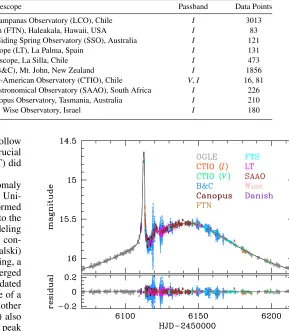
Group Telescope Passband Data Points
OGLE 1.3m Warsaw Telescope, Las Campanas Observatory (LCO), Chile I 3013
RoboNet 2.0m Faulkes Telescope North (FTN), Haleakala, Hawaii, USA I 83
RoboNet 2.0m Faulkes Telescope South (FTS), Siding Spring Observatory (SSO), Australia I 121
RoboNet 2.0m Liverpool Telescope (LT), La Palma, Spain I 131
MiNDSTEp 1.5m Danish Telescope, La Silla, Chile I 473
MOA 0.6m Boller & Chivens (B&C), Mt. John, New Zealand I 1856
μFUN 1.3m SMARTS, Cerro Tololo Inter-American Observatory (CTIO), Chile V,I 16, 81
PLANET 1.0m Elizabeth Telescope, South African Astronomical Observatory (SAAO), South Africa I 226
PLANET 1.0m Canopus Telescope, Mt. Canopus Observatory, Tasmania, Australia I 210
WISE 1.0m Wise Telescope, Wise Observatory, Israel I 180
should be noted that the observers at CTIO decided to follow the event even while the moon was full in order to obtain crucial data. A model circulated by T. Sumi on 5 July (00:38 UT) did not distinguish between the various solutions.
However, when the rapidly changing features of the anomaly were independently assessed by the Chungbuk National Uni-versity group (CBNU, C. Han), the community was informed on 5 July (10:43 UT) that the anomaly is very likely due to the presence of a planetary companion. An independent modeling run by V. Bozza’s automatic software (5 July, 10:55 UT) con-firmed the result. While the OGLE collaboration (A. Udalski) notified observers on 5 July that a caustic exit was occurring, a geometry leading to a further small peak successively emerged from the models. D.P. Bennett circulated a model using updated data on 6 July (00:14 UT) which highlighted the presence of a second prominent feature expected to occur∼10 July. Another modeling run performed at CBNU on 7 July (02:39 UT) also identified this feature and estimated that the secondary peak would occur on 11 July.
Follow-up teams continued to monitor the progress of the event intensively until the beginning of September, well after the planetary deviation had ceased, and provided dense coverage of the main peak of the event. A preliminary model using available OGLE and follow-up data at the time circulated on 31 October (C. Han, J.-Y. Choi), classified the companion to the lens as a super-Jupiter. Poleski et al. (2013) presented an analysis of this event using reprocessed survey data exclusively. In this paper, we present a refined analysis using survey and follow-up data together.
The groups that contributed to the observations of this event, along with the telescopes used, are listed in Table 1. Most observations were obtained in theIband and some images were also taken in other bands in order to create a color–magnitude diagram and classify the source star. We note that there are also observations obtained from the MOA 1.8m survey telescope, which we did not include in our modeling because the target was very close to the edge of the CCD. We also do not include data from theμFUN Auckland 0.4m, PEST 0.3m, Possum 0.36m, and Turitea 0.36m telescopes due to poor observing conditions at the sites.
Extracting accurate photometry from observations of crowded fields, such as the Galactic Bulge, is a challenging process. Each image contains thousands of stars whose stel-lar point spread functions (PSFs) often overlap so aperture and PSF-fitting photometry can at best offer limited precision. In or-der to optimize the photometry, it is necessary to use difference imaging (DI) techniques (Alard & Lupton1998). For any partic-ular telescope/camera combination, DI uses a reference image of the event taken under optimal seeing conditions which is then
Figure 1.Light curve of OGLE-2012-BLG-0406 showing our best-fit binary-lens model including parallax and orbital motion. The legend on the right of the figure lists the contributing telescopes. All data were taken in theIband, except where otherwise indicated.
(A color version of this figure is available in the online journal.)
degraded to match the seeing conditions of every other image of the event taken from that telescope. The degraded reference image is then subtracted from the matching image to produce a residual (or difference) image. Stars that have not varied in brightness in the time interval between the two images will can-cel, leaving no systematic residuals on the difference image but variable stars will leave either a positive or negative residual.
DI is the preferred method of photometric analysis among microlensing groups and each group has developed custom pipelines to reduce their observations. OGLE and MOA im-ages were reduced using the pipelines described in Udalski (2003) and Bond et al. (2001), respectively. PLANET,μFUN, andWISEimages were processed using variants of the PySIS (Albrow et al. 2009) pipeline, whereas RoboNet and MiND-STEp observations were analyzed using customized versions of the DanDIA package (Bramich2008). Once the source star re-turned to its baseline magnitude, each data set was reprocessed to optimize photometric precision. These photometrically opti-mized data sets were used as input for our modeling run.
3. MODELING
from the standard Paczy´nski curve. The first feature, which peaked at HJD ∼ 2456112 (3 July), is produced by the source trajectory grazing the cusp of a caustic. The brightness then quickly drops as the source moves away from the cusp (Schneider & Weiss1992; Zakharov1995), increases again for a brief period as it passes close to another cusp at HJD ∼ 2456121 (12 July), and eventually returns to the standard shape as the source moves further away from the caustic structure. The anomalous behavior, when both features are considered, lasts for a total of∼15 days, while the full duration of the event is120 days. These are typical light curve features expected from lensing phenomena involving planetary lenses.
We begin our analysis by exploring a standard set of solutions that involve modeling the event as a static binary lens. The Paczy´nski curve representing the evolution of the event for most of its duration is described by three parameters: the time of closest approach between the projected position of the source on the lens plane and the position of the lens photocenter,83t
0, the
minimum impact parameter of the source,u0, expressed in units
of the angular Einstein radius of the lens (θE), and the duration
of time,tE (the Einstein timescale), required for the source to
crossθE. The binary nature of the lens requires the introduction
of three extra parameters: The mass ratioq between the two components of the lens; their projected separations, expressed in units ofθE; and the source trajectory angleαwith respect to
the axis defined by the two components of the lens. A seventh parameter,ρ∗, representing the source radius normalized by the angular Einstein radius is also required to account for finite-source effects that are important when the finite-source trajectory approaches or crosses a caustic (Ingrosso et al.2009).
The magnification pattern produced by binary lenses is very sensitive to variations in s, q, which are the parameters that affect the shape and orientation of the caustics, andα, the source trajectory angle. Even small changes in these parameters can produce extreme changes in magnification as they may result in the trajectory of the source approaching or crossing a caustic (Dong et al.2006,2009a). On the other hand, changes in the other parameters cause the overall magnification pattern to vary smoothly.
To assess how the magnification pattern depends on the parameters, we start the modeling run by performing a hybrid search in parameter space whereby we explore a grid of s, q,and α values and optimize t0, u0, tE, and ρ∗ at each grid point by χ2 minimization using Markov Chain Monte Carlo (MCMC). Our grid limits are set at−1 logs 1, −5 logq 1, and 0α <2π, which are wide enough to guarantee that all local minima in parameter space have been identified. An initial MCMC run provides a map of the topology of the χ2 surface, which is subsequently further refined by
gradually narrowing down the grid parameter search space (Shin et al.2012a; Street et al.2013). Once we know the approximate locations of the local minima, we perform aχ2 optimization
using all seven parameters at each of those locations in order to determine the refined position of the minimum. From this set of local minima, we identify the location of the global minimum
83 The “photocenter” refers to the center of the lensing magnification pattern. For a binary lens with a projected separation between the lens components less than the Einstein radius of the lens, the photocenter corresponds to the center of mass. For a lens with a separation greater than the Einstein radius, there exist two photocenters, each of which is located close to each lens component with an offsetq/[s(1 +q)] toward the other lens component (Kim et al.2009). In this case, the referencet0, u0measurement is obtained from the photocenter to which the source trajectory approaches closest.
and check for the possible existence of degenerate solutions. We find no other solutions.
Since our analysis relies on data sets obtained from different telescopes and instruments that use different estimates for the reported photometric precision, we normalize the flux uncertainties of each data set by adjusting them as ei =
fi(σ02+σi2)1/2, wherefi is a scale factor,σ0 are the originally
reported uncertainties, and σi is an additive uncertainty term
for each data set i. The rescaling ensures that χ2 per degree
of freedom (χ2/dof) for each data set relative to the model becomes unity. Data points with very large uncertainties and obvious outliers are also removed in the process.
In computing finite-source magnifications, we take into ac-count the limb darkening of the source by modeling the surface brightness asSλ(ϑ)∝1−Γλ(1–1.5 cosϑ) (Albrow et al.2001),
whereϑis the angle between the line of sight toward the source star and the normal to the source surface, andΓλis the
limb-darkening coefficient in passbandλ. We adoptΓV =0.74 and
ΓI =0.53 from the Claret (2000) tables. These values are based
on our classification of the stellar type of the source, as subse-quently described.
The residuals contained additional smooth structure that the static binary model did not account for. This indicated the need to consider additional second-order effects. The event lasted for120 days, so the positional change of the observer caused by the orbital motion of the Earth around the Sun may have affected the lensing magnification. This introduces subtle long-term perturbations in the event light curve by causing the apparent lens-source motion to deviate from a rectilinear trajectory (Gould 1992; Alcock et al. 1995). Modeling this parallax effect requires the introduction of two extra parameters, πE,N and πE,E, representing the components of the parallax vectorπEprojected on the sky along the north and east equatorial
axes, respectively. When parallax effects are included in the model, we use the geocentric formalism of Gould et al. (2004), which ensures that the parameterst0,u0, andtE will be almost
the same as when the event is fitted without parallax.
An additional effect that needs to be considered is the orbital motion of the lens system. The lens orbital motion causes the shape of the caustics to vary with time. To a first-order approximation, the orbital effect can be modeled by introducing two extra parameters that represent the rate of change of the normalized separation between the two lensing components
ds/dt and the rate of change of the source trajectory angle
relative to the causticsdα/dt (Albrow et al.2000).
We conduct further modeling considering each of the higher-order effects separately and also model their combined effect. Furthermore, for each run considering a higher-order effect, we test models with u0 > 0 andu0 < 0 that form a pair of
degenerate solutions resulting from the mirror-image symmetry of the source trajectory with respect to the binary lens axis. For each model, we repeat our calculations starting from different initial positions in parameter space to verify that the fits converge to our previous solution and that there are no other possible minima.
Table 2 lists the optimized parameters for the models we considered. We find that higher-order effects contribute strongly to the shape of the light curve. The model including the parallax effect provides a better fit than the standard model by Δχ2 = 243.3. The orbital effect also improves the fit by Δχ2 = 512.8. The combination of both parallax and orbital
effects improves the fit byΔχ2 = 563.3. Due to the u0 > 0
Table 2
Lensing Parameters
Parameters Standard Parallax Orbit Orbit+Parallax
u0>0 u0<0 u0>0 u0<0 u0>0 u0<0
χ2/dof 6921.019/6383 6850.358/6381 6677.685/6381 6408.371/6381 6408.255/6381 6357.680/6379 6381.358/6379 t0(HJD’) 6141.63±0.04 6141.70±0.05 6141.66±0.05 6141.24±0.05 6141.28±0.04 6141.33±0.05 6141.19±0.06 u0 0.532±0.001 0.527±0.001 −0.520±0.001 0.500±0.002 −0.499±0.002 0.496±0.002 −0.497±0.002
tE(days) 62.37±0.06 63.75±0.18 69.39±0.32 65.33±0.20 65.53±0.15 64.77±0.19 61.91±0.42
s 1.346±0.001 1.345±0.001 1.341±0.001 1.300±0.002 1.301±0.001 1.301±0.002 1.296±0.002
q(10−3) 5.33±0.04 5.07±0.03 4.45±0.04 6.97±0.27 6.63±0.05 5.92±0.11 6.82±0.19
α 0.852±0.001 0.864±0.002 −0.906±0.002 0.861±0.002 −0.859±0.001 0.837±0.002 −0.810±0.005
ρ∗(10−2) 1.103±0.008 1.053±0.007 0.968±0.009 1.233±0.031 1.194±0.011 1.111±0.014 1.207±0.023
πE,N . . . 0.118±0.011 −0.414±0.016 . . . . . . −0.143±0.018 0.358±0.042
πE,E . . . −0.033±0.007 −0.069±0.009 . . . . . . 0.047±0.007 0.008±0.006
ds/dt(yr−1) . . . . . . . . . 0.765±0.046 0.727±0.017 0.669±0.028 0.802±0.033
dα/dt(yr−1) . . . . . . . . . 1.284±0.159 −1.108±0.019 0.497±0.059 −0.732±0.085
Note.HJD’=HJD-2450000.
motion + parallax model, which have similarχ2values. Models
involving the xallarap effect (source orbital motion) were also considered, but they did not outperform equivalent models involving only parallax.
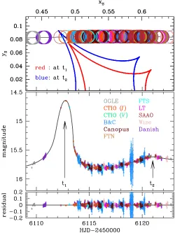
In Figure 1, we present the best-fit model light curve su-perposed on the observed data. Figure2 displays an enlarged view of the perturbation region of the light curve along with the source trajectory with respect to the caustic. The follow-up ob-servations cover critical features of the perturbation regions that were not covered by the survey data. We note that the caustic varies with time and thus we present the shape of the caustic at the times of the first (t1=HJD∼2456112) and second
pertur-bations (t2=HJD∼2456121). The source trajectory grazes the
caustic structure att1causing a substantial increase in
magnifi-cation. As the caustic structure and trajectory evolve with time, the trajectory approaches another cusp att2, but does not cross
it. This second approach causes an increase in magnification that is appreciably lower than that of the first encounter att1.
The source trajectory is curved due to the combination of the parallax and orbital effects.
The mass and distance to the lens are determined by
Mtot=
θE
κπE;
DL=
AU πEθE+πS
, (1)
where κ = 4G/(c2AU) and πS is the parallax of the source
star (Gould1992). To determine these physical quantities, we require the values ofπEandθE. Modeling the event returns the
value ofπE, whereasθE=θ∗/ρ∗depends on the angular radius
of the source star, θ∗, and the normalized source radius, ρ∗, which is also returned from modeling (see Table2). Therefore, determiningθErequires an estimate ofθ∗.
To estimate the angular source radius, we use the standard method described in Yoo et al. (2004). In this procedure, we first measure the de-reddened color and brightness of the source star by using the centroid of the giant clump as a reference because its de-reddened magnitudeI0,c=14.45 (Nataf et al.2013) and
color (V−I)0,c =1.06 (Bensby et al.2011) are already known.
For this calibration, we use a color–magnitude diagram obtained from CTIO observations in theIandVbands. We then convert theV−Isource color toV−Kusing the color–color relations from Bessell & Brett (1988) and the source radius is obtained from theθ∗−(V −K) relations of Kervella et al. (2004). We
Figure 2.Bottom panel zooms in on the anomalous region of the light curve presented in Figure1. Top panel displays the source trajectory, color coded for the individual contributions of each observatory and caustic structure at two different times corresponding to the first and second peaks of the anomaly. All scales are normalized byθE, and the size of the circles corresponds to the size of the source. The first peak deviates the strongest. This is a result of the trajectory of the source grazing the cusp of the caustic att1(HJD∼2456112), shown in red. The second deviation att2(HJD∼2456121) is significantly weaker and is due to the source trajectory passing close to another cusp of the caustic, shown in blue. The differences in the shape of the caustic shown att1andt2are due to the orbital motion of the lens planet system.
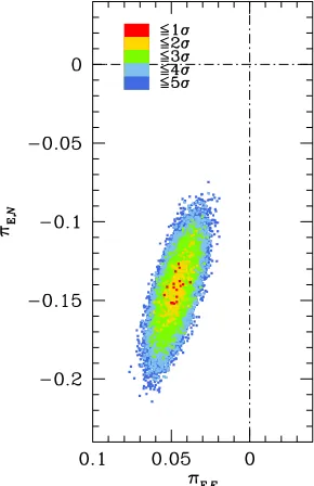
[image:6.612.318.568.282.615.2]Figure 3.Δχ2contours for the parallax parameters derived from our MCMC fits for the best binary lens model including orbital motion and the parallax effect.
(A color version of this figure is available in the online journal.)
derive the de-reddened magnitude and color of the source star as I0=14.62 and (V−I)0=1.12, respectively. This confirms that
the source star is an early K-type giant. The estimated angular source radius is θ∗ = 5.94±0.51μas. Combining this with our evaluation ofρ∗, we obtainθE =0.53±0.05 mas for the
angular Einstein radius of the lens.
Our analysis is consistent with the results of Poleski et al. (2013). We confirm that the lens is a planetary system composed of a giant planet orbiting a low-mass star and we report the refined parameters of the system. Poleski et al. (2013) reported that there existed a pair of degenerate solutions withu0>0 and u0 <0, although the positiveu0 solution is slightly preferred
withΔχ2=13.6. We find a consistent result that the positiveu 0
solution is preferred but the degeneracy is better discriminated byΔχ2=23.7.
The error contours of the parallax parameters for the best-fit model are presented in Figure3. The uncertainty of each param-eter is dparam-etermined from the distribution of MCMC chain, and the reported uncertainty corresponds to the standard deviation of the distribution. We list the physical parameters of the system in Table3and their posterior probability distributions are shown in Figure4.
The lens liesDL =4.97±0.29 kpc away in the direction
of the Galactic Bulge. The more massive component of the lens has massM =0.44±0.07M, so it is an early M-type
dwarf star and its companion is a super-Jupiter planet with a massMp =2.73±0.43MJ. The projected separation between
the two components of the lens is d⊥ = 3.45±0.26 AU. The geocentric relative proper motion between the lens and the source is μGeo = θE/tE = 3.02±0.26 mas yr−1. In the
heliocentric frame, the proper motion isμHelio =(μN, μE) =
(−2.91±0.26,1.31±0.16) mas yr−1.
We note that the derived physical lens parameters are some-what different from those of Poleski et al. (2013). Specifically, the mass of the host star derived in Poleski et al. (2013) is 0.59M, which is∼34% greater than our estimate. Half of this difference comes from the slightly larger Einstein radius
ob-Table 3
Physical Parameters
Parameters Quantity
Mass of the host star (M) 0.44±0.07M
Mass of the planet (Mp) 2.73±0.43MJ Distance to the lens (DL) 4.97±0.29 kpc Projected star-planet separation (d⊥) 3.45±0.26 AU
Einstein radius (θE) 0.53±0.05 mas
Geocentric proper motion (μGeo) 3.02±0.26 mas yr−1
tained by Poleski et al. (2013) from the OGLE-IV photometry and the remaining part from the slightly largerπE,Ncomponent of the parallax obtained from modeling the survey and follow-up photometry as presented in this paper. It should be noted that the parameters derived by both our and the Poleski et al. (2013) models are consistent within the 1σ level.
To further check the consistency between our model and that of Poleski et al. (2013), we conducted additional modeling based on different combinations of data sets. We first test a model based on OGLE data exclusively in order to see whether we can retrieve the physical parameters reported in Poleski et al. (2013). From this modeling, we derive physical parameters consistent with those of Poleski et al. (2013), indicating that the differences are due to the additional coverage provided by the follow-up observations. We conducted another modeling run using OGLE observations, but also included CTIO, FTS, and SAAO data, i.e., those data sets covering the anomalous peak. This modeling run resulted in physical parameters that are consistent with the values extracted from fitting all combined data together, as reported in this paper. This indicates that the differences between Poleski et al. (2013) and this analysis, although consistent within the 1σ level, come mainly from follow-up data that provide better coverage of the perturbation. Therefore, using survey and follow-up data together, we arrive at a more accurate determination of theρandπE,Nparameters, which leads to a refinement of the physical parameters of the planetary system.
4. CONCLUSIONS
Microlensing event OGLE-2012-BLG-0406 was intensively observed by survey and follow-up groups using 10 different telescopes around the world. Anomalous deviations observed in the light curve were recognized to be due to the presence of a planetary companion even before the event reached its central peak. The anomalous behavior was first identified and assessed automatically via software agents. Most follow-up teams re-sponded to these alerts by adjusting their observing strategies accordingly. This highlights the importance of circulating early models to the astronomical community that help to identify im-portant targets for follow-up observations (Shin et al.2012b). There are∼100 follow-up alerts circulated annually,∼10% of which turn out to be planet candidates.
Our analysis of the combined data is consistent with the results of Poleski et al. (2013) and we report the refined parameters of the system. We find that this refinement is mainly due to follow-up observations over the anomaly. The primary lens with massM=0.44±0.07Mis orbited by a planetary
companion with mass Mp = 2.73±0.43 MJ at a projected
separation ofd⊥ =3.45±0.26 AU. The distance to the system isDL=4.97±0.29 kpc in the direction of the Galactic Bulge.
[image:7.612.96.241.56.280.2]Figure 4.Physical parameter uncertainties pertaining to the lens as derived from the MCMC runs optimizing our binary lens model including parallax and orbital motion for theu0>0 trajectory.
Batista et al.2011; Yee et al.2012) and the first such system whose characteristics were derived solely from microlensing data, without considering any external information.
Microlensing is currently the only way to obtain high preci-sion mass measurements for this type of system. Radial velocity, in addition to themsin i degeneracy, at present does not have long enough data streams to measure the parameters of such sys-tems. However, recently Montet et al. (2013) have developed a promising new method to discover them using a combination of radial velocity and direct imaging. They identify long term trends in radial velocity data and use adaptive optics imaging to rule out the possibility that these are due to stars. This means that the trends are either due to large planets or brown dwarfs. This approach does not yield precise characterization but provides important statistical information. Their results are consistent with gravitational microlensing estimates of planet abundance in that region of parameter space.
The precise mechanism of how such large planets form and evolve around low mass stars is still an open question. Radial velocity and transit surveys have been finding massive gas-giant planets around FGK stars for years (Batalha et al.2013) but these stars have protoplanetary disks that are sufficiently massive to allow the formation of super-Jupiter planets. On the other hand, protoplanetary disks around M dwarfs have masses of only a few Jupiter mass, so massive gas giants should be relatively hard to produce (Apai2013).
Recent observational studies have revealed that protoplane-tary disks are as common around low-mass stars as higher-mass stars (Williams & Cieza2011), arguing for the same formation processes. In addition, there is mounting evidence, but not yet conclusive, that disks last much longer around low-mass stars (Apai2013). Longer disk lifetimes may be conducive to the for-mation of super-Jupiters. The microlensing discoveries suggest that giant planets around low-mass stars may be as common as around higher-mass stars but may not undergo significant migration (Gould et al.2010).
Simulations using the core accretion formalism can produce such planets within reasonable disk lifetimes of a few Myr (Mordasini et al.2012) provided the core mass is sufficiently
large or the opacity of the planet envelope during gas accretion is decreased by assuming that the dust grains have grown to larger sizes than the typical interstellar values (R. Nelson, 2013, private communication). Furthermore, gravitational instability models of planet formation can also potentially produce such objects when the opacity of the protoplanetary disk is low enough to allow local fragmentation at greater distances from the host star, and subsequently migrating the planet to distances of a few AU. It is worth noting that highly magnified microlensing events involving extended stellar sources may produce appreciable polarization signals (Ingrosso et al.2012). If such signals are observed during a microlensing event, they can be combined with photometric observations to place further constraints on the lensing geometry and physical properties of the lens.
FONDECYT postdoctoral fellowship No3120097. B.S.G., A.G., and R.W.P. acknowledge support from NASA grant NNX12AB99G. Y.D., A.E., and J.S. acknowledge support from the Communaute francaise de Belgique—Actions de recherche concertees—Academie Wallonie-Europe. This work is based in part on data collected by MiNDSTEp with the Danish 1.54m telescope at the ESO La Silla Observatory. The Danish 1.54m telescope is operated based on a grant from the Danish Natural Science Foundation (FNU).
REFERENCES
Alard, C., & Lupton, R. H. 1998,ApJ,503, 325
Albrow, M. D., An, J., Beaulieu, J.-P., et al. 2001,ApJ,549, 759
Albrow, M. D., Beaulieu, J.-P., Caldwell, J. A. R., et al. 2000, ApJ,
534, 894
Albrow, M. D., Horne, K., Bramich, D. M., et al. 2009,MNRAS,397, 2099
Alcock, C., Allsman, R. A., Alves, D., et al. 1995,ApJ,454, 125
Apai, D. 2013,AN,334, 57
Batalha, N. M., Rowe, J. F., Bryson, S. T., et al. 2013,ApJS,204, 24
Batista, V., Gould, A., Dieters, S., et al. 2011,A&A,529, 102
Beaulieu, J.-P., Bennett, D. P., Fouqu´e, P., et al. 2006,Natur,439, 437
Bensby, T., Ad´en, D., Mel´endez, J., et al. 2011,A&A,533, A134
Bessell, M. S., & Brett, J. M. 1988,PASP,100, 1134
Bond, I. A., Abe, F., Dodd, R. J., et al. 2001,MNRAS,327, 868
Bozza, V. 2010,MNRAS,408, 2188
Bramich, D. M. 2008,MNRAS,386, L77
Cassan, A., Kubas, D., Beaulieu, J.-P., et al. 2012,Natur,481, 167
Claret, A. 2000, A&A,363, 1081
Dominik, M. 2010,GReGr,42, 2075
Dominik, M., Horne, K., Allan, A., et al. 2008,AN,329, 248
Dominik, M., Jørgensen, U. G., Rattenbury, N. J., et al. 2010,AN,331, 671
Dominik, M., Rattenbury, N. J., Allan, A., et al. 2007,MNRAS,380, 792
Dong, S., Bond, I. A., Gould, A., et al. 2009a,ApJ,698, 1826
Dong, S., DePoy, D. L., Gaudi, B. S., et al. 2006,ApJ,642, 842
Dong, S., Gould, A., Udalski, A., et al. 2009b,ApJ,695, 970
Gaudi, B. S. 2011, in Exoplanets, ed. S. Seager (Tucson, AZ: Univ. Arizona Press),79
Gaudi, B. S. 2012,ARA&A,50, 411
Gaudi, B. S., Bennett, D. P., Udalski, A., et al. 2008,Sci,319, 927
Gould, A. 1992,ApJ,392, 442
Gould, A. 2004,ApJ,606, 319
Gould, A., Dong, S., Gaudi, B. S., et al. 2010,ApJ,720, 1073
Gould, A., Udalski, A., An, D., et al. 2006,ApJL,644, L37
Griest, K., & Safizadeh, N. 1998,ApJ,500, 37
Han, C., Udalski, A., Choi, J.-Y., et al. 2013,ApJ,762, 28
Horne, K., Snodgrass, C., & Tsapras, Y. 2009,MNRAS,396, 2087
Ingrosso, G., Novati, S. C., de Paolis, F., et al. 2009,MNRAS,399, 219
Ingrosso, G., Novati, S. C., de Paolis, F., et al. 2012, MNRAS,
426, 1496
Johnson, J. A., Howard, A. W., Marcy, G. W., et al. 2010,PASP,122, 149
Kains, N., Street, R. A., Choi, J.-Y., et al. 2013,A&A,552, 70
Kalas, P., Graham, J. R., & Clampin, M. 2005,Natur,435, 1067
Kervella, P., Bersier, D., Mourard, D., et al. 2004,A&A,428, 587
Kim, D., Han, C., & Park, B.-J. 2009, JKAS,42, 39
Laughlin, G., Bodenheimer, P., & Adams, F. C. 2004,ApJ,612, 73
Lecar, M., Podolak, M., Sasselov, D., & Chiang, E. 2006,ApJ,640, 1115
Mao, S., & Paczy´nski, B. 1991,ApJL,374, L37
Miguel, Y., Guilera, O. M., & Brunini, A. 2011,MNRAS,417, 314
Montet, B. T., Crepp, J. R., Johnson, J. A., et al. 2013, ApJ, arXiv:1307.5849M, submitted
Mordasini, C., Alibert, Y., Benz, W., et al. 2012,A&A,547, 112
Nataf, D. M., Gould, A., Fouqu´e, P., et al. 2013,ApJ,769, 88
Paczy´nski, B. 1986,ApJ,304, 1
Poleski, R., Udalski, A., Dong, S., et al. 2013, ApJ, arXiv:1307.4084P, in press Schneider, P., & Weiss, A. 1992, A&A,260, 1
Shin, I.-G., Choi, J.-Y., Park, S.-Y., et al. 2012a,ApJ,746, 127
Shin, I.-G., Han, C., Gould, A., et al. 2012b,ApJ,760, 116
Street, R., Choi, J.-Y., Tsapras, Y., et al. 2013,ApJ,763, 67
Sumi, T., Abe, F., Bond, I. A., et al. 2003,ApJ,591, 204
Sumi, T., Bennett, D. P., Bond, I. A., et al. 2010,ApJ,710, 1641
Sumi, T., Kamiya, K., Bennett, D. P., et al. 2011,Natur,473, 349
Tsapras, Y., Horne, K., Kane, S., et al. 2003,MNRAS,343, 1131
Tsapras, Y., Street, R., Horne, K., et al. 2009,AN,330, 4
Udalski, A. 2003, AcA,53, 291
Williams, P. W., & Cieza, A. L. 2011,ARA&A,49, 67
Yee, J., Shvartzvald, Y., Gal-Yam, A., et al. 2012,ApJ,775, 102
Yoo, J., DePoy, D. L., Gal-Yam, A., et al. 2004,ApJ,603, 139