Exploring the crowded central region of ten Galactic globular clusters using EMCCDs : variable star searches and new discoveries

DOI:10.1051/0004-6361/201527641 c

ESO 2016

Astrophysics

&

Exploring the crowded central region of ten Galactic

globular clusters using EMCCDs

Variable star searches and new discoveries

R. Figuera Jaimes

, D. M. Bramich

, J. Skottfelt

, N. Kains

, U. G. Jørgensen

, K. Horne

, M. Dominik

,

K. A. Alsubai

, V. Bozza

, S. Calchi Novati

, S. Ciceri

, G. D’Ago

, P. Galianni

, S.-H. Gu

,

K. B. W Harpsøe

_{, T. Haugbølle}

_{, T. C. Hinse}

_{, M. Hundertmark}

_{, D. Juncher}

_{, H. Korhonen}

_{, L. Mancini}

_,

A. Popovas

, M. Rabus

, S. Rahvar

, G. Scarpetta

, R. W. Schmidt

, C. Snodgrass

, J. Southworth

,

D. Starkey

_{, R. A. Street}

_{, J. Surdej}

_{, X.-B. Wang}

_{, and O. Wertz}

(The MiNDSTEp Consortium)

(Affiliations can be found after the references)

Received 26 October 2015/Accepted 22 December 2015

ABSTRACT

Aims.We aim to obtain time-series photometry of the very crowded central regions of Galactic globular clusters; to obtain better angular resolution than has been previously achieved with conventional CCDs on ground-based telescopes; and to complete, or improve, the census of the variable star population in those stellar systems.

Methods.Images were taken using the Danish 1.54-m Telescope at the ESO observatory at La Silla in Chile. The telescope was equipped with an electron-multiplying CCD, and the short-exposure-time images obtained (ten images per second) were stacked using the shift-and-add technique to produce the normal-exposure-time images (minutes). Photometry was performed via difference image analysis. Automatic detection of variable stars in the field was attempted.

Results.The light curves of 12 541 stars in the cores of ten globular clusters were statistically analysed to automatically extract the variable stars. We obtained light curves for 31 previously known variable stars (3 long-period irregular, 2 semi-regular, 20 RR Lyrae, 1 SX Phoenicis, 3 cataclysmic variables, 1 W Ursae Majoris-type and 1 unclassified) and we discovered 30 new variables (16 long-period irregular, 7 semi-regular, 4 RR Lyrae, 1 SX Phoenicis and 2 unclassified). Fluxes and photometric measurements for these stars are available in electronic form through the Strasbourg astronomical Data Center.

Key words. blue stragglers – galaxies: star clusters: general – globular clusters: general – stars: variables: RR Lyrae –

novae, cataclysmic variables – instrumentation: high angular resolution

1. Introduction

Globular cluster systems in the Milky Way are excellent labo-ratories for several fields in astronomy, from cosmology to stel-lar evolution. As old as our Galaxy is, globustel-lar cluster systems are stellar fossils that enable astronomers to look back to earlier galaxy-formation stages to have a better understanding of the stellar population that forms the clusters.

Possibly the first official register of globular clusters started with the Catalog of Nebulae and Star Clusters made byMessier (1781) and followed byHerschel(1786). Several early studies (i.e. Barnard 1909;Hertzsprung 1915;Eddington 1916;Shapley 1916;Oort 1924) of globular clusters can also be found in the literature.

The first variable star found in the field of a globular clus-ter was T Scorpii (Luther 1860). Subsequent early studies of _{Based on data collected by the MiNDSTEp team with the Danish}

1.54m telescope at ESOâ’s La Silla observatory in Chile.

Full Table 1 is only available at CDS via anonymous ftp to

cdsarc.u-strasbg.fr(130.79.128.5) or via

http://cdsarc.u-strasbg.fr/viz-bin/qcat?J/A+A/588/A128

_{Royal Society University Research Fellow. Sagan visiting fellow.}

variable stars in globular clusters can also be found in the litera-ture (see e.g.Davis 1917;Bailey 1918;Sawyer 1931;Oosterhoff 1938). Measurements of the variability of these stars were per-formed either by eye or by using photographic plates. It was not until about 1980 (Martínez Roger et al. 1999) that deeper stud-ies in the photometry of globular clusters were performed using both CCDs and larger telescopes.

More recently, the implementation of new image analysis tools, such as difference image analysis (DIA;Alard & Lupton 1998), have enabled much more detailed and quantitative stud-ies, but there are still several limiting constraints. The first is sat-urated stars. It is always important to balance the exposure time to prevent bright stars from saturating the CCD without losing signal-to-noise ratio (S/N) in the fainter stars. The second diffi -culty is the crowded nature of the central regions. Sometimes it is complicated to properly measure the point spread function (PSF) of the stars in the central regions of globular clusters owing to blending that is caused by the effect of atmospheric turbulence.

To overcome these limitations, we started a pilot study of the crowded central regions of globular clusters using electron-multiplying CCDs (EMCCDs) and the shift-and-add technique. The choice for our globular cluster sample is based mainly on the central concentration of stars while favouring clusters that

are well known to have variable stars. We published the results of globular cluster NGC 6981 inSkottfelt et al.(2013) with the discovery of two new variables and five more globular clusters in Skottfelt et al.(2015a), where a total of 114 previously unknown variables were found. In this paper we report the results on ten further globular clusters.

Section 2 describes the instrumentation, data obtained, pipeline used and the data reduction procedures. Sections3–5 explain the calibration, the colour magnitude diagrams, and the strategy used to identify variable stars. In Sect. 6 we classify the variable stars. Section7describes the methodology that was followed to observe the globular clusters. Section8presents the results that were obtained in each globular cluster and Sect.9 summarises the main conclusions.

2. Data and reductions

2.1. Telescope and instrument

Observations were taken using the 1.54 m Danish telescope at the ESO observatory at La Silla in Chile, which is located at an elevation of 2340 m at 70◦4407.662W 29◦1514.235S. The telescope is equipped with an Andor Technology iXon+897 EMCCD camera, which has a 512×512 array of 16 μm pix-els, a pixel scale of 0.09 per pixel and a total field of view of

∼45 ×45 arcsec2_.

For this research, the camera was configured to work at a frame-rate of 10 Hz (this is 10 images per second) and an EM gain of 300e−/photon. The camera is placed behind a dichroic mirror, which works as a long-pass filter. Taking the mirror and the sensitivity of the camera into consideration, it is possible to cover a wavelength range of between 650 nm to 1050 nm, corresponding roughly to a combination of SDSSi+z filters (Bessell 2005). More details about the instrument can be found inSkottfelt et al.(2015b).

2.2. Observations

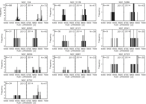
Observations were taken during 2013 and 2014 as part of an on-going programme at the Danish telescope that was implemented from April to September each year. Figure1 shows histograms of the number of observations per night per cluster. Data in the left-hand panel corresponds to 2013 and data in the right-hand panel, to 2014. As time at the telescope was limited, we tried to observe all clusters with the same rate as far as it was pos-sible by taking two observations each night. However, as it is shown in the histograms, this was not possible because of the weather conditions or because the telescope was used to monitor microlensing events carried out by the MINDSTEp consortium, as part of the programme to characterise exoplanets.

It is worth commenting that, depending on the magnitude level of the horizontal branch of each globular cluster, observa-tions with total exposure times between six to ten minutes were produced (see Sect.7). To do this the camera was continuously taking images (at the rate of ten images per second) for the total exposure time desired and then all the images obtained during that particular exposure time were stacked to produce a single observation. That is, a ten-minute exposure time observation is the result of stacking 6000 images that were taken continuously. The technique for image stacking is called “shift-and-add” and it is explained in Sect.2.3.2.

2.3. EMCCD data reduction

EMCCDs, also known as low-light-level charge-coupled devices (L3CCD; see e.g.Smith et al. 2008;Jerram et al. 2001), are con-ventional CCDs that are equipped with an extended serial gain register in which each electron produced during the exposure time has a probability of creating a second electron (avalanche multiplication) when it passes through the extended gain register. The process in which the second electrons are created is called impact ionisation.

To do bias, flat-field and tip-tilt corrections, the procedures and algorithms described inHarpsøe et al.(2012) were used.

2.3.1. Tip-tilt correction

As described inHarpsøe et al.(2012), the tip-tilt correction for a sample of bias and flat-field corrected images Ii(x, y) with respect to a reference imageR(x, y) is calculated by finding the global maximum ofPidefined by Eq. (1),

Pi(x, y)=|FFT−1[FFT(R)·FFT(Ii)]|, (1)

which is the correlation image (see Fourier cross-correlation theorem). The position of the maximum (xmax, ymax) is used to shift each of the images in the sampleIi(x, y) to the position of the stars in the reference image.

2.3.2. Image quality and stacking

The image quality is assessed by defining the quality index

qi=

Pi(xmax, ymax)

|(x−xmax,y−ymax)|<r

(x,y)(xmax,ymax)

Pi(x, y)

, (2)

which represents the ratio of the maximumPi(xmax, ymax) to the sum of thePi(x, y) values of the surrounding pixels. Once this index is calculated, images from a single observation are sorted from the one with the best quality (smallestqi) to the one with the worst quality (largestqi) and a ten-layer image frame is built by stacking images in the sequence: 1%, 2%, 5%, 10%, 20%, 50%, 90%, 98%, 99%, and 100%. This means that the first-layer frame has stacked the top 1% of the best quality images, the second-layer frame has stacked the next 1% of the best quality images, the third-layer frame has stacked the next 3%, the fourth has stacked the next 5%, and so on. In this study, we use the layers with the best full width at half maximun (FWHM) over all the frames to build the reference image for each globular cluster and we stack the ten layers of an observation into a single science image for the photometry (see alsoSkottfelt et al. 2015a).

2.4. Photometry

To extract the photometry in each of the images we used the DanDIA1_{pipeline (Bramich 2008;Bramich et al. 2013), which}

is based on difference image analysis (DIA).

As commented in Sect.2.3.2, for each EMCCD observation, we produced a ten-layer calibrated image cube where each of the images in the cube is sorted by quality. DanDIA builds a high S/N and high-resolution reference frame by selecting and combining the best quality images available in the cubes. This is done by detecting bright stars using DAOFIND (Stetson 1987)

1 _{DanDIA is built from the DanIDL library of IDL routines available}

Fig. 1.Histograms with the number of observations per night for each globular cluster studied in this work.Panels on the left: plotted data taken during 2013;panels on the right: data taken during 2014.

and employing these to align the images using the triangulation technique described inPál & Bakos(2006). Each of the refer-ence frames used in the analysis of each globular cluster can be found throughout the paper (e.g. Fig.6) and the mean PSF FWHM for each reference image is listed in Table3. Positions and reference fluxes (fref) in ADU/s for each star are calculated using the PSF photometry package “STARFINDER” (Diolaiti et al. 2000). The pipeline implements a low-order polynomial degree for the spatial variation of the PSF model (a quadratic polynomial degree was sufficient in our case).

Once the reference image is built, all of the science frames are registered with the reference image by once again using the Stetson (1987) and Pál & Bakos (2006) algorithms described before. Image subtraction then determines a spatially variable kernel, modelled as a discrete pixel array, that best matches the reference image to each science image. The photometric scale factor (p(t)) used to scale the reference frame to each image is calculated as part of the kernel model (Bramich et al. 2015). Difference images are created by subtracting the convolved ref-erence image from each science image. Finally, difference fluxes (fdiff(t)) in ADU/s for each star detected in the reference image are measured in each of the difference images by optimally scal-ing the PSF model for the star to the difference image. The light curve for each star is the total flux (ftot(t)) in ADU/s defined as

ftot(t)= fref+

fdiff(t)

p(t) · (3)

We transform this to instrumental magnitudesminsat each given timet:

mins(t)=17.5−2.5 log(ftot(t)). (4) A detailed description of the procedures and techniques em-ployed by the pipeline can be found inBramich et al.(2011).

For a conventional CCD, the noise model used by DanDIA is represented by the pixel variancesσ2

ki jof the imagekat the pixel positionsi, j

σ2 ki j=

σ2 0

F2

i j

+ Mki j

GFi j

, (5)

whereσ0is the CCD readout noise (ADU),Fi jis the master flat-field image,Gis the CCD gain (e−/ADU) andMki jis the image model. For an EMCCD, the noise model for a single exposure is different:

σ2 i j=

σ2 0

F2

i j

+ 2Mi j

Fi jGEMGPA

, (6)

whereGEM is the electron-multiplying gain (photons/e−) and

GPAis the Pre Amp gain (e−/ADU).

IfNexposures are combined by summation, then the noise model for the combined imageσ2

i j,combis given by Eq. (7): σ2

i j,comb=

Nσ2

0

F2_{i j} +

2Mi j,comb

Fi jGEMGPA

Table 1.Time-seriesIphotometry for all known and new variables in the field of view covered in each globular cluster.

Cluster Var Filter HJD Mstd Mins σm fref σref fdiff σdiff p

id (d) (mag) (mag) (mag) (ADU s−1_{) (ADU s}−1_{) (ADU s}−1_{) (ADU s}−1₎

NGC 104 PC1-V12 I 2 456 472.93210 15.846 6.777 0.014 24 971.015 9644.446 −30 350.989 1425.567 5.5131 NGC 104 PC1-V12 I 2 456 476.94 184 15.729 6.659 0.012 24 971.015 9644.446 −16 234.626 1138.337 4.9447

..

. ... ... ... ... ... ... ... ... ... ... ...

NGC 5139 V457 I 24 56 432.58154 15.735 6.649 0.007 20 096.379 684.928 +8409.333 673.724 4.6618 NGC 5139 V457 I 2456438.70588 15.832 6.746 0.005 20 096.379 684.928 −312.498 432.554 4.5021

..

. ... ... ... ... ... ... ... ... ... ... ...

NGC 5286 V37 I 2 456 445.53773 15.978 6.951 0.005 18 451.916 1202.455 −8631.145 385.937 4.6006 NGC 5286 V37 I 2 456 446.53053 15.744 6.717 0.003 18 451.916 1202.455 +9806.700 232.129 4.6341

..

. ... ... ... ... ... ... ... ... ... ... ...

Notes.The standardMstdand instrumentalMinsmagnitudes are listed in Cols. 5 and 6, respectively, corresponding to the cluster, variable star, filter,

and epoch of mid-exposure listed in Cols. 1−4, respectively. The uncertainty onMinsis listed in Col. 7, which also corresponds to the uncertainty

onMstd. For completeness, we also list the quantities fref,fdiff, andpfrom Eq. (3) in Cols. 8, 10, and 12, along with the uncertaintiesσrefandσdiff

in Cols. 9 and 11. This is an extract from the full table, which is available at the CDS.

Fig. 2.StandardImagnitude taken from the HST observations as a function of the instrumentali+zmagnitude. The red lines are the fits that best match the data and they are described by the equations in the titles of each plot. The correlation coefficient is 0.999 in all cases.

whereMi j,comb is the image model of the combined image (see alsoSkottfelt et al. 2015a).

In Table 1, we illustrate the format of the electronic table with all fluxes and photometric measurements as they are avail-able at the CDS.

2.5. Astrometry and finding chart

To fit an astrometric model for the reference images, celestial coordinates available in the ACS Globular Cluster Survey2_(see

Table 2. Convention used in the variable star classification of this work, based on the definitions of the general catalogue of variable stars (Samus et al. 2009a).

Type Id Point style Color

Pulsating variables

RR Lyrae (RRL) RR0 Filled circle Red RR01 Filled circle Blue RR1 Filled circle Green

Semi-regular SR Filled square Red

Long-period irregular L Filled square Purple SX Phoenicis SX Phe Filled triangle Cyan

Cataclysmic variables

In general DN, Novae Filled five pointed star Green Eclipsing variables

W Ursae Majoris-type EW Filled five pointed star Blue Unclassified variables

In general NC Filled square Yellow

Anderson et al. 2008) were uploaded for the field of the cluster throughGaia(Graphical Astronomy and Image Analysis Tool; Draper 2000). An (x,y) shift was applied to all of the uploaded positions until they matched the stars in the fields. Stars lying outside the field of view and those without a clear match were re-moved, and the (x, y) shift was refined by minimising the squared coordinate residuals. The number of stars used in the matching process ranged from 108 stars to 1034 stars, which guaranteed that the astrometric solutions that were applied to the reference images considered enough stars to cover the whole field. The ra-dial rms scatter obtained in the residuals was∼0.1 (∼1 pixel). The astrometrically calibrated reference images were used to produce a finding chart for each globular cluster on which we marked the positions and identifications of all variable stars stud-ied in this work. Finally, a table with the equatorial J2000 celes-tial coordinates of all variables for each globular cluster is given (see, e.g. Table4).

3. Photometric calibration

The photometric transformation of instrumental magnitudes to the standard system was accomplished using information available in the ACS Globular Cluster Survey, which provides calibrated magnitudes for selected stars in the fields of 50 glob-ular clusters extracted from images taken with theHubbleSpace Telescope (HST) instruments ACS and WFPC.

By matching the positions of the stars in the field of the HST images with those in our reference images, we obtained photo-metric transformations for our ten globular clusters, as shown in Fig.2. TheImagnitude obtained from the ACS (seeSirianni et al. 2005) is plotted versus the instrumentali+zmagnitude obtained in this study. The red lines are linear fits with slope unity yielding zero-points labelled in the title of each plot.Nis the number of stars used in the fit. The correlation coefficient was 0.999 in all cases. A transformation was derived for each globular cluster.

4. Colour magnitude diagrams

As our sample has data available for only one filter, we decided to build colour magnitude diagrams (CMD; see Fig.5) by us-ing the information available from the HST images at the ACS Globular Cluster Survey. The data used correspond to the V

andI photometry obtained inSirianni et al.(2005). The CMD

Fig. 3.Positions of the 157 known globular clusters in the Galaxy are plotted in the Galactic plane system. The 10 globular clusters studied in this work are labelled in red. Green corresponds to the globular clusters studied inSkottfelt et al.(2015a,2013).

Fig. 4.Root mean square (rms) magnitude deviation (top) andSB

statis-tic (bottom) versus the meanImagnitude for the 575 stars detected in the field of view of the reference image for NGC 104. Coloured points follow the convention adopted in Table2to identify the types of vari-ables found in the field of this globular cluster.

was useful in classifying the variable stars, especially those with poorly defined light curves such as long-period irregular variables and semi-regular variables, as well as corroborating cluster membership.

5. Variable star searches

During the reductions, the DanDIA pipeline produced a total of 12 541 light curves for stars in the cores of the ten globular clus-ters studied. We used three automatic (or semi-automatic) tech-niques to search for variable stars, as described in Sects.5.1−5.3.

5.1. Root mean square

Table 3.Some of the physical properties of the globular clusters studied in this work.

Section Cluster RA Dec D Dgc [Fe/H] E(B−V) VHB V−MV c ρ0 FW H M texp

NGC J2000 J2000 kpc kpc mag mag mag log(Lpc−3_{) arcsec s}

8.1 104 00:24:05.67 −72:04:52.6 4.5 7.4 −0.72 0.04 14.06 13.37 2.07 4.88 0.61 302.4 8.2 5139 13:26:47.24 −47:28:46.5 5.2 6.4 −1.53 0.12 14.51 13.94 1.31 3.15 0.38 312.0 8.3 5286 13:46:26.81 −51:22:27.3 11.7 8.9 −1.69 0.24 16.63 16.08 1.41 4.10 0.37 316.8 8.4 6093 16:17:02.41 −22:58:33.9 10.0 3.8 −1.75 0.18 16.10 15.56 1.68 4.79 0.45 302.4 8.5 6121 16:23:35.22 −26:31:32.7 2.2 5.9 −1.16 0.35 13.45 12.82 1.65 3.64 0.49 180.0 8.6 6541 18:08:02.36 −43:42:53.6 7.5 2.1 −1.81 0.14 15.35 14.82 1.86 4.65 0.56 340.8 8.7 6656 18:36:23.94 −23:54:17.1 3.2 4.9 −1.70 0.34 14.15 13.60 1.38 3.63 0.50 297.6 8.8 6681 18:43:12.76 −32:17:31.6 9.0 2.2 −1.62 0.07 15.55 14.99 2.50 5.82 0.49 312.0 8.9 6723 18:59:33.15 −36:37:56.1 8.7 2.6 −1.10 0.05 15.48 14.84 1.11 2.79 0.51 360.0 8.10 6752 19:10:52.11 −59:59:04.4 4.0 5.2 −1.54 0.04 13.70 13.13 2.50 5.04 0.59 198.0

Notes.Column 1 contains the section with the individual results for each globular cluster. Column 2 contains the name of the cluster as it is defined

in the New General Catalogue, Cols. 3 and 4 contain the celestial coordinates (right ascension and declination), Col. 5 shows the distance from the Sun, Col. 6 is the distance from the Galactic centre, Col. 7 shows metallicity, Col. 8 shows reddening, Col. 9 showsVmagnitude level of the horizontal branch, Col. 10 shosVdistance modulus, Col. 11 shows King-model central concentrationc=log(rt/rc), Col. 12 contains central

luminosity density log10(Lpc−3), Col. 13 contains the meanFWHM(arcsec) measured in the reference image and Col. 14 shows the exposure

time in the reference image.

To select possible variable stars, we fit a polynomial model to the rms values as a function of magnitude and flag all stars with rms values greater than three times the model. All difference im-ages obtained with DanDIA were blinked as well to corroborate the variation of the stars selected.

5.2. SBstatistic

A detailed discussion can be found about the benefits of using the SB statistic to detect variable stars (Figuera Jaimes et al. 2013) and RR Lyrae with Blazhko effect (Arellano Ferro et al. 2012). TheSBstatistic is defined as

SB=

1

N M

M

i=1

ri,1 σi,1 +

ri,2 σi,2 +

...+ ri,ki

σi,ki 2

, (8)

whereNis the number of data points for a given light curve and

Mis the number of groups formed of time-consecutive residuals of the same sign from a constant-brightness light curve model (e.g. mean or median). The residualsri,1tori,kicorrespond to the

ith group ofkitime-consecutive residuals of the same sign with corresponding uncertaintiesσi,1toσi,ki. TheSBstatistic is larger in value for light curves with long runs of consecutive data points above or below the mean, which is the case for variable stars with periods longer than the typical photometric cadence. Plots ofSB versus meanImagnitude are given for each globular cluster (see bottom Fig.4) and variable stars are plotted in colour.

To select variable stars, the same technique employed in5.1 was used, but in this case the threshold was shifted between 3−10 times the modelSBvalues, depending on the distribution of the data in each globular cluster. All stars selected were in-spected in the difference images in the same way as explained in Sect.5.1.

5.3. Stacked difference images

Based on the results obtained using the DanDIA pipeline, a stacked difference image was built for each globular cluster with the aim of detecting the difference fluxes that correspond to vari-able stars in the field of the reference image. The stacked image is the result of summing the absolute values of the difference

images divided by the respective pixel uncertainty

Si j =

k

|Dki j| σki j

, (9)

whereSi jis the stacked image,Dki jis thekth difference image, σki jis the pixel uncertainty associated with each imagekand the indexesiandjcorrespond to pixel positions.

All of the variable star candidates obtained by using the rms diagrams or theSBstatistic explained in Sects.5.1and5.2were inspected visually in the stacked images to confirm or refute their variability. Difference images were also blinked to finally cor-roborate the variation of the stars selected.

6. Variable star classification

All variable stars found were plotted in the colour–magnitude diagram for the corresponding globular cluster, to have a bet-ter understanding of the nature of their variation and their clus-ter membership. A period search of the light curve variations was undertaken by using the string method (Lafler & Kinman 1965) and by minimising theχ2in a Fourier analysis fit. To de-cide the classification of the variable stars, we used the conven-tions defined in the General Catalogue of Variable Stars (Samus et al. 2009a) and by considering their position in the colour– magnitude diagrams and the periods found.

In Table 2, the classification, corresponding symbols, and colours used in the plots throughout the paper are shown.

7. Globular clusters observed

Figure3shows the Galactic plane celestial coordinates (l,b) for the 157 globular clusters listed in (Harris 1996, 2010 edition). The ten globular clusters analysed in this work are plotted in red where six are in the southern hemisphere and four are in the northern hemisphere. Also plotted (in green) are the six globular clusters studied inSkottfelt et al.(2015a,2013).

The strategy to select and observe the clusters was the fol-lowing:

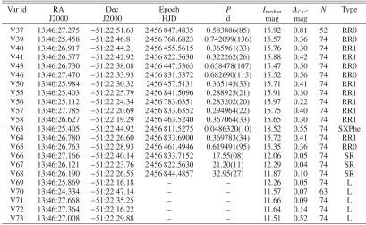
Table 4.NGC 104: ephemerides and main characteristics of the variable stars in the field of this globular cluster.

Var id RA Dec Epoch P Imedian Ai+z N Type

J2000 J2000 HJD d mag mag

PC1-V12 00:24:05.921 −72:04:45.20 – – 15.62 1.10 149 NC

WF2-V34 00:24:08.406 −72:04:35.91 – – 10.98 0.03 139 L

LW10 00:24:02.490 −72:05:07.45 – – 9.60 0.24 108 L

LW11 00:24:03.145 −72:04:50.60 2 456 920.7253 19.37(8) 10.18 0.08 141 SR

LW12 00:24:03.982 −72:05:10.06 – – 9.57 0.09 41 L

EM1 00:24:03.065 −72:04:55.02 2 456 491.9380 20.28(9) 10.26 0.05 145 SR EM2 00:24:06.269 −72:04:45.36 2 456 530.7986 31.50(22) 9.98 0.08 140 SR EM3 00:24:08.310 −72:04:50.69 2 456 847.9667 33.41(24) 10.07 0.05 134 SR EM4 00:24:07.203 −72:04:46.45 2 456 498.9086 68.07(102) 13.89 0.14 149 SR

EM5 00:24:05.087 −72:04:54.38 – – 10.34 0.06 145 L

EM6 00:24:02.733 −72:05:02.80 – – 10.60 0.07 147 L

EM7 00:24:07.885 −72:05:02.00 – – – – 146 NC

Notes.Column 1 contains the id assigned to the variable star, Cols. 2 and 3 correspond to the right ascension and declination (J2000), Col. 4 shows

the epoch used, Col. 5 shows the period, Col. 6 contains median of the data, Col. 7 shows the peak-to-peak amplitude in the light curve, Col. 8 contains the number of epochs and Col. 9 shows the classification of the variable. The numbers in parentheses indicate the uncertainty on the last decimal place of the period.

Table 5.NGC 5139: ephemerides and main characteristics of the variable stars in the field of this globular cluster.

Var id RA Dec Epoch P Imedian Ai+z N Type

J2000 J2000 HJD d mag mag

V457 13:26:46.246 −47:28:44.81 – – 15.82 0.15 78 NC V458 13:26:46.103 −47:28:57.05 – – 10.21 0.04 78 L V459 13:26:46.313 −47:28:40.33 – – 10.98 0.06 78 L

Notes.Columns are the same as in Table4.

(2) We focused on the concentration of stars in the central re-gion of the clusters. As reference, we used the central lumi-nosity densityρ0(Lpc−3) listed in (Harris 1996, 2010

edi-tion). The entire sample, which is available in the catalogue, has log(ρ0) from∼0 to∼6. To explore the potential of the EMCCD and the shift-and-add technique for photometry, a sample with different levels ofρ0were chosen from a very dense cluster NGC 6752 (log(ρ0) = 5.04) to a less dense cluster NGC 6723 (log(ρ0) = 2.79) and some intermedi-ate levels as NGC 5139 (log(ρ0) = 3.15) and NGC 5286 (log(ρ0)=4.10).

(3) A bibliography review revealed how many variable stars are known from previous work. To do this, we used the informa-tion available for each globular cluster in the Catalogue of Variable Stars in Galactic Globular Clusters (Clement et al. 2001) and the ADS to do the bibliography review up-to-now. (4) Exploration of known colour–magnitude diagrams. As most of the variable stars that are globular cluster members have a particular position in these diagrams, we focused our at-tention on globular clusters with a high concentration of stars, for example at the top of the red giant branch (for semi-regular variables), the instability strip of the horizon-tal branch (for RR Lyrae), and the blue straggler region (for SX Phoenicis). To do this we used the colour information available in the ACS to build colour–magnitude diagrams for each globular cluster. Additionally, we also used the Galactic globular clusters database3.

5) The exposure time to be used for a single EMCCD obser-vation for each globular cluster was chosen based on the

3 _{http://gclusters.altervista.org/}

Vmagnitude of the horizontal branch. We selected exposure times as follows:

6 min forVHB<14 mag,

8 min for 14 mag<VHB<17 mag, 10 min forVHB>17 mag.

We chose the ten globular clusters presented in this work. Some of their most relevant physical properties are detailed in Table3.

8. Results

8.1. NGC 104 / C0021-723 / 47 Tucanae

The globular cluster was discovered by Nicholas Louis de Lacaille in 17514. The cluster is in the constellation of Tucana at a distance of 4.5 kpc from the Sun and 7.4 kpc from the Galactic centre. It has a metallicity of [Fe/H]=−0.72 dex and a distance modulus of (m−M)V =13.37 mag. The magnitude of its hori-zontal branch isVHB=14.06 mag.

In Fig. 4, the root mean square magnitude deviation (top) andSBstatistic (bottom) are plotted versus the meanI magni-tude for a total of 575 light curves that were extracted in this analysis. The coloured points correspond to the variable stars studied in this work compared to the stars where no variation is found (normal black points).

8.1.1. Known variables

This globular cluster has approximately 300 known variable sources in the Catalogue of Variable Stars in Galactic Globular Clusters (version of summer 2007; Clement et al. 2001), which

Fig. 5.Colour magnitude diagram for the globular cluster NGC 104 built withVandImagnitudes available in the ACS globular cluster sur-vey extracted from HST images. The variable stars are plotted in colour following the convention adopted in Table2.

include long-period irregular variables, SX Phoenicis, RR Lyrae, and binary systems. Most were found byAlbrow et al.(2001), Weldrake et al.(2004), andLebzelter & Wood(2005). There are also 20 millisecond pulsars listed in the literature for this cluster (Freire et al. 2001). However, no visual counterparts have been found at their positions.

In the field of view covered by the reference image (Fig.6), there are 49 previously known variables. However, for this clus-ter we were only able to detect stars brighclus-ter thanI =16.1 mag (see rms in Fig.4). As a result, five known variable stars, which were brighter than this limit, were detected. These stars are la-belled in the literature as PC1-V12, WF2-V34, LW10, LW11, and LW12. Our light curves for these variables can be found in Fig.7.

PC1-V12: this star was discovered byAlbrow et al.(2001)

and classified as a blue straggler star (BSS) with an average mag-nitude ofV =16.076 mag. No period was reported in this case and it was not possible to find a period for this star in the present work.

WF2-V34: the variability of this star was discovered by

Albrow et al.(2001) and was classified as a semi-regular variable with a period ofP=5.5 d. However, using this period it was not possible to produce a good phased light curve and it was not possible to find another period for this star. Based on this, we classified this star as a long-period irregular variable.

LW10-LW12: these three stars were discovered byLebzelter

& Wood(2005). Their positions in the colour–magnitude dia-gram (Fig. 5) confirm their cluster membership. Lebzelter & Wood(2005) classified them as long-period irregular variables and suggested periods for these stars to be LW10: 110 d or 221 d, LW11: 36.0 d, and LW12 : 61 d or 116 d. However, LW10 and LW12 are clearly irregular variables (see our Figs. 7 and 1 fromLebzelter & Wood 2005). For LW11 we found a period of 19.37 d and we classify it as semi-regular.

8.1.2. New variables

After extracting and analysing all possible variable sources in the field of our images, a total of seven new variables (EM1-EM7) were found of which four are semi-regular variables, two are long-period irregular variables and one is unclassified.

Fig. 6.Finding chart for the globular cluster NGC 104. The image used corresponds to the reference image constructed during the reduction. All known variables and new discoveries are labelled. Image size is

∼41 ×41 arcsec2_.

For this cluster, the nomenclature employed for most of the variable stars discovered in previous works does not correspond to the typical numbering system (e.g. V1, V2, V3, ... , Vn). For example, variables discovered byLebzelter & Wood(2005) and Weldrake et al.(2004) are numbered using their initials LW and W, respectively;Albrow et al.(2001) used a PC or WF nomen-clature that makes reference to the instrument employed during the observations. As a result, we did not find it practical to assign the typical numbering system to the new variable stars discov-ered in this work and we decided to use as reference the EMCCD camera used in the observations. That is, new variables are num-bered as EM1-EM7.

EM1-EM4: these variable stars are placed at the top of the

colour magnitude diagram (Fig.5). Their light curve shape, am-plitudes and periods found suggest that these stars are semi-regular variables. Periods found for these variables are listed in Table4. The star EM1 is not over the red giant branch in Fig.5 but instead is more towards the asymptotic giant branch, appear-ing at the top on the left. Finally the star EM4 is located at the bottom part of the red giant branch just below the starting point of the horizontal branch.

EM5-EM6: these stars have amplitudes of ∼0.06 and

0.07 mag, respectively. They are located at the top of the red giant branch. We were not able to determine a proper period for these stars. Consequently, we classified them as long-period ir-regular variables.

Fig. 7.NGC 104: light curves of the known and new variables discovered in this globular cluster. Red triangles correspond to the data obtained during the year 2013 and blue circles correspond to the data obtained during the year 2014. For EM7, we plot the quantity fdiff(t)/p(t) since a

reference flux is not available.

8.2. NGC 5139 / C1323-472/ Omega Centauri

This globular cluster was discovered by Edmond Halley in 16775_{. The cluster is in the constellation of Centaurus at 5.2 kpc}

from the Sun and 6.4 kpc from the Galactic centre. It has a metallicity of [Fe/H] = −1.53 dex, a distance modulus of (m−M)V = 13.94 mag and the level of the horizontal branch is atVHB=14.51 mag.

8.2.1. Known variables

In the Catalogue of Variable Stars in Galactic Globular Clusters (Clement et al. 2001), there are approximately 400 variable stars for this globular cluster. Most of these variables were discovered by Bailey (1902), Kaluzny et al. (2004) and Weldrake et al. (2007). All of the known variables are outside the field of view of our reference image. Most recently,Navarrete et al. (2015) made an updated analysis of the variables in this cluster, but the variables in their study are also located outside the field of view of our reference image.

8.2.2. New variables

We found three new variables in this globular cluster. Two are long-period irregular variables and one is unclassified.

The new variable stars are plotted in the rms diagram andSB statistic (see Fig.8). Based on the position of the stars in Figs.8 and9, there is no evidence of RR Lyrae in the field covered by this work or in the inspection of the difference images obtained in the reductions.

5 _{http://messier.seds.org/xtra/ngc/n5139.html}

V457: this variable star has an amplitude of∼0.15 mag with a median magnitudeI=15.82 mag. It lies on the RGB and we were unable to find a period.

V458, V459: theses two stars are at the top of the red giant

branch in Fig.9and have amplitudes of∼0.04 and∼0.06 mag, respectively. No periods were found in this work. V459 is on the red side of the main red giant branch. We classify them as long-period irregular variables.

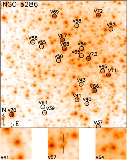
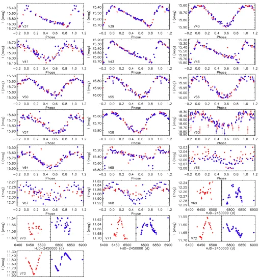
8.3. NGC 5286 / C1343-511 / Caldwell 84

This globular cluster was discovered by James Dunlop in 1827 (O’Meara 2002). It is in the constellation of Centaurus at 11.7 kpc from the Sun and 8.9 kpc from the Galactic centre. It has a metallicity of [Fe/H]=−1.69 dex, a distance modulus of (m−M)V =16.08 mag, and the magnitude level of the horizontal branch is atVHB=16.63 mag.

In Fig.12, the rms diagram and the SBstatistic are shown for the sample of 1903 stars that were analysed in this globular cluster. Most of them have 74 epochs. All variable stars studied in this work are plotted using the colour classification given in Table2.

8.3.1. Known variables

Table 6.NGC 5286: ephemerides and main characteristics of the variable stars in the field of this globular cluster.

Var id RA Dec Epoch P Imedian Ai+z N Type

J2000 J2000 HJD d mag mag

V37 13:46:27.275 −51:22:51.63 2 456 847.4835 0.583886(85) 15.92 0.81 52 RR0 V39 13:46:25.458 −51:22:46.81 2 456 768.6823 0.742099(136) 15.57 0.36 74 RR0 V40 13:46:26.917 −51:22:44.21 2 456 455.5615 0.365961(33) 15.76 0.30 74 RR1 V41 13:46:26.577 −51:22:42.92 2 456 822.5630 0.322262(26) 15.88 0.42 74 RR1 V43 13:46:26.730 −51:22:38.08 2 456 447.5363 0.658478(107) 15.47 0.50 74 RR0 V46 13:46:27.470 −51:22:33.93 2 456 831.5372 0.682690(115) 15.52 0.56 74 RR0 V50 13:46:25.984 −51:22:30.32 2456 457.5131 0.365145(33) 15.71 0.41 74 RR1 V55 13:46:25.403 −51:22:25.79 2 456 841.5096 0.288925(21) 15.91 0.30 74 RR1 V56 13:46:25.112 −51:22:24.34 2 456 783.6351 0.283202(20) 15.97 0.22 74 RR1 V57 13:46:27.785 −51:22:20.69 2 456 833.6352 0.294964(22) 15.75 0.40 74 RR1 V58 13:46:26.627 −51:22:19.29 2 456 463.5240 0.367064(33) 15.65 0.30 74 RR1 V63 13:46:25.405 −51:22:44.92 2 456 811.5275 0.0486320(10) 18.52 0.55 74 SXPhe V64 13:46:26.780 −51:22:26.60 2 456 833.6900 0.369783(34) 15.72 0.41 74 RR1 V65 13:46:26.763 −51:22:28.93 2 456 461.4946 0.619491(95) 15.35 0.36 74 RR0 V66 13:46:27.166 −51:22:40.14 2 456 833.7152 17.55(08) 12.06 0.05 74 SR V67 13:46:26.121 −51:22:23.76 2 456 822.5630 21.20(11) 12.29 0.04 74 SR V68 13:46:26.190 −51:22:26.55 2 456 844.4857 32.95(27) 11.87 0.10 74 SR

V69 13:46:25.869 −51:22:16.18 – – 12.26 0.05 74 L

V70 13:46:24.334 −51:22:47.14 – – 11.57 0.07 63 L

V71 13:46:27.668 −51:22:35.25 – – 11.66 0.09 74 L

V72 13:46:27.364 −51:22:16.22 – – 11.64 0.14 74 L

V73 13:46:27.008 −51:22:29.88 – – 11.51 0.52 74 L

Notes.Columns are the same as in Table4.

Table 7.NGC 6093: ephemerides and main characteristics of the variable stars in the field of this globular cluster.

Var id RA Dec Epoch P Imedian Ai+z N Type

J2000 J2000 HJD d mag mag

V10 16:17:01.163 −22:58:34.57 2 456 805.5870 0.614154(92) 14.25 0.29 52 RR0 V17 16:17:02.864 −22:58:32.55 2 456 831.5535 0.415081(42) 15.31 0.31 62 RR1 V19 16:17:02.107 −22:58:29.10 2 456 844.5144 0.596064(87) 15.28 0.54 62 RR0 V20 16:17:03.263 −22:58:37.49 2 456 831.5535 0.745207(136) 15.31 0.46 62 RR0

V34 16:17:02.820 −22:58:33.80 – – 16.44 0.36 62 CV(Nova)

V35 16:17:03.313 −22:58:33.15 – – 11.40 0.09 62 L

V36 16:17:03.145 −22:58:41.92 – – 11.50 0.12 62 L

V37 16:17:02.320 −22:58:30.48 – – 11.51 0.09 62 L

V38 16:17:03.263 −22:58:34.96 – – 11.70 0.04 62 L

V39 16:17:02.201 −22:58:34.49 – – 11.75 0.07 62 L

V40 16:17:03.042 −22:58:25.72 – – 12.36 0.13 62 L

Notes.Columns are the same as in Table4.

discovered byZorotovic et al.(2010) using DIA on imaging data from a one-week observing run.

The celestial coordinates given in Table 1 ofZorotovic et al. (2010) do not match the positions of the known variable stars in the field of our images. We therefore used the finding chart given in their Fig. 1 to do a visual matching of the variables. As pointed out in the Catalogue of Variable Stars in Galactic Globular Clusters (Clement et al. 2001), there is a difference in the position of the variables studied byZorotovic et al.(2010) with respect to the position of the variables in Samus et al. (2009b), which is∼6 arcsec in declination and1 arcsec in right ascension. This difference is corroborated by the position of the variables in our reference image. Celestial coordinates of the po-sitions we used are given in Table6.

Our extended observational baseline has allowed us to greatly improve the periods of the variables discovered by Zorotovic et al.(2010). Our period estimates are listed in Table6

and have typical errors of 0.00002−0.00010 d. We confirm the variable star classifications made byZorotovic et al.(2010). We note that V41 is a strong blend with a brighter star that is only just resolved in our high-resolution reference image.

8.3.2. New variables

In this globular cluster we found 11 previously unknown variables where five are long-period irregular variables, three are semi-regular variables, two are RR Lyrae, and one is an SX Phoenicis.

Fig. 8.Root mean square (rms) magnitude deviation (top) andSB

statis-tic (bottom) versus the meanImagnitude for the 2616 stars detected in the field of view of the reference image for NGC 5139. Coloured points follow the convention adopted in Table2to identify the types of vari-ables found in the field of this globular cluster.

Fig. 9.Colour magnitude diagram of the globular cluster NGC 5139 built withV andI magnitudes available in the ACS globular cluster survey extracted from HST images. The variable stars are plotted in colour following the convention adopted in Table2.

V64: this star is an RR Lyrae pulsating in the first over-tone (RR1) with a period of 0.369783 d and an amplitude of 0.41 mag. In Fig.14, it is clear that V64 is very close to a bright star (6.808 pixels or 0.613 arcsec). This could be the reason why this variable was not discovered before and makes a good exam-ple of the benefits of using the EMCCD cameras and the shift-and-add technique along with DIA.

V65: this star is another RR Lyrae which is pulsating in the fundamental mode (RR0) with a period of 0.619491 d and an amplitude of∼0.36 mag.

V66-V68: these stars are semi-regular variables. As can be

seen in Fig.13, they are at the top of the red giant branch. They have amplitudes that range between 0.04 to 0.10 mag. They have periods between∼17 to 33 d. Ephemerides for these stars can be found in Table6.

V69-V73: these five stars are also positioned at the top of

the red giant branch with amplitudes of 0.05 to 0.52 mag. It was not possible to find periods for these stars in this work.

Fig. 10. Finding chart for the globular cluster NGC 5139. The im-age used corresponds to the reference imim-age constructed during the reduction. The new variables discovered are labelled. Image size is

∼41 ×41 arcsec2_.

Consequently, they were classified as long-period irregular vari-ables.

In Fig.16the amplitude-period diagram for the RR Lyrae stars studied in this cluster is shown. The filled lines correspond to the Oosterhofftype I (OoI) and the dashed lines correspond to the Oosterhofftype II (OoII) models defined byKunder et al. (2013). All RR0 variables (with the exception of V65) fall into the model for OoII type while the RR1 stars scatter around both models. In this diagram the RR0 stars suggest an OoII type clas-sification for NGC 5286, which is in agreement with the study done byZorotovic et al.(2010) where they found that their re-search pointed to an OoII status as well.

8.4. NGC 6093 / C1614-228 / M 80

This globular cluster was discovered by Charles Messier in 17816_{. This cluster is in the constellation of Scorpius at 10.0 kpc}

from the Sun and 3.8 kpc from the Galactic centre. Its has a metallicity of [Fe/H] = −1.75 dex, a distance modulus of (m−M)V =15.56 mag and the position of its horizontal branch is atV=16.10 mag.

A total of 1220 light curves were extracted in the field cov-ered by the reference image for the globular cluster NGC 6093. Most of the stars have 58 epochs in their light curves and vari-able stars studied in this work are plotted with colour in the rms andSBdiagrams shown in Fig.17.

8.4.1. Known variables

This globular cluster has 34 known variable sources in the Catalogue of Variable Stars in Galactic Globular Clusters (Clement et al. 2001). Only seven are in the field of view cov-ered by these observations. There is no visual detection of V11 in our images (discovered byShara et al. 2005, and classified as

Fig. 11.NGC 5139: light curves of the three new variables discovered in this globular cluster. Symbols are the same as in Fig.7.

Table 8.NGC 6121: ephemerides and main characteristics of one variable star in the field of this globular cluster.

Var id RA Dec Epoch P Imedian Ai+z N Type

J2000 J2000 HJD d mag mag

V21 16:23:35.903 −26:31:33.68 2 456 477.5041 0.472008(56) 12.55 0.92 64 RR0

Notes.Columns are the same as in Table4.

Fig. 12. Root mean square (rms) magnitude deviation (top) and SB

statistic (bottom) versus the mean Imagnitude for the 1903 stars de-tected in the field of view of the reference image for NGC 5286. Coloured points follow the convention adopted in Table2to identify the types of variables found in the field of this globular cluster.

Fig. 13.Colour magnitude diagram for the globular cluster NGC 5286 built withV andI magnitudes available in the ACS globular cluster survey extracted from HST images. The variable stars are plotted in colour following the convention adopted in Table2.

Fig. 14.Finding chart for the globular cluster NGC 5286. The image used corresponds to the reference image constructed during the reduc-tion. All known variables and new discoveries are labelled. Image size is∼41×41 arcsec2_{. The image stamps are of size∼4.6×4.6 arcsec}2_.

a possible U Geminorum-type cataclysmic variable). This is to be expected since it has a U mean magnitude of 19.5 mag. The star V33 was discovered byDieball et al.(2010) in an ultravi-olet survey using theHubbleSpace Telescope. They reported a UV magnitude for this target of about 19.8 mag. Again, it was not possible to obtain a light curve for this faint target.

Fig. 15.NGC 5286: light curves of the known and new variables discovered in this globular cluster. Symbols are the same as in Fig.7.

by Kopacki (2013) for the four RR Lyrae variables since we observed them using a time baseline of over one year, whereas Kopacki(2013) analysed observations spanning only one week.

V34: this is the Nova discovered by Arthur von Auwers at Koenigsberg Observatory on May 21, 1860 (Luther 1860). As pointed out in the Catalogue of Variable Stars in Galactic Globular Clusters (Clement et al. 2001), an account of its dis-covery was given bySawyer(1938) in which a maximum visual

apparent magnitude of 6.8 mag was reported using the data taken by von Auwers and Luther. Another review can also be found inWehlau et al.(1990). However, no observations of the Nova in outburst have been made until the present study. During our 2013 observing campaign, we caught an outburst of amplitude

Fig. 16.Amplitude-period diagram for the RR Lyrae stars in the globu-lar cluster NGC 5286.

Fig. 17. Root mean square (rms) magnitude deviation (top) and SB

statistic (bottom) versus the mean Imagnitude for the 1220 stars de-tected in the field of view of the reference image for NGC 6093. Coloured points follow the convention adopted in Table2to identify the types of variables found in the field of this globular cluster.

Dieball et al. (2010) in their ultraviolet survey assigned the label CX01 to an X-ray source that was found to be associated with the position of the Nova at the coordinates RA(J2000) = 16:17:02.817 and Dec(J2000) = −22:58:33.92. These coordinates match with the position of the outburst found in this work and details are given in Table7.

The position in the colour magnitude diagram shown in Fig.18suggests that this system is a cluster member. It is lo-cated at the bottom part of the red giant branch. Its position is plotted with a green five pointed star.

As the Nova with its outburst has shown variability, we have assigned the label V34 to this object.

8.4.2. New variables

A total of six new variables were found in this work. All of them are long-period irregular variables.

V35-V40: these stars are long-period irregular variables.

They are located at the top of the red giant branch (see Fig.18). Their amplitudes go from∼0.04 to 0.13 mag. The star V40 is the one placed on the blue side of the red giant branch. We did

Fig. 18.Colour magnitude diagram for the globular cluster NGC 6093 built withV and I magnitudes available in the ACS globular cluster survey extracted from HST images. The variable stars are plotted in colour following the convention adopted in Table2.

Fig. 19.Finding chart for the globular cluster NGC 6093. The image used corresponds to the reference image constructed during the reduc-tion. All known variables and new discoveries are labelled. Image size is∼41×41 arcsec2_.

not find any kind of regular periodicity in the variation of these stars.

8.5. NGC 6121 / C1620-264 / M4

This globular cluster was discovered by Philippe Loys de Chéseaux in 17467_{. This cluster is in the constellation of}

Scorpius at a distance of 2.2 kpc from the Sun and 5.9 kpc from the Galactic centre. It has a metallicity of [Fe/H]=−1.16 dex and a distance modulus of (m−M)V =12.82 mag. Its horizontal branch level is atVHB=13.45 mag.

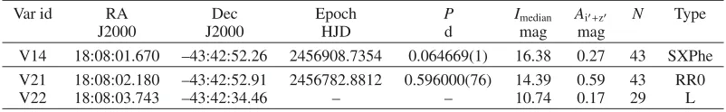
Table 9.NGC 6541: Ephemerides and main characteristics of the variable stars in the field of this globular cluster. Columns are the same as in Table4.

Var id RA Dec Epoch P Imedian Ai+z N Type

J2000 J2000 HJD d mag mag

V14 18:08:01.670 –43:42:52.26 2456908.7354 0.064669(1) 16.38 0.27 43 SXPhe V21 18:08:02.180 –43:42:52.91 2456782.8812 0.596000(76) 14.39 0.59 43 RR0

V22 18:08:03.743 –43:42:34.46 – – 10.74 0.17 29 L

Table 10.NGC 6656: ephemerides and main characteristics of the variable stars in the field of this globular cluster.

Var id RA Dec Epoch P Imedian Ai+z N Type

J2000 J2000 HJD d mag mag

V35 18:36:24.051 −23:54:29.53 2456472.8818 141(5) 9.43 0.13 19 SR PK-06 18:36:25.228 −23:54:37.44 2456789.8239 0.140851(4) 17.08 0.65 51 EW

CV1 18:36:24.696 −23:54:35.60 2456877.6355 – 17.87 3.28 51 CV(DN)

Notes.Columns are the same as in Table4.

Table 11.NGC 6681: ephemerides and main characteristics of one variable star in the field of this globular cluster.

Var id RA Dec Epoch P Imedian Ai+z N Type

J2000 J2000 HJD d mag mag

V6 18:43:12.015 −32:17:29.70 2 456 814.8334 0.341644(25) 15.09 0.23 50 RR1

Notes.Columns are the same as in Table4.

Fig. 20.NGC 6093: light curves of the known and new variables discovered in this globular cluster. Symbols are the same as in Fig.7.

This globular cluster has approximately 100 known variables in the Catalogue of Variable Stars in Galactic Globular Clusters (Clement et al. 2001) and only three are in the field of view of the reference image; namely V21, V81, and V101. Furthermore, only V21 is bright enough to be detected. The light curve for this RR0 star is shown in Fig.22. The known periodP= 0.4720 d produces a very well phased light curve and is in agreement with the periodP=0.472008 d found in the analysis of this star.

No new variable stars were found in the field covered by the reference image for this globular cluster.

8.6. NGC 6541 / C1804-437

This globular cluster was discovered by N. Cacciatore in 18268_.

It is in the constellation of Corona Australis at 7.5 kpc from

Fig. 21.Finding chart for the globular cluster NGC 6121. The image used corresponds to the reference image constructed during the reduc-tion. The only known variable in the field is labelled. Image size is

∼41×41 arcsec2_.

Fig. 22.NGC 6121: light curve of the variable V21 in this globular clus-ter. Symbols are the same as in Fig.7.

the Sun and 2.1 kpc from the Galactic centre. The cluster has a metallicity of [Fe/H] = −1.81 dex, a distance modulus of (m−M)V = 14.82 mag and the level of the horizontal branch is at VHB = 15.35 mag. A total of 843 light curves were ex-tracted in this globular cluster. Most of them have 42 epochs. rms diagram andSBstatistic are shown in Fig.23.

8.6.1. Known variables

This globular cluster has 20 known variables. Four of them are in the field of view of our reference image: V12, V14, V15, and V17.Fiorentino et al.(2014) discovered and classified these stars as SX Phoenicis in their study carried out using observations with the HST. We were only able to recover V14 in our data around 2 arcsec in declination from the reported position for this star inFiorentino et al.(2014). We did not detect variability at the positions given for V12, V15, and V17 or in their surrounding areas, probably because the stars are too faint to be detected in our reference image. A reference image with higher S/N might be needed in future studies of this globular cluster and longer exposure times for each observation.

V14: for this star we refined the period estimate to 0.064669 d from the previously listed value of 0.0649 d in Fiorentino et al.(2014).

Fig. 23. Root mean square (rms) magnitude deviation (top) and SB

statistic (bottom) versus the meanImagnitude for the 843 stars detected in the field of view of the reference image for NGC 6541. Coloured points follow the convention adopted in Table2to identify the types of variables found in the field of this globular cluster.

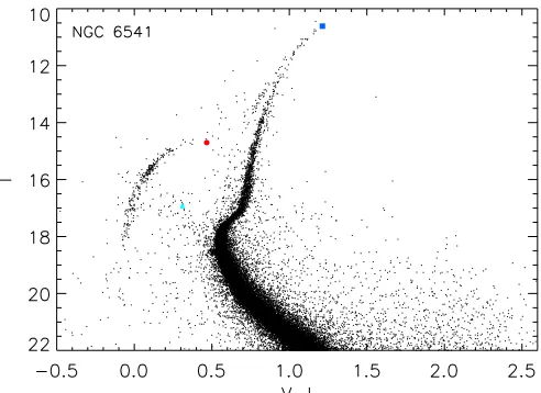
Fig. 24.Colour magnitude diagram for the globular cluster NGC 6541 built withV and I magnitudes available in the ACS globular cluster survey extracted from HST images. The variable stars are plotted in colour following the convention adopted in Table2.

8.6.2. New variables

A total of two new variable stars were found in this globular cluster: one RR Lyrae and one long-period irregular variable.

V21: this star is a RR Lyrae pulsating in the fundamental mode. In the colour–magnitude diagram (Fig.24) for this cluster it falls exactly in the instability strip of the horizontal branch. It is next to a brighter star (∼1.039 arcsec) and this may be why it was not discovered before.

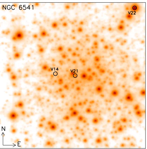
Fig. 25.Finding chart for the globular cluster NGC 6541. The image used corresponds to the reference image constructed during the reduc-tion. All known variables and new discoveries are labelled. Image size is∼41 ×41 arcsec2_.

8.7. NGC 6656 / C1833-239 / M 22

This globular cluster was discovered by Abraham Ihle in 16659_.

It is in the constellation of Sagittarius at 3.2 kpc from the Sun and 4.9 kpc from the Galactic centre. The cluster has a metallicity of [Fe/H] = −1.70 dex, a distance modulus of (m−M)V = 13.60 mag and the horizontal branch level is at

VHB=14.15 mag.

8.7.1. Known variables

There are approximately 100 variable sources known for this globular cluster. Only four of these are inside the field of view of the reference image (V35, PK-06, PK-08, and CV1). PK-08 is too faint for us to extract a light curve.

V35:this star is the brightest star in our field of view and it is classified as a semi-regular variable. The star is at the top of the red giant branch in the colour–magnitude diagram shown in Fig.29.Sahay et al.(2014) found a period of∼56 d. However, we found a period of 141±5 d.

PK-06: this star is classified as an EW eclipsing variable.

It was discovered by Pietrukowicz & Kaluzny (2003) and it is their star M22_06. They found a periodP = 0.239431 d. However, it does not produce a good phased light curve in our data. In the analysis of this variable, we found a period of

P=0.140851 d which produces a better phased light curve (see Fig.28). However, our phased light curve is still not as clear as that ofPietrukowicz & Kaluzny(2003).

CV1:the variability of this star was first detected bySahu et al.(2001) as a suspected microlensing event, but it was not untilAnderson et al. (2003) that it was classified as a dwarf nova outburst. The analysis of our light curve for this source shows that it undergoes an outburst of ∼3 mag around HJD

∼2 456 877, which decays over ∼20d. It is in agreement with

9 _{http://messier.seds.org/m/m022.html}

previous studies. Anderson et al. (2003) found that an earlier outburst lasted∼20−26d with an amplitude of∼3 mag peaking atI ≈ 15 mag.Alonso-Garcia et al.(2015) also observed the 2014 outburst seen in our data and reported a Ks-band brighten-ing of 1 mag. In Fig.28, we have plotted the light curve for this star.

Our search for new variable sources in this cluster did not yield any.

8.8. NGC 6681 / C1840-323 / M70

This globular cluster was discovered by Charles Messier in 178010. The globular cluster is in the constellation of Sagittarius at 9.0 kpc from the Sun and 2.2 kpc from the Galactic centre. It has a metallicity of [Fe/H]=−1.62 dex, a distance modulus of (m−M)V =14.99 mag and the horizontal branch level is at

VHB=15.55 mag.

There are a total of 1315 light curves available for this cluster to be analysed. Most of them have 50 epochs. The rms andSB diagrams can be found in Fig.30. Variable stars studied in this work are plotted in colour.

8.8.1. Known variables

This globular cluster has only five known variables, none of which are in the field of view of our reference image.

Kadla et al. (1996) reported several RR Lyrae candidates based on the position of the stars in the instability strip of the horizontal branch but none of them matched the position of the only variable star found in the field of view covered by our refer-ence image, which is the new variable V6 explained in the next section.

8.8.2. New variables

One new RR Lyrae was discovered in this globular cluster.

V6: this star has an amplitude of 0.23 mag and a period of

P = 0.341644 d. The star is placed just at the instability strip of the horizontal branch (see Fig.31). It is clearly a previously unknown RR Lyrae of type RR1. The light curve for this variable is shown in Fig.33.

8.9. NGC 6723 / C1856-367

This globular cluster was discovered by James Dunlop in 182611_.

It is in the constellation of Sagittarius at a distance of 8.7 kpc from the Sun and 2.6 kpc from the Galactic centre. It has a metallicity of [Fe/H] = −1.10 dex, a distance modulus of (m−M)V = 14.84 mag and the horizontal branch level is at

VHB=15.48 mag.

In Fig.34, the rms andSBstatistic diagrams for 1258 stars in the globular cluster NGC 6723 are shown. Most of the light curves have 56 epochs. Variable stars analysed in this work are plotted in colour following the convention adopted in Table2.

8.9.1. Known variables

This globular cluster has 47 known variables stars in the Catalogue of Variable Stars in Galactic Globular Clusters

10 _{http://messier.seds.org/m/m070.html}

Fig. 26.NGC 6541: light curves of the known and new variables discovered in this globular cluster. Symbols are the same as in Fig.7.

Table 12.NGC 6723: ephemerides and main characteristics of the variable stars in the field of this globular cluster.

Var id RA Dec Epoch P Imedian Ai+z N Type

J2000 J2000 HJD d mag mag

V8 18:59:34.678 −36:37:42.33 2 456 908.5573 0.480278(49) 15.08 0.71 16 RR0 V34 18:59:33.189 −36:37:58.04 2 456 435.8962 0.531414(60) 14.85 0.84 56 RR0 V35 18:59:32.963 −36:38:01.46 2 456 524.8178 0.606451(78) 14.80 0.32 56 RR0 V44 18:59:32.347 −36:37:51.96 2 456 454.9399 0.440075(41) 15.08 0.93 56 RR0

Notes.Columns are the same as in Table4.

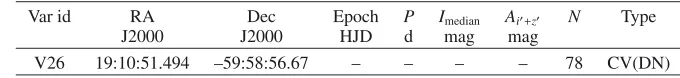
Table 13.NGC 6752: ephemerides and main characteristics of one variable star in the field of this globular cluster.

Var id RA Dec Epoch P Imedian Ai+z N Type

J2000 J2000 HJD d mag mag

V26 19:10:51.494 –59:58:56.67 – – – – 78 CV(DN)

Notes.Columns are the same as in Table4.

Fig. 27.Finding chart for the globular cluster NGC 6656. The image used corresponds to the reference image constructed during the reduc-tion. All known variables and new discoveries are labelled. Image size is∼41×41 arcsec2_.

(Clement et al. 2001). 43 are classified as RR Lyrae, two as semi-regular variables, one as a T Tauri star that does not seem to be a cluster member and one as a SX Phoenicis. Four of the known RR Lyrae are in the field of our reference frame (V8, V34, V35 and V44). They are RR0 pulsating stars. The star V8 was discov-ered byBailey(1902) and although it is close to the reference

image border, it was possible to obtain 16 data points. The stars V34, V35, and V44 were discovered byLee et al.(2014). In the colour magnitude diagram for this globular cluster (see Fig.36), these variables are placed just in the instability strip of the hor-izontal branch. Light curves for these variables are shown in Fig.38.

The four RR Lyrae in the field of our images are plotted in the period-amplitude diagram shown in Fig.35. It is possible to see that, even though V34 and V35 have the Blazhko effect, all of them are following the model of fundamental mode pul-sating stars for Oosterhofftype I, which is consistent with the Oosterhoff classification for this cluster (see Lee et al. 2014, Kovacs et al. 1986, and references therein).

The periods that we derive for the 4 RR Lyrae stars are per-fectly consistent with those derived byLee et al. (2014) using a 10-year baseline. Furthermore, the Blazhko effect in V34 and V35 is also evident in our light curves.

No new variable stars were found in the field covered by the reference image for this globular cluster.

8.10. NGC 6752 / C1906-600 / C93

This globular cluster was discovered by James Dunlop in 182612_.

It is in the constellation of Pavo with a distance of 4.0 kpc from the Sun and 5.2 kpc from the Galactic centre. It has a metallicity of [Fe/H] = −1.54 dex, a distance modulus of (m−M)V = 13.13 mag and the level of its horizontal branch is atVHB=13.70 mag.

Fig. 28.NGC 6656: light curves of the known variables found in this globular cluster. Symbols are the same as in Fig.7.

Fig. 29.Colour magnitude diagram for the globular cluster NGC 6656 built withV andI magnitudes available in the ACS globular cluster survey extracted from HST images. The variable stars are plotted in colour following the convention adopted in Table2.

Fig. 30. Root mean square (rms) magnitude deviation (top) and SB

statistic (bottom) versus the mean Imagnitude for the 1315 stars de-tected in the field of view of the reference image for NGC 6681. The coloured point follows the convention adopted in Table2to identify the types of variables found in the field of this globular cluster.

8.10.1. Known variables

There are 32 known variable sources in this globular cluster which are listed in the Catalogue of Variable Stars in Galactic Globular Clusters (Clement et al. 2001). Six of them are in the field of view of our reference image. Three are millisecond pul-sars (PSRB, PSRD, and PSRE) discovered byD’Amico et al. (2001, 2002). We could not find an optical counterpart in our reference image. Three more are Dwarf Novae (V25, V26, V27) discovered byThomson et al.(2012) of which V26 is the only object in which we could detect variability.

V26:this star is classified as a dwarf nova. A finding chart for V26 is already available inThomson et al.(2012). It was not

Fig. 31.Colour magnitude diagram for the globular cluster NGC 6681 built withV and I magnitudes available in the ACS globular cluster survey extracted from HST images. One variable star is plotted in colour following the convention adopted in Table2.

Fig. 32.Finding chart for the globular cluster NGC 6681. The image used corresponds to the reference image constructed during the reduc-tion. All known variables and new discoveries are labelled. Image size is∼41×41 arcsec2_.

Fig. 33.NGC 6681: light curve of the new variable discovered in this globular cluster. Symbols are the same as in Fig.7.

Fig. 34. Root mean square (rms) magnitude deviation (top) and SB

statistic (bottom) versus the mean Imagnitude for the 1258 stars de-tected in the field of view of the reference image for NGC 6723. Coloured points follow the convention adopted in Table2to identify the types of variables found in the field of this globular cluster.

Fig. 35.Period-amplitude diagram for the globular cluster NGC 6723. The previously known RR Lyrae are plotted.

the outburst started around HJD 2 456 840 with a maximum at HJD ∼ 2 456 858.8532 and lasted∼80 d.

We did not find any evidence in our data for new variable stars in this globular cluster.

9. Conclusions

This study shows how the effects of the atmospheric turbulence can be minimized on images taken with ground-based telescopes by using EMCCDs and the “shift-and-add” technique. With this

Fig. 36.Colour magnitude diagram for the globular cluster NGC 6723 built withV and I magnitudes available in the ACS globular cluster survey extracted from HST images. The variable stars are plotted in colour following the convention adopted in Table2.

Fig. 37.Finding chart for the globular cluster NGC 6723. The image used corresponds to the reference image constructed during the reduc-tion. All known variables and new discoveries are labelled. Image size is∼41×41 arcsec2_.

technique was also possible to avoid saturated stars in the field of the globular clusters observed which allowed the discovery of variable stars in the brightest zone of the colour−magnitude diagram such as the top of the red giant branch. The new dis-coveries are good examples that globular cluster systems still need further studies and are not as well understood as we have thought. A summary of the results obtained in this work are the following:

1. The central regions of ten globular clusters were studied. 2. The benefits of using EMCCDs and the shift-and-add

tech-nique were shown.