Quantum correlations in the one dimensional driven dissipative XY model

Quantum correlations in the one-dimensional driven dissipative

X Y

model

Chaitanya Joshi,1,*_{Felix Nissen,}2_{and Jonathan Keeling}1

1_{Scottish Universities Physics Alliance, School of Physics and Astronomy, University of St Andrews, St Andrews KY16 9SS, United Kingdom} 2_{London Centre for Nanotechnology, University College London, 17-19 Gordon St, London WC1H 0AH, United Kingdom}

(Received 3 October 2013; published 20 December 2013)

We study the nonequilibrium steady state (NESS) of a driven dissipative one-dimensional system near a critical point, and explore how the quantum correlations compare to the known critical behavior in the ground state. The model we study corresponds to a cavity array driven parametrically at a two photon resonance, equivalent in a rotating frame to a transverse field anisotropicXY model [C.-E. Bardyn and A. Imamo˘glu,Phys. Rev. Lett.

109,253606(2012)]. Depending on the sign of transverse field, the steady state of the open system can be either related to the ground state or to the maximum energy state. In both cases, many properties of the entanglement are similar to the ground state, although no critical behavior occurs. As one varies from the Ising limit to the isotropic

XYlimit, entanglement range grows. The isotropic limit of the NESS is, however, singular, with simultaneously diverging range and vanishing magnitude of entanglement. This singular limiting behavior is quite distinct from the ground state behavior; it can, however, be understood analytically within spin-wave theory.

DOI:10.1103/PhysRevA.88.063835 PACS number(s): 42.50.Dv,03.65.Ud,03.75.Gg,75.10.Pq I. INTRODUCTION

A central feature of critical behavior in any non-mean-field phase transition is the existence of a diverging correlation length [1,2]. Such divergences explain why universal theories, controlled only by symmetries of the problem, apply in the vicinity of a critical point. They also lead to scaling behavior [2] of correlation functions. More recently, it has been noted that measures of specificallyquantumcorrelation, e.g., entanglement [3], also show scaling behavior [4–7]. Entanglement is one of the characteristic traits of quantum mechanics [3] and is of practical significance as it captures quantum correlations which can be a resource for quantum cryptography, quantum teleportation, and dense coding [8]. Despite the diverging correlation length at critical points, entanglement generally has a finite range [4,5,7]; critical scaling is instead seen in the magnitude of the entanglement.

In a dissipative system, coupling to an external environ-ment [9] leads to dephasing, and consequent degradation of quantum correlations, ultimately reducing the system to a classical description [10,11]. Nonetheless, in a coherently driven dissipative system, i.e., pumped by an external coherent drive, nontrivial steady states can be found [12–29]. In an extended interacting driven dissipative system, such as an array of coupled nonlinear cavities as discussed below, this enables nonlocal quantum correlations to exist in the nonequilibrium steady state. Such systems allow one to study quantum correlations out of equilibrium, and to study whether dissipation has particular significance for distinctively quantum correlations such as entanglement.

The aim of this paper is to explore the range and scaling of quantum correlations in the nonequilibrium steady state (NESS) near to a critical point of the corresponding equi-librium system. A natural system in which to address such questions is an array of coupled cavities [30–34]. Such systems allow for tunable coupling and nonlinearity, and inevitably have dissipation, as light escapes from the cavities. Recently

*_{[email protected]}

Bardyn and Imamo˘glu [35] have shown that such systems can in certain limits map to dissipative spin chain models, as explained below. Their proposed configuration allows tuning of both the anisotropy of the spin-spin coupling, and of a transverse field. We study the nonequilibrium steady state, i.e., the long-time behavior, in the presence of dissipation. Within this scenario, we determine the dependence of quantum correlations on both of these parameters, exploring the range from the transverse field Ising model to the transverse field XY model.

The transverse field Ising model is a paradigmatic example of quantum critical behavior [1], and so the scaling of entangle-ment in the equilibrium Ising model (or anisotropicXYmodel) was one of the first examples studied [4–6]. As noted above, while the magnitude of entanglement shows critical scaling, the range over which nonzero entanglement exists does not [4,5]. This finite range behavior persists for all models in the Ising universality class [5,36,37]. Following these early studies, there have been many subsequent explorations of critical entanglement, including the spin-boson system [38] which can be viewed as a phase transition of a dissipative quantum system. For a review, see Ref. [7].

matrix product operators (MPO) [50–52]. This allows one to efficiently time evolve the density matrix equations of motion for one-dimensional (1D) open systems, and thus find the nonequilibrium steady state.

The remainder of this paper is organized as follows. SectionIIreviews the basis of our calculations. In particular, Secs. II A and II B introduce the effective Hamiltonian we study and its coupling to an external environment; Sec. II C reviews the measures of quantum correlations we calculate; and Sec. II D outlines the MPO method we use to find the steady state. Section III then presents the results of our numerical calculation. After reviewing the nature of the steady state in Sec.III A, and comparing these results to the mean-field theory of our model in Sec. III B, Secs. III C– III E discuss the dependence of quantum correlations on each of the model parameters in turn. Finally, Sec. IV discusses analytic calculations which can reproduce the behavior seen for weak driving. In Sec.Vwe summarize our findings.

II. DRIVEN-DISSIPATIVE MODEL AND OBSERVABLES A. Effective Hamiltonian

We consider a coupled cavity array realization of the transverse field anisotropic XY model, as introduced in Ref. [35]. For completeness, we briefly summarize the nature of such a model here. As illustrated in Fig.1the model consists of a 1D array of optical cavities, supporting photon modes, described by bosonic operators cj with hopping amplitude J between the cavities so that H=hj−J

j[cj†cj₊1+ H.c.]. The on-site Hamiltonian hj =ωcc†jcj +U c†jc†jcjcj incorporates an optical nonlinearity U. Physically this can be induced by coupling each cavity to a saturable optical absorber [25,30,33].

In addition to these elements, which would lead to a Bose-Hubbard model [53], we include a two-photon driving term as proposed in Ref. [35]. Specifically, we consider a drivecos(2ωpt) near two-photon resonance, i.e.,ωp ωc, and we work in the limit of strong optical nonlinearity. In this limit, the problem simplifies, as one may truncate each site to occupations 0 or 1. Furthermore, this implies that the two-photon pump is only resonant for the creation of pairs of photons on adjacent cavities. When restricted to the 0,1 occupation subspace, one may replace each cavity mode with a spin 1/2, i.e., replace bosonic operators by Pauli matrices (c_j,c†_j)→(σ_j−,σ_j+). Here σ_j±=(σ_jx±iσ_jy)/2 in terms of regular Pauli matrices. In this notation, the Hamiltonian

J J J J

κ κ κ κ κ

Ω Ω Ω Ω

FIG. 1. (Color online) Cartoon illustrating coupled cavity array with hoppingJ, two-cavity pumping, and loss rateκ.

becomes ˆ

H₀=

j ωc

2 σ z j −J

j

(σ_j+σ_j−₊₁+σ_j−σ_j+₊₁)

−

j

(σ_j+σ_j+₊₁e−2iωpt+_σ−

j σj−+1e2

iωpt_{). (1)}

The explicit time dependence appearing here can be removed by a transformation to a rotating frame. In such a frame the Hamiltonian is given by

ˆ

H = −J

j

gσ_jz+(σ_j+σ_j−₊₁+σ_j+₊₁σ_j−)

+(σ_j+σ_j+₊₁+σ_j−₊₁σ_j−), (2)

where we have introduced dimensionless parameters g= (ωp−ωc)/2J and=/J. This can also be written in the canonical form of the Ising model [54]:

ˆ

H = −J

j

gσ_jz+1+ 2 σ

x jσ

x j+1+

1− 2 σ

y jσ

y j+1

. (3)

The parameterdescribes the anisotropy of the interaction: =0 corresponds to the isotropic XY model, and =1 to the Ising model. For 0<||1 the Hamiltonian is in the Ising universality class. In the ground state, changing the transverse fieldgwill induce a quantum phase transition [1] at|g| =1, between a phase withσx =0 for|g|<1, and a phase with vanishingσxfor|g|>1.

B. Dissipation

In addition to the terms described so far, each cavity is also assumed to couple to a continuum of radiation modes describing irreversible loss into the environment [9]. At optical cavity and pump frequencies, one may eliminate such modes via the Born-Markov approximation [9,55], producing the master equation

d

dtρ= −i[ ˆH ,ρ]+κ

j

[2σ_j−ρσ_j+−σ_j+σ_j−ρ−ρσ_j+σ_j−].

(4)

The dissipation described in Eq. (4) corresponds to indepen-dent incoherent loss from each cavity. In the spin language, this corresponds to a process that flips the spin from up to down. Such dissipation corresponds to a zero-temperature bath; this is appropriate when considering optical frequency systems as the characteristic energy scales are much larger than temperature. In the following we introduce the dimensionless ˜κ =κ/J, and consider the steady state of the system as a function of the parameters (g,,κ˜). In the remainder of the paper all energies are thus given in units ofJ.

not satisfy detailed balance due to the “extra” time dependence induced by the pump frequency [57]. The crossover between these limits as one variesωc,ωp while keepinggconstant is an interesting question for future work.

C. Measures of quantum correlations

To quantify the quantum correlations between different sites requires some care, since a given pair of sites will in general be entangled both with other sites and with the external environment. As such, it is important to use a measure of the quantum correlation between a specific pair of sites. The measure of pairwise entanglement we will use will be negativityN defined as

N =max

0, 4

i

|λi| −1 , (5)

where λi are the eigenvalues of the partially transposed two-qubit density matrixρTB

AB[3], whereTBindicates transpose for system B. According to the Peres-Horodecki criterion [58,59] a (mixed) state of a bipartite system is separable if the negativity is zero. For any separable state, the density matrix would remain positive under a partial transpose. In an entangled state a partial transpose may produce a nonpositive density matrix [60]. The negativity as defined in Eq. (5) is a measure of whether the partial transpose produces negative eigenvalues. A nonzero value of negativity serves both as a necessary and sufficient condition for the inseparability of a general two-qubit state [58,59].

For pure states entanglement is a sufficient measure of quantum correlations and quantifies the ability of a state to act as a resource for quantum computational speedup [61]. For mixed states separability (vanishing entanglement) does not in general imply classicality [62–64]—computational speedup for mixed state quantum computing can occur without entanglement [65]. Such speedup has been attributed to the presence of nonzero quantum discord [62–66]Ddefined [64] as follows: Consider a bipartite systemABin a stateρ, and a local measurement performed on subsystemB with its result ignored. Such a measurement will cause a disturbance of subsystemAfor almost all states. There is, however, a class of states that is unchanged by such a measurement. For such statesχ ∈, known as “classical-quantum” states, one may writeχ =_ipiρAi⊗ |iB Bi|, wherepiis a probability distribution,ρAiis the marginal density matrix ofA, and the states|iBform an orthonormal set. Geometric discordDis the distance between the stateρand the closest classical-quantum state χ ∈. Explicitly, for an arbitrary mixed stateρ of a d⊗d quantum system it is D(ρ)= _d−d₁minχ∈||ρ−χ||2, where ||M|| =√_im2

i is the Hilbert-Schmidt norm of the operatorMwith eigenvaluesmi.

In the specific case of two-level systems (qubits), a closed form forDexists [64,67]. Writing the state of two qubits as

ρ =1 4

3

i,j=0

Rijσi⊗σj, R=

1 yT x t

, (6)

where σ_j0,1,2,3 = {1j,σjx,σ y j,σ

z

j}, and R is given in block structure above, one may then construct the 3×3 matrix

S=(1/4)(xxT _+ttT_{) from which}

D=2 Tr[S]−2λ_max(S), (7) whereλmax(S) is the largest eigenvalue of the matrixS.

D. Matrix product state evolution

As noted above, to find the nonequilibrium steady state, we time evolve Eq. (4) using a matrix product operator approach [50–52]. We here briefly summarize the method used in our calculation. Further details of our specific implementation can be found in Ref. [68].

Our problem requires time evolving the density matrix of a chain ofN two-level systems. This density matrix may be written in the form

ρ =

{i1,i2,...,iN}

ci1,i2,...,iN

N

j=1 σij

j (8)

withσ_j0,1,2,3 as given earlier forming a basis for the density matrix on each site. The central point of the MPO approach is to write the coefficientsci1,i2,...,iN in terms of matrices

[j]ij

and vectorsλ[j]_{as follows:}

ci1,i2,...,iN =

{αj}

[1]i1

1,α1λ

[1] α1

[2]i2 α1,α2· · ·

[j₋1]ij−1 αj−2,αj−1λ

[j−1] αj−1

[j]ij

αj−1,αj· · ·

×[N−1]iN−1 αN−2,αN−1λ

[N−1] αN−1

[N]iN

αN−1,1.

The matrix[j]ij_{, corresponding to basis componenti}

j on site j, is aχj−1×χj matrix, and λ[j] is a set ofχj coefficients associated with the bond between sitej and sitej+1. Here χj is the (integer) bond dimension of the matrix associated with bond j. If all χj =1, then one has entirely separable density matrix, i.e., ρ=ρj, equivalent to a mean-field approximation. If χj are sufficiently large, any state can be written in the above form—the required size for our two-level-system density matrix is χj =min(4j,4N−j). To efficiently simulate such a system we restrict χj < χmax. For a fixed χmax, the size of computation scales linearly with chain length. Despite this, the representation is able to accurately describe the full quantum dynamics in many problems.

To time evolve the state, we follow the algorithm described in Refs. [40,51]. The master equation may be written in a superoperator form, with the density matrix as a vector ρ → |ρ, so that∂t|ρ =M|ρ. The superoperatorMcan be decomposed asM=_jM_j,jpair₊₁, with the one-site operations split between the appropriate pair operators. Evolution by a time step δt corresponds to propagating the coefficients [j]ij_,λ[j] _{under the operator exp(M}pair

j,j₊1δt). This is done by converting the MPO representation for a given pair of sites into its explicit form, evolving the pair, and then performing a singular value decomposition (SVD) [3] to return the final form to MPO representation. The rank χj after such an update will generally have increased, but can be restored to χj χmaxby keeping only the largestχmaxsingular values in the SVD.

N

g

− −

FIG. 2. (Color online) NegativityN vs transverse fieldg, com-paring MPO numerical solution forχmax=20 (blue, solid) to exact diagonalization (red, dashed) for a four-site Ising model. Parameters (in units ofJ):=1, ˜κ=0.5.

eModdδt/2eMevenδteModdδt/2+O(δt3). SinceModdinvolves a sum of pair operations which each mutually commute, all the updates inModd_{can be performed in parallel. The same applies} toMeven_.

To demonstrate the accuracy of our implementation [68], Fig.2shows a comparison between exact diagonalization of the four-site master equation and the open system MPO code with χmax=20 showing close agreement. These results, as all results in our paper, are calculated for a chain with open boundary conditions. For longer chains, comparison with exact solutions is not feasible so we instead check for convergence of numerical results with matrix rankχmax. Efficient simulation depends on whether convergence is achieved for sufficiently small values of the matrix rank χmax. If correlation lengths diverge, such as at critical points, strong long-range corre-lations exist. In such cases convergence would only occur at large χmax and and evolution becomes computationally expensive. In our system, we will see that the dissipation ˜κ suppresses such long-range correlations; for small values of

˜

κ the computational cost would increase, particularly near the equilibrium critical points|g| =1. It is important also to note that in this paper we are only concerned with convergence of the steady-state properties. If one is also interested in the short-time dynamics, the required matrix rank may be much larger [69], due to transient correlations arising before dissipation has time to act. In addition to convergence with matrix rank, we also find and check that properties near the middle of the chain converge with increasing chain length.

III. SCALING OF QUANTUM CORRELATIONS IN NONEQUILIBRIUM STEADY STATES A. Nature of the nonequilibrium steady state

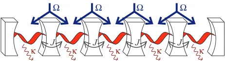
Before discussing the quantum correlations in the nonequi-librium steady state of Eq. (4), we first discuss the nature of the steady state itself. The dissipation term on its own would drive the system to a state with all spins pointing down. In the following we denote this state as the trivial empty state. In general (unless =0), this trivial state is not an eigenstate of the Hamiltonian so is not the steady state. An observable that gives a clear indication of the nature of the steady state is

−

g

−

−

−

σ

_σ

l l l l

σx _σx l

l

− −

− −

− −

−

(a)

(b)

(c)

FIG. 3. (Color online) Panel (a) showing spin-spin correlations

σx

jσjx+l as a function of transverse field. The different lines

correspond to different separations. Panel (b) showing decay of spin-spin correlationsσx

jσjx+las a function of separationlbetween

the spin sites. Both panels plotted for the Ising limit (=1). It is clearly seen that the NESS exhibit FM and AFM ordering for negative and positive values of transverse field (g= ±1). Inset [panel (c)] shows short-range incommensurate order for lower values of transverse field (g= ±0.1). The axes in the inset are the same as in the main plot. Other parameters (in units ofJ): ˜κ=0.5 and MPO calculation performed forN=40 site chain, withχmax=20.

the correlation functionσx jσ

x

j+l. This is plotted in Fig.3for =1, for sites near the center of the chain, hence avoiding edge effects.

As is clear from Fig.3, in the NESS, the x components of spin show (short-range) ferromagnetic order for transverse fields aroundg −1 and antiferromagnetic order for fields around g1. In comparison, in the ground state of the Ising model there are ferromagnetic correlations for |g|< 1, regardless of the sign of g. As will be proven below, there is a direct relation between the NESS for positive and negative g, corresponding to aπ rotation around the z axis on every second lattice site. This duality implies that if (short-range) ferromagnetic correlations are seen for a giveng, antiferromagnetic correlations will exist forg→ −g. As well as this formal duality, we will also discuss next a more intuitive picture for the different behaviors at positive and negativeg, a picture substantiated by analytic results of mean-field analysis given in Sec.III B.

collective dynamics generally correspond to stationary points of the closed-system dynamics. Such stationary points will correspond to extrema of the energy. The ferromagnetic correlations seen forg <0 clearly reflect the properties of the ground state, including a peak in correlations nearg= −1, where the ground state undergoes a quantum phase transition. In contrast, for large positivegthe ground state is incompatible with the dissipation. However, the maximum energy state, which is also a stationary point of the dynamics is compatible with the dissipation. The behavior of the correlations seen in Fig.3suggests that forg <0, the attractor of the dynamics is related to the ground state, while for g >0 the attractor is instead related to the state of maximum energy. Similar behavior has been seen in the dynamics of the Dicke model, where duality under change of sign of cavity-pump detuning leads to an inverted normal state [70].

The proof of the duality under change of the sign of g follows by considering transformations of the density matrix that relate its steady state forg to that for−g. We consider dividing the chain into sublattices of odd and even sites. The switch from ferro- to antiferromagnetic order is equivalent to the statement that correlations between sites on different (the same) sublattices are odd (even) functions of the field g. Two dualities are required to show this. First, duality under Hˆ → −Hˆ, ρ→ρ∗. This follows from taking the complex (notHermitian) conjugate of the equation of motion. Since both ˆH and all the loss terms are real, this complex conjugation means that ˆH → −Hˆ is equivalent toρ→ρ∗. The second duality concerns rotation around the z axis on one sublattice,ρ→Rˆ_oddρRˆ_odd, where ˆR_odd=_j=1,3,5...σ_jz; this has the effect of modifying Eq. (3) by changing the sign of the intersite couplings; this is equivalent to the combinationH → −H,g→ −g. Combining this duality with complex conjugation, one finds that interchangingg→ −g alone is equivalent toρ→Rˆ_oddρ∗Rˆ_odd. This transformation swaps the sign of correlations between the two sublattices as required. The dualities involved make clear the role of the inversionH → −Hin relating the steady states forg→ −g, corroborating the statement that the g >0 steady state is related to the maximum energy state.

As can be seen in Fig. 3(c), for small values of g, correlations become small, and vanish asg=0. In the smallg regime these small short-range correlations are neither strictly ferromagnetic nor antiferromagnetic, but instead show an incommensurate ordering. Such behavior occurs in a regime where the mean-field theory would predict the trivial state. (Note that in other models, mean-field theory can also predict incommensurate orderings [27].) As expected the spin-spin correlation functions always respect the sublattice dualities as discussed above.

The appearance of the trivial state as an attractor atg→0, cannot be simply related to minimum or maximum energy states as in the earlier discussion. Note also that the above dualities do not explain why the same-sublattice correlators, which are even functions ofg, should vanish atg=0. The state at g=0 can nonetheless be directly understood: at g=0, =1, the effective magnetic field seen by any site points purely in thexdirection, and so the evolution combines precession around thexaxis with decay. Consequently, thex component of all spins vanishes at this point. The correlators

σ_jyσ_jy_+l(not shown) do not generally vanish atg=0, but still show the odd–even symmetry discussed above. For <1 the

σx jσ

x

j+ldo not vanish atg=0 either; this is discussed further in Sec.III D.

B. Comparison with the mean-field theory

To further understand the differences between the NESS and the ground state, we next discuss the mean-field prediction for the NESS. While mean-field theory incorrectly predicts long-range order in low dimensions, the nature of the order predicted is reflected by the full MPO numerics. Within mean-field theory it is possible to give closed-form expressions for the phase boundary, and for the nature of the order anticipated for given values ofg,,κ. This provides further intuition for the differences between the NESS and the ground state.

In mean-field theory, the full density matrix is approximated as a product state (i.e., equivalent to restrictingχ_max=1 in an MPO simulation). The equations of motion then reduce to the following set of nonlinear Bloch equations:

d dt

ˆ

σ_jx= −κ˜σˆ_jx+2gσˆ_jy−(1−)σˆ_jzσˆ_jy₋₁+σˆ_jy₊₁,

d dt

ˆ

σ_jy= −κ˜σˆ_jy−2gσˆ_jx+(1+)σˆ_jzσˆ_jx₋₁+σˆ_jx₊₁,

d dt

ˆ

σ_jz= −2 ˜κσˆ_jz+1−(1+)σˆ_jyσˆ_jx₋₁+σˆ_jx₊₁

+(1−)σˆ_jxσˆ_jy₋₁+σˆ_jy₊₁. (9) One may either directly time evolve these equations to determine steady states, or attempt to analytically solve these equations in cases where the spatial dependence is relatively simple. Below we first present the analytical approach, and then discuss direct numerical evolution.

It is clear from Eq. (9) that the trivial stateσˆx j = σˆ

y j = 0,σˆ_jz = −1 is always a fixed point, i.e., a steady state. This trivial state does not break the Z2 symmetry of Eq. (4) and so can also be referred to as a paramagnetic state [27]. While such a steady state always exists, this state need not always be stable to small fluctuations. To test linear stability, one may linearize the equations of motion around the steady state, and consider plane-wave fluctuations of the form

⎛ ⎝σˆ

x j

σˆ_jy

σˆ_jz

⎞ ⎠_{= −}

⎛ ⎝00

1

⎞

⎠₊

k

⎛ ⎝xykk

zk

⎞

⎠e−iνkt−ij k_.

The equations of motion then yield a secular equation for the frequenciesνk, with solutions

νk= −iκ˜±2

g2_{+2gcos(k)+(1−}2_{) cos}2_{(k) (10)}

and νk= −2iκ˜. The steady state is stable to such a plane-wave fluctuation k if [νk]<0, meaning such fluctuations exponentially decay.

Δ

−

−

˜

κ

g

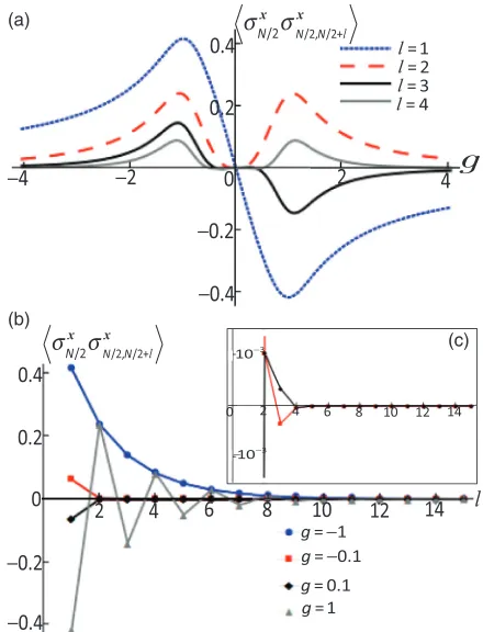
FIG. 4. (Color online) Mean-field phase diagram for the nonequilibrium steady state of Eq. (4) as a function of dimensionless parametersg,,κ˜.

one can write a simple expression for the phase boundary, ˜

κ =21−(g±1)2_{, indicating that for small enough ˜κ the} normal state is unstable near tog= ±1.

In addition to the trivial state one may consider the FM ansatz σˆx

j =X,σˆ y

j =Y,σˆ z

j =Z, or AFM ansatz

σˆ_jx =(−1)jX,σˆ_jy =(−1)jY,σˆ_jz =Z, and then find X,Y,Z by substituting these forms into Eq. (9) and solving the resulting cubic equation. One finds that for negative g, there is a nontrivial FM solution (X,Y=0), which exists only when the trivial state is unstable. (When the trivial state is stable, the cubic equation only has one real root corresponding toX=Y =0, Z= −1.) Forg >0 the same statements apply to the AFM ansatz. Whenever these nontrivial solutions exist they can be shown to be stable.

This analysis predicts a simple phase diagram, corroborated by direct numerical time evolution of Eq. (9). There are three phases: trivial, FM, and AFM. The boundaries between these are given by the surfacesνπ =0, ν0=0 withνk from Eq. (10). This phase diagram is shown in Fig.4as a function of parameters g,,κ˜. It is clear that for a fixed ˜κ and with decreasing value of, the range of the transverse field strength g over which the FM and AFM exist decreases. As→0, for finite κ, the trivial state always occurs regardless of the valueg.

To compare the predictions of mean-field theory and the full numerics, Fig.5compares their predictions for the correlation function σˆ_jxσˆ_jx₊₁ as a function of transverse field strength g. In the trivial state, mean-field theory (MFT) predicts this correlation to vanish, while in the ordered states it predicts

±X2_{, for the FM (AFM) states, respectively. As can be} seen, MFT does predict the kind of order that is seen, but predicts sharp phase boundaries that are not seen in the full numerics.

As noted above, direct time evolution of Eqs. (9) corrob-orate the above phase diagram. However, the steady state found does depend on the initial conditions used. Specifically, considering small periodic perturbations around the trivial state and time evolving Eq. (9) yields the AFM, trivial, and FM states exactly as discussed above. In contrast, if time

−

g

−

σx _σx

−

FIG. 5. (Color online) Spin-spin correlationsσx

jσjx+1as a func-tion of transverse field strength g. Parameters (in units of J):

=1,κ˜ =0.5 and MPO calculation performed for theN=40 site chain, withχmax=20.

evolved from a random initial configuration, domains of FM or AFM can exist, separated by defect sites (domain walls). The dynamics of such domain walls becomes frozen within the mean-field numerics. The absence of long-range order seen in the full MPO numerics can be considered as the effect of a superposition of many different configurations of domain walls.

C. Correlations vs transverse field in the Ising limit We now turn to the properties of quantum correlations at=1 (the Ising model). For comparison, we summarize here the ground state properties, as studied in [4–6]. In the Ising model entanglement is short ranged: Only nearest- and next-nearest-neighboring spins are entangled. The magnitude of the nearest-neighbor entanglement, however, shows critical scaling. At the critical point |g| =1 Ref. [4] showed that dC/dg (where C is concurrence, another measure of entan-glement) scaled as a power of the system size. Consequently, the peak value of C(g) actually occurs for |g|>1, rather than at the critical point. In the ground state, nearest-neighbor entanglement only vanished atg→0,|g| → ∞[4]. Quantum discord for the same model was studied in Ref. [36]. Discord is not restricted to nearest neighbors, and is peaked near

|g| =1.

Figure6shows the evolution of quantum correlations (neg-ativity [71] and geometric quantum discord) with transverse fieldgin the nonequilibrium steady state at=1,κ˜ =0.5. In addition, the integrated susceptibility Sxx

int =

jσ x i σ

x j (static spin structure factor) is shown. This correlation function both serves as an example of a correlation function that does not require specifically quantum correlations, and also as a function which would diverge (as a power law of system size) at the ground state critical point—such a divergence reflects the appearance of quasi-long-range order in the spin-spin correlator. The asymmetry of this correlation function seen in Fig. 6(c) reflects the switch from ferromagnetic to antiferromagnetic order.

g

−

−

N

l

=

g

D

l=

l=

l=

l=

−

−

= = =

g

Sxx

int

−

− −

(a)

(b)

(c)

FIG. 6. (Color online) Evolution of quantum correlations with transverse field g in the Ising limit. Panel (a) shows negativity

N, and panel (b) geometric quantum discord D. In addition the integrated susceptibility Sxx

int =

jσ x

iσjx is shown in (c); at the

equilibrium critical point this would show a power-law divergence with system size. Note that only one line is shown in panel (a) because entanglement vanishes beyond nearest neighbors at

=1. Parameters as in Fig.3.

discord extends to greater separations, Fig. 6(b). Negativity also peaks at a value |g|>1. These features exist for both signs of g; this is because the entanglement measures are not affected by the sublattice sign changes induced by the duality discussed above. As discussed in Ref. [72], two-mode squeezing is a sufficient condition for pairwise entanglement. We have confirmed that in the range ofgfor which bipartite en-tanglement vanishes, the two-mode spin squeezing parameter is identically zero.

In contrast to the ground state, there is, however, no critical behavior: The entanglement is an analytic function of g with no singular behavior at |g| =1. Similarly, the integrated susceptibility does not diverge with increasing

system size but instead saturates. This reflects exponential spatial decay of correlations, i.e., a finite correlation length, as anticipated due to the dissipation. The absence of critical behavior and the presence of only short-range correlations suggests the NESS of this 1D system does not undergo any phase transition. Such a result is to be expected, since any finite temperature leads to short-range order for a 1D system with short-ranged interactions. Although we consider dissipation due to an empty (i.e., zero-temperature) bath, we consider a nonequilibrium situation. As has been discussed elsewhere (see, e.g., [23,24]), this leads to a nonzero low-energy effective temperature.

Also in contrast to the ground state behavior, for small|g| entanglement vanishes entirely. The nature of this disappear-ance, i.e., the sharp threshold seen in Fig. 6(a), is a general feature of entanglement in a dissipative system [73]—finite amounts of dissipation can make a state become separable. Discord, however, remains nonzero between nearest neighbors atg=0.

D. Correlations vs anisotropy (pump strength) In the ground state, the range of entanglement was found to grow as one moves away from the Ising limit (=1), toward the isotropicXY limit (=0) [5]. We therefore next explore how pump strength affects the scale and range of correlations. Since the anisotropy parameter is also the strength of pumping the isotropic limit corresponds to vanishing pump, the consequence of this double role of.

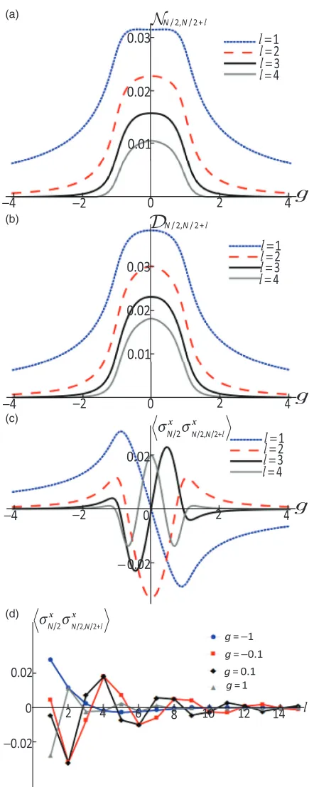
We first consider how Fig. 6 is modified when <1. Figure 7 shows the behavior of entanglement, discord, and correlation functions for=0.05, close to the isotropic limit. As discussed above, theσ_N/x ₂σ_N/x _2+lstill show the odd-even symmetry, but the vanishing of all correlations at g=0 no longer occurs—the precession axis now lies within the xy plane, and so thexcomponent of spin need not decay to zero. When <1, as in the ground state, entanglement extends over a larger range, i.e., not only between nearest neighbors. In addition, the peak entanglement now occurs near g=0, rather than at |g|>1, i.e., quantum correlations attain their maximal value away from the equilibrium quantum critical point [74]. In addition, the peak value of entanglement (and all correlations) is significantly smaller than that seen at=1. From Fig. 7(c) it is clear that at large negative g there is again short-range ferromagnetic order, and antiferromagnetic order at large positiveg. At smallerg, just as seen at=1, the short-range ordering is incommensurate [see Fig. 7(d)]. However, the value of|g|required to see FM/AFM order is larger for =0.05 than it was for =1, so thatg= ±1 now shows incommensurate order. The correlations do still respect the sublattice duality discussed earlier. In contrast to the behavior at =1, the correlations always have a small magnitude [compare the scale of Figs.7(c)and7(d)as compared to Fig.3]. This is consistent with the observation that for =0.05,˜κ=0.5, the mean-field theory would predict the trivial state independent of the value ofg(see Fig.4).

N

−

−

g

l

l

=

l

=

l

=

l

=

D

−

−

g

l

l=

l

=

l

=

l

=

−

−

g

−

σ

_σ

l _l= l=

l=

l=

σx _σx l

l

−

− −

(a)

(b)

(c)

(d)

FIG. 7. (Color online) Evolution of quantum correlations with transverse fieldgnear the isotropic limit=0.05. Panels (a) and (b) show negativityNand geometric quantum discordDas in Fig.6. Panel (c) shows spin-spin correlation σx

jσ x

j+las in Fig. 3. Panel

(d) shows spatial dependence of correlations for the anisotropicXY

model. Parameters (in units of J): ˜κ=0.5 and MPO calculation performed for theN=40 site chain, withχmax=20.

must remain finite as long as is nonzero [36]. The same behavior is indeed seen in the nonequilibrium steady state: For any nonzero, entanglement only extends over a finite range;

l

=

D

Δ

l

=

l

=

l

=

l

=

l

=

Δ

N

(a)

(b)

FIG. 8. (Color online) Evolution of quantum correlations with anisotropy . Panel (a) shows negativity N and (b) geometric quantum discord D. Parameters (in units of J): g= −1,κ˜ =0.5 and MPO calculation performed for the N=40 site chain, with

χmax=20.

this range grows asshrinks and diverges at→0. This can be seen in Fig.8which shows the evolution of entanglement and discord as a function offor various different separations between sites.

As anticipated above, the limit →0 is special, since corresponds to pumping strength. Specifically, as→0, the range over which entanglement exists continues to grow, but the magnitude of the entanglement for any pair of sites ultimately vanishes. Thus the limit→0 is singular, with diverging range of correlations, but vanishing magnitude. The vanishing of negativity, and in fact of all correlations, at=0 can be easily understood from the equation of motion: At= 0, the Hamiltonian conserves numbers of excited two-level systems, while the dissipation reduces this number, so the steady state must be the trivial empty state, which is a product state and thus uncorrelated.

The origin of growing range of negativity can be found by examining the structure and scaling of the two-site density matrix. We first note that this density matrix has a simple structure:

ρij =

⎛ ⎜ ⎜ ⎜ ⎝

p₁₁ 0 0 x₄

0 p₁₀ x₅ 0 0 x∗₅ p01 0

x₄∗ 0 0 p00.

⎞ ⎟ ⎟ ⎟

This structure is due to a symmetry of the equation of motion, under the transformation ρ→Rρˆ Rˆ with ˆR =_jσ_jz. The consequences of such a symmetry for the Hamiltonian were previously discussed [5]; the decay terms we consider also respect this symmetry. Consequently the steady-state density matrix should satisfy [R,ρ]=0. Tracing over all but two sites, [σ_izσ_jz,ρij]=0, which imposes the structure discussed above. A state of the form (11) is entangled if and only if either p₁₀p₀₁ <|x₄|2_orp

00p11 <|x5|2. In the limit of smallthe excited state populationsp11,p01,p10∼2 and so p00∼1. The off-diagonal matrix elements scale as |x4| ∼,|x5| ∼ 2_{. All of these expressions have prefactors that depend on the} separation between sites. However, regardless of these prefac-tors, the scaling ofp₀₁,p₁₀,x₄withimplies that as→0, the first of the two criteria above will always be satisfied, i.e., for any pair of sites, there exists acsuch that for 0< < c they will be entangled. Furthermore, as discussed in Sec.IV, this behavior can be derived analytically within a spin-wave approximation.

E. Correlations vs decay rate

Having explored the dependence on the parameters,g, we conclude our discussion of numerical results by presenting the dependence of quantum correlations on the decay rate ˜κ = κ/J. Figure9shows the evolution with decay rate atg= −1, and the two values ofshown in detail above. Whereas the discord decreases monotonically with decay rate, the behavior

˜

κ

N

Δ Δ

D

˜

κ

Δ Δ

(a)

(b)

FIG. 9. (Color online) Evolution of quantum correlations with ˜κ. Panel (a) shows negativityN, and panel (b) shows geometric quantum discordD, for both Ising limit and small anisotropy limit. Parameters (in units of J): g= −1 and MPO calculation performed for the

N=40 site chain, withχmax=20.

of the negativity depends on anisotropy. In particular, in the Ising limit, there is a nonmonotonic dependence, exhibiting a separable but nonclassical state for sufficiently small ˜κ. The appearance of nonzero entanglement with increasing ˜κ corresponds to the conditionp01p10 = |x4|2: on increasing ˜κ, the probabilities p01 ≡p10 decrease while |x4| varies little at small ˜κ. Nonmonotonic dependence of entanglement on decay rate has also been seen in other contexts [57]. Note that the decay terms remain important even at ˜κ →0. In this limit the steady state is only attained at long times; the state which is finally attained is still determined by the open system dynamics.

IV. ASYMPTOTIC→0 BEHAVIOR AND SPIN-WAVE APPROXIMATION A. Spin-wave calculation of negativity

As noted above, for =0, the NESS of our model corresponds to an empty state. This suggests that for small an approximation based on a low density of excited two-level systems can be used: a bosonic spin-wave approach [54]. This corresponds to reverting from two-level systems (hard core bosons) to bosonic fieldsσ_j−→bˆj. Equation (2) thus becomes

H_eff = − j

[g(2 ˆb†_jbˆj−1)+( ˆbj†bˆj+1+bˆ†j+1bˆj)

+( ˆb†_jbˆ†_j+1+bˆj+1bˆj)]. (12)

This approximation is valid as long as double occupancy of a site can be ignored. Fourier transforming both this and the loss term, the master equation can be written as

dρ dt = −i

k hk,ρ

+κ˜ k

[2 ˆbkρbˆ†k−bˆk†bˆkρ−ρbˆ†kbˆk],

(13)

hk = −

ˆ b†_k bˆ₋k

g+cos(k) cos(k) cos(k) g+cos(k)

ˆ bk ˆ b₋†_k

,

so that each pair of modesk,−kform a closed subsystem. To find steady-state correlations, we replace the density matrix equation of motion, Eq. (13), by equivalent Heisenberg-Langevin equations [55]. The Heisenberg-Heisenberg-Langevin equations can be derived by writing the Heisenberg equations for the system operators coupled to a Markovian bath. After eliminating the dynamics of the bath operators, one finds equations for the system operators of the form

d

dtbˆk=i[hk+h−k,bˆk]−κ˜bˆk+

√

2 ˜κbˆin_k(t). (14)

The Markovian bath has two effects: It causes decay of the system operator ˆbk at the rate ˜κ, and it introduces an “input noise” term ˆbin

k(t). Since we consider decay into a zero-temperature (i.e., empty) bath, there is only vacuum quantum noise: The only nonzero noise correlation function is bˆin

k(t) ˆb† in

and ˆb₋†_kcan be written in a matrix form, ˙ˆ

f(t)=Mfˆ(t)+mˆ(t), (15) in which ˆf(t) is the column vector comprising operators ˆbk(t) and ˆb†_−k(t), ˆm(t) is the column vector containing the noise operators:

ˆ

f(t)=( ˆbk(t), bˆ†_−k(t))T,

ˆ

m(t)=√2 ˜κbˆin k(t),

√

2 ˜κbˆ†₋in_k(t)T; and the matrixMis given by

M=

−κ˜+2i[g+cos(k)] 2icos(k)

−2icos(k) −κ˜−2i[g+cos(k)]

.

The solution of Eq. (15) is fˆ(t)=eMt_fˆ(0)+

t 0eM

(t₋t)_{mˆ(t)dt. Since the real parts of the eigenvalues}

of M are negative, the first of these terms vanishes in the long-time limitt → ∞. In this limit one then finds

ˆ bk(t)

√

2 ˜κ = t

0

dtG1(t−t) ˆb_kin(t)+G2(t−t) ˆb₋†in_k(t), (16) ˆ

b₋†_k(t)

√

2 ˜κ = t

0

dtG₁∗(t−t) ˆb†₋in_k(t)+G₂∗(t−t) ˆb_kin(t),

where the propagatorsG1,2(τ) are matrix elements of exp(Mτ). By introducing the dispersions k=2[g+cos(k)],ηk= 2cos(k), ξk= 2k−η2k,the propagators can be written as

G1(τ)=e−κτ˜

cos(τ ξk)+ik

sin (τ ξk) ξk

,

G2(τ)=iηke−κτ˜ sin(τ ξk)/ξk.

To find the quantum correlations of the state, we first note that since the problem involves noninteracting bosons, the steady state is Gaussian, i.e., it can be fully characterized by the covariance matrix Vj,k as given below. Introducing ˆxj =

ˆ

b_j +bˆ†_j,ˆp_j =( ˆb_j −bˆ†_j)/ iwe have

Vj,k =

Aj Cj k CTj k Ak

, Cj k =

xjxks xjpks

xkpjs pjpks

, (17)

and Aj =Cjj, where xps = xp+px/2. To find these correlators, it is sufficient to find bˆ†_jbˆj+l and bˆjbˆj+l. In the real space the correlatorbˆ_j†bˆj+lcan be expressed as

bˆ†_jbˆ_j+l = 1 N

k,k

bˆ†_kbˆ_kei(k _−k)j

eikl. (18)

Using Eq. (16) one finds that forN → ∞,

_bˆ† jbˆj+l =

1 4π

π

−π η2

k ξ_k2+κ˜2dk e

ikl_,

(19)

and a similar expression forbˆ_jbˆj+l. By substitutingeik→z, the integral becomes a contour integral around the unit circle

|z| =1, so its value depends on the residue of those polesz= Z with|Z|<1. The four poles come in complex conjugate pairs and can be found in closed form Z=ζ ±ζ2−_1, where ζ =[g±g22−_κ˜2₍₁−2_)/4]/(1−2_{). Two of}

these poles which we denote as Z0,Z∗0 lie within the unit circle, and in terms of these one finds

bˆ†_jbˆj₊l =2[α(Z0)l−1+α∗(Z∗0)l−1], (20)

bˆjbˆj+l =β(Z∗₀)l−1, (21)

whereα,βare complex functions of ˜κ,,g. We have factored out the asymptotic scaling withat→0. Since|Z0|<1, all correlations decay exponentially with separationn.

The definition of negativity given earlier, Eq. (5), is specific to qubits, i.e., two-level systems. For a Gaussian state an alternate definition of negativity can be found in terms of the symplectic eigenvalue ˜ν2

−=(τ−

τ2−_{4 Det[Vj,j}

+l])/2,

whereτ =Det[Aj]+Det[Aj+l]−2 Det[Cj,j+l]. The state is separable if ˜ν₋>1, and so negativity for such states may be defined asN =max(0,1−ν˜₋). Using the asymptotic scaling of the elements of the covariance matrix with, we find that in the→0 limit

˜

ν₋ 1−4|bˆjbˆj₊l|, N 2|bˆjbˆj₊l|. (22)

Within this limit, it is thus clear thatN >0 for all pairs of sites, butN ∝and soN vanishes at small, reproducing the singular behavior found numerically in the previous section.

κ=

σ− _σ−

+ −

Δ

κ=

κ=

κ=

κ=

κ=

˜

κ

ξc (a)

(b)

FIG. 10. (Color online) (a) Correlation lengthξc at=0.005

B. Comparing spin-wave approximation to numerics The spin-wave theory relies on neglecting effects of possible double occupation of a given site. While the prob-ability of such an event is small for →0, it is not a prioriclear whether its effects are negligible, since the pair creation term creates excitations on adjacent sites, hence hopping can easily create a doubly occupied site within the bosonic approximation. For this reason, we compare the results of the MPO numerics and the spin-wave theory in the limit→0.

We focus on the correlation function σ_j−σ_j−_+l, or its equivalent bosonic form, which according to Eq. (22) de-termines the asymptotic negativity as →0. Both MPO and spin-wave results show this correlation function decays exponentially with separation l (neglecting edge effects). Consequently this correlation function can be character-ized by its value for nearest neighbors l=1 (N.B. the l=0 case vanishes by definition), and by its correlation length ξc, defined as |σ_j−σ_j−_+l| ∝e−l/ξc_{. In the spin-wave}

theory ξc= −1/ln|Z0|. These two characteristic quantities are shown in Fig. 10, focusing on the limiting behavior at→0.

The correlation length shown in Fig. 10 shows that the spin-wave theory accurately reproduces the results of the numerics, and both show a diverging correlation length (|Z0| →1) in the limit ˜κ→0. In contrast, the magnitude of correlations (i.e., prefactors of the exponential decay) do not match well except at ˜κ 1. This can be explained as follows: At small ˜κ, excitations created on adjacent sites can easily hop to create doubly occupied sites, thus rendering the bosonic approximation inaccurate. For ˜κ1, excitations on adjacent sites are lost before hopping can create doubly excited sites.

V. CONCLUSIONS

In the present work we have studied the nonequilibrium steady state of a parametrically driven 1D coupled cavity array. Making use of an MPO representation to determine the open system evolution, we obtain the nonequilibrium steady state of a dissipative transverse field Ising model. The steady state can be related to the ground state configuration for transverse field g <0, and to the maximum energy configuration for g >0. Consequently, for either sign of g, many features of the quantum correlations behave similarly to those in the ground state Ising model. The most significant difference is that dissipation destroys the phase transition, and so no critical behavior occurs at|g| =1 with correlation lengths remaining finite. We have also compared the results of the MPO numerics with the predictions of the mean-field theory. Mean-field theory erroneously predicts long-range ordered phases, but the nature of the ordering predicted is reflected by the MPO numerics. We have identified a singular limit, of weak driving, where the range of quantum correlations diverges, but the magnitude of the correlations vanishes. This limiting behavior can be recovered analytically from a spin-wave theory, which accurately recovers the correlation length in this limit.

ACKNOWLEDGMENTS

C.J. and J.K. acknowledge support from EPSRC programme “TOPNES” (EP/I031014/1), and EPSRC (EP/G004714/2). F.N. acknowledges support from the EPSRC grant “A Pragmatic Approach to Adiabatic Quantum Computa-tion” (EP/K02163X/1). J.K. acknowledges helpful suggestions from R. Fazio and hospitality from MPI-PKS, Dresden. We acknowledge discussions with A. G. Green, C. A. Hooley, and S. H. Simon.

[1] S. Sachdev,Quantum Phase Transitions, 2nd ed. (Cambridge University Press, Cambridge, 2011).

[2] L. P. Kadanoff, Statistical Physics: Statistics, Dynam-ics and Renormalization (World Scientific, Singapore, 2000).

[3] M. A. Nielsen and I. L. Chuang,Quantum Computation and Quantum Information(Cambridge University Press, Cambridge, 2010).

[4] A. Osterloh, L. Amico, G. Falci, and R. Fazio,Nature (London)

416,608(2002).

[5] T. J. Osborne and M. A. Nielsen,Phys. Rev. A. 66, 032110 (2002).

[6] G. Vidal, J. I. Latorre, E. Rico, and A. Kitaev,Phys. Rev. Lett.

90,227902(2003).

[7] L. Amico, A. Osterloh, and V. Vedral,Rev. Mod. Phys.80,517 (2008).

[8] R. Horodecki, P. Horodecki, M. Horodecki, and K. Horodecki, Rev. Mod. Phys.81,865(2009).

[9] H.-P. Breuer and F. Petruccione,The Theory of Open Quantum Systems(Oxford University Press, Oxford, 2002).

[10] W. H. Zurek,Rev. Mod. Phys.75,715(2003).

[11] R. Lo Franco, B. Bellomo, S. Maniscalco, and G. Compagno, Int. J. Mod. Phys. B27,1345053(2013).

[12] F. Dimer, B. Estienne, A. S. Parkins, and H. J. Carmichael,Phys. Rev. A75,013804(2007).

[13] M. J. Hartmann,Phys. Rev. Lett.104,113601(2010).

[14] K. Baumann, C. Guerlin, F. Brennecke, and T. Esslinger,Nature (London)464,1301(2010).

[15] D. Nagy, G. K´onya, G. Szirmai, and P. Domokos,Phys. Rev. Lett.104,130401(2010).

[16] S. Diehl, A. Tomadin, A. Micheli, R. Fazio, and P. Zoller,Phys. Rev. Lett.105,015702(2010).

[17] S. Ferretti, L. C. Andreani, H. E. T¨ureci, and D. Gerace,Phys. Rev. A82,013841(2010).

[18] T. E. Lee, H. H¨affner, and M. C. Cross,Phys. Rev. A84,031402 (2011).

[19] D. Marcos, A. Tomadin, S. Diehl, and P. Rabl,New J. Phys.14, 055005(2012).

[20] K. W. Murch, U. Vool, D. Zhou, S. J. Weber, S. M. Girvin, and I. Siddiqi,Phys. Rev. Lett.109,183602(2012).

[22] T. Grujic, S. R. Clark, D. Jaksch, and D. G. Angelakis,New J. Phys.14,103025(2012).

[23] E. G. Dalla Torre, E. Demler, T. Giamarchi, and E. Altman, Phys. Rev. B85,184302(2012).

[24] E. G. Dalla Torre, S. Diehl, M. D. Lukin, S. Sachdev, and P. Strack,Phys. Rev. A87,023831(2013).

[25] A. Le Boit´e, G. Orso, and C. Ciuti,Phys. Rev. Lett.110,233601 (2013).

[26] J. Jin, D. Rossini, R. Fazio, M. Leib, and M. J. Hartmann,Phys. Rev. Lett110,163605(2013).

[27] T. E. Lee, S. Gopalakrishnan, and M. D. Lukin,Phys. Rev. Lett.

110,257204(2013).

[28] S. Genway, W. Li, C. Ates, B. P. Lanyon, and I. Lesanovsky, arXiv:1308.1424[Phys. Rev. Lett. (to be published)].

[29] A. Hu, T. E. Lee, and C. W. Clark,Phys. Rev. A88,053627 (2013).

[30] M. J. Hartmann, F. G. S. L. Brand˜ao, and M. B. Plenio,Nat. Phys.2,849(2006).

[31] A. D. Greentree, C. Tahan, J. H. Cole, and L. C. L. Hollenberg, Nat. Phys.2,856(2006).

[32] D. G. Angelakis, M. F. Santos, and S. Bose,Phys. Rev. A76, 031805(2007).

[33] M. J. Hartmann, F. G. S. L. Brand˜ao, and M. B. Plenio,Laser Photonics Rev.2,527(2008).

[34] S. Schmidt and J. Koch,Ann. Phys.525,395(2013).

[35] C.-E. Bardyn and A. Imamo˘glu,Phys. Rev. Lett.109,253606 (2012).

[36] J. Maziero, H. C. Guzman, L. C. C´eleri, M. S. Sarandy, and R. M. Serra,Phys. Rev. A82,012106(2010).

[37] P. Stelmachovic and V. Buzek,Phys. Rev. A70,032313(2004). [38] K. Le Hur,Ann. Phys323,2208(2008).

[39] G. Vidal,Phys. Rev. Lett.91,147902(2003). [40] G. Vidal,Phys. Rev. Lett.93,040502(2004). [41] S. R. White,Phys. Rev. Lett.69,2863(1992). [42] S. R. White,Phys. Rev. B48,10345(1993).

[43] M. A. Cazalilla and J. B. Marston,Phys. Rev. Lett.88,256403 (2002).

[44] S. R. White and A. E. Feiguin, Phys. Rev. Lett.93, 076401 (2004).

[45] A. J. Daley, C. Kollath, U. Schollw¨ock, and G. Vidal,J. Stat. Mech.(2004)P04005.

[46] A. Micheli, A. J. Daley, D. Jaksch, and P. Zoller,Phys. Rev. Lett.93,140408(2004).

[47] S. R. Clark and D. Jaksch, Phys. Rev. A 70, 043612 (2004).

[48] Z. Cai and T. Barthel,Phys. Rev. Lett.111,150403(2013).

[49] U. Schollw¨ock,Ann. Phys.326,96(2011).

[50] M. Zwolak and G. Vidal,Phys. Rev. Lett.93,207205(2004). [51] R. Or´us and G. Vidal,Phys. Rev. B78,155117(2008). [52] T. Prosen and M. ˇZnidariˇc,J. Stat. Mech.(2009)P02035. [53] M. P. A. Fisher, P. B. Weichman, G. Grinstein, and D. S. Fisher,

Phys. Rev. B40,546(1989).

[54] D. C. Mattis,The Theory of Magnetism Made Simple(World Scientific, Singapore, 2006).

[55] M. O. Scully and M. S. Zubairy,Quantum Optics(Cambridge University Press, Cambridge, 1997).

[56] J. Cresser,J. Mod. Opt.39,2187(1992).

[57] C. Joshi, M. Jonson, P. ¨Ohberg, and E. Andersson,Phys. Rev. A

87,062304(2013).

[58] A. Peres,Phys. Rev. Lett.77,1413(1996).

[59] M. Horodecki, P. Horodecki, and R. Horodecki,Phys. Lett. A

223,1(1996).

[60] C. Lupo, V. Man’ko, G. Marmo, and E. Sudarshan,J. Phys. A: Math. Gen.38,10377(2005).

[61] R. Josza and N. Linden,Proc. R. Soc. London, Ser. A459,2011 (2003).

[62] H. Ollivier and W. H. Zurek, Phys. Rev. Lett. 88, 017901 (2001).

[63] L. Henderson and V. Vedral,J. Phys. A.: Math. Gen.34,6899 (2001).

[64] K. Modi, A. Brodutch, H. Cable, T. Paterek, and V. Vedral,Rev. Mod. Phys.84,1655(2012).

[65] E. Knill and R. Laflamme,Phys. Rev. Lett.81,5672(1998). [66] B. Daki´c, Y. O. Lipp, X. Ma, M. Ringbauer, S. Kropatschek,

S. Barz, T. Paterek, V. Vedral, A. Zeilinger, C. Brukner, and P. Walther,Nat. Phys.8,666(2012).

[67] B. Daki´c, V. Vedral, and C. Brukner, Phys. Rev. Lett. 105, 190502(2010).

[68] F. B. F. Nissen, Ph.D. thesis, University of Cambridge, 2013. [69] M. J. Hartmann, J. Prior, S. R. Clark, and M. B. Plenio,Phys.

Rev. Lett.102,057202(2009).

[70] M. J. Bhaseen, J. Mayoh, B. D. Simons, and J. Keeling,Phys. Rev. A85,013817(2012).

[71] N.B., the measure that we use, negativity, and that used in Refs. [4,5], concurrence, are not identical. We have checked that plotting concurrence instead of negativity does not affect any of the conclusions discussed here.

[72] J. Ma, X. Wang, C. P. Sun, and F. Nori,Phys. Rep.509,89 (2011).

[73] T. Yu and J. H. Eberly,Science323,598(2009).