A bistable reaction diffusion system in a stretching flow

Stephen M. Cox

and Georg A. Gottwald

1_{School of Mathematical Sciences, University of Adelaide, Adelaide 5005, Australia}

2_{School of Mathematics and Statistics, University of Sydney, NSW 2006, Australia}

March 14, 2006

Abstract

We examine the evolution of a bistable reaction in a one-dimensional stretching flow, as a model for chaotic advection. We derive two reduced systems of ordinary differential equations (ODE’s) for the dynamics of the governing advection–reaction–diffusion partial differential equation (PDE), for pulse-like and for plateau-like solutions, based on a non-perturbative approach. This reduction allows us to study the dynamics in two cases: first, close to a saddle–node bifurcation at which a pair of nontrivial steady states are born as the dimensionless reaction rate (Damk¨ohler number) is increased, and, second, for large Damk¨ohler number, far away from the bifurcation. The main aim is to investigate the initial-value problem and to determine when an initial condition subject to chaotic stirring will decay to zero and when it will give rise to a nonzero final state. Comparisons with full PDE simulations show that the reduced pulse model accurately predicts the threshold amplitude for a pulse initial condition to give rise to a nontrivial final steady state, and that the reduced plateau model gives an accurate picture of the dynamics of the system at large Damk¨ohler number.

PACS: 82.20.-w; 82.40.Bj

Keywords: reaction–diffusion system, chaotic stirring, bistable chemical reaction

Correspondence to: Dr S M Cox, School of Mathematical Sciences, University of Adelaide, Ade-laide 5005, Australia; tel +61 8 8303 6417; fax +61 8 8303 3696;[email protected]

1

Introduction

In natural and industrial environments active processes such as chemical or biological reactions are often embedded in a fluid flow. Examples include mixing of reactants within continuously fed or batch reactors [1, 2], the development of plankton blooms and occurrence of plankton patchiness [3–6], increased depletion of ozone caused by chlorine filaments [7] and flame fila-mental structures in combustion systems [8]. The fluid flow is very often time-dependent and stirring. This gives rise to interesting effects, and the presence of compression and stirring in chaotic flows typically leads to filamentation of the chemical or biological components. This evidently changes the reaction dynamics. The filamentation caused by the chaotic advection leads to an increased surface area of the reacting components and an increase of the reaction output. However, if the stirring rate is too strong, the filaments become thinner and thinner and the reaction may stop. The corresponding flow-mediated saddle–node bifurcation has been reported in [9–16].

A natural question in such stirred reactions is: Given a chaotic flow environment and an initial distribution of chemical or biological reactants, is it possible to predict whether the reaction will take place and develop or whether it will die out? This question is of paramount importance in an environmental context where the reactants may be ozone in the atmosphere or pollutants in the ocean, or in an industrial context where one is interested in maximizing the reaction output. This problem is well-studied in the non-stirred case [17]. However, so far the complex nature of chaotic flows has prohibited an analytical treatment of this problem in the stirred case.

In principle, these phenomena can be studied directly in a two- or three-dimensional reaction– advection–diffusion system, albeit with huge computational effort. An analytical treatment of the full system is prohibited by the complicated nature of the underlying equations, which involve multiple-scale processes. Simplified models are needed to capture essential features of the influence of the stirring on the reaction kinetics. In filamental or lamellar models [18], the two-dimensional problem of reacting tracers is replaced by a one-dimensional problem of the form

∂

∂tui−λx ∂

∂xui =Di ∂2

stir-ring rate λ. Such models have been applied by several groups, to autocatalytic, bistable and excitable media in several physical, chemical and biological contexts [4,5,9–14]. Phenomenolog-ical filamental models such as (1) can be justified by the following consideration: The chaotic advection causes filaments to be stretched in one direction and compressed in another. In the stretched direction, the concentration is homogenized and gradients along the filaments can be neglected. This motivates a one-dimensional reduction for the concentration in the direction transverse to the filament, subject to the effect of stirring and compression. The parameter

λ can be thought of as the Lagrangian mean strain in the contracting direction, and may be argued to be given by the absolute value of the negative Lyapunov exponent or the (slightly larger) topological entropy. For a different approach to this problem see [19, 20]. The validity of such simplified models has been numerically investigated in [21].

In this paper we study a bistable model withn = 1 and_F1(u1;k1) =k1u1(u1−1)(α−u1) in (1). The solutions of this model are found to be generically either of a plateau-like or a pulse-like character. Plateau solutions are found stably when the stirring rate is low compared to the reaction rate. Pulse-like solutions are found close to the saddle–node bifurcation, where the stirring rate is strong enough to suppress the reaction; moreover the unstable solution for weak stirring rates is also of a pulse-like character. The unstable solution will be of interest when we consider the initial-value problem and ask when an initial perturbation will develop into a plateau-like solution. We extend a non-perturbative approach developed in [26] to derive from (1) a corresponding low-dimensional system of ordinary differential equations which describes the time evolution of plateau-like and pulse-like solutions. We determine the equilibrium solutions, accurately describe the saddle–node behaviour and derive an analytical expression for the asymptotic width of a stationary front. By studying the phase-portrait of the reduced system we are able to determine the fate of various initial concentration profiles in (1); these predictions are then verified numerically by comparison with simulations of the full partial differential equation (1).

2

The model

In this paper we study a bistable model

∂ ∂tu−x

∂

∂xu=D ∂2

∂x2u+ Dau(u−1)(α−u), u(x, t)→0 asx→ ±∞, (2)

where 0< α < 1. The Damk¨ohler number Da =k/λ measures the ratio of the time scales of fluid motion and reaction: small Damk¨ohler numbers correspond to fast stirring/slow reaction, while for large Damk¨ohler numbers the system behaves asymptotically like an unstirred system.

The ODE corresponding to (2) in the absence of spatial effects has two stable fixed points,

u= 0 and u= 1, which are separated by an unstable fixed point at u =α. For the unstirred case of the PDE (2), the system is well known and well described in textbooks such as [22–25]: an initial perturbation which is larger than α over a finite range will spread over the whole domain if 0 < α < 0.5; by contrast, if 0.5 < α < 1, an initial perturbation will decay to the stable state u = 0. The stirred case is much less well understood, and the initial-value problem has to our knowledge never been analytically treated. The stirred case was investigated numerically in [5, 10], and semi-analytically in [15]: stationary fronts between the

u= 0 and u= 1 states exist as a balance between the x-dependent stirring and the diffusion-mediated counterpropagating fronts, for large enough values of the Damk¨ohler number. An initial sufficiently large perturbation seeded at x = 0 spreads as a pair of fronts, driven by its reaction kinetics and diffusion, until the fronts reach the locations x = _±ν where their velocities equal the ambient spatially dependent velocity of the chaotic stirring.

It has been observed in [10,15] that there is a critical Damk¨ohler number such that no stationary pulses exist for Da < Dac, i.e., when the time scale of the chaotic advection, τf = 1/λ, becomes too short in comparison with the time scale of the reaction, tr = 1/k. For large Damk¨ohler numbers, an asymptotic expression for the scaling of the total concentration was developed in [10]. However, the techniques used in [10] cannot describe the behaviour close to the bifurcation point Da = Dac. Moreover, these techniques are stationary and cannot answer questions about the evolution of initial perturbations of reactants.

0 0.2 0.4 0.6 0.8 1

-6 -4 -2 0 2 4 6

u(x)

x

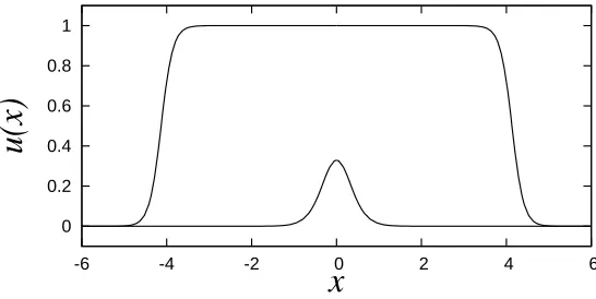
Figure 1: The two nontrivial steady states of (2) for α = 0.2 and Da = 100. The ‘pulse’ solution is unstable; the ‘plateau’ solution is stable.

2.1

Asymptotic steady states for large

Da

We aim to find steady states u(x) that satisfy

xux+Duxx+ Dau(α−u)(u−1) = 0, u(x)→0 asx → ±∞, (3)

when Da1. Numerical simulations show that for Da1 the stable solution is plateau-like and the unstable solution is bell-shaped (see Figure 1).

For the unstable bell-shaped solution u=V(x), we introduce

X =√Dax

so that (3) becomes

DVXX +V(α−V)(V −1) = 0,

with an error of order Da−1. We may now readily determine the appropriate leading-order solution, which gives rise to

V(x) = 3α

  

1 +α+q1

2(1−2α)(2−α) cosh

 

s

αDa

D x

 

  

−₁

+_O(Da−₁

). (4)

We note that this gives

V(0)_∼3α

1 +α+q1₂(1₋2α)(2₋α)

−1

which we shall later compare with a corresponding result obtained from a reduced test function ansatz using a bell-shaped test function, derived in Section 4.

In the large-Da limit, the plateau solutionu=U(x) is, to leading order in Da, given byU = 1 in a region ₋ν < x < ν and U = 0 outside this region, where ν =√Daω, for some ω=_O(1). The locations of the interfaces are determined by a balance between the tendency of the pulse to spread (with constant velocity) and the compressive effects of the imposed velocity field (for which the velocity is proportional to x) [10, 15]; we return to this point in more detail in Section 5.1.1. Around x = _±ν there are transition regions of width _O(1/√Da). To analyse the region aroundx=ν, we introduce

ξ=√Da(x₋√Daω).

Then from (3) we obtain

DUξξ+ωUξ+U(α−U)(U −1) = 0,

with an error of order 1/√Da. Correspondingly,

U(ξ) = 1₂1₋tanhhξ/√8Di, (6)

with ω = qD/2(1 ₋2α). There is a similar transition region near x = ₋ν. We shall in Section 5 use tanh profiles such as these as an ansatz for our second reduced model; since the ansatz captures exactly the large-Da form of the fronts, we shall find correspondingly that the reduced model provides an excellent approximation to the dynamics of the full PDE (2).

Figure 1 shows the solutions of (2) obtained by a shooting algorithm for high Damk¨ohler number (Da = 100). It clearly shows that the stable solution is plateau-like and the unstable solution is pulse-like. Note that the stable solution for smaller Da, close to the bifurcation (not shown here), is also pulse-like.

2.2

Asymptotic solutions for small

Da

0 0.2 0.4 0.6 0.8 1

-4 -3 -2 -1 0 1 2 3 4

u(x)

x

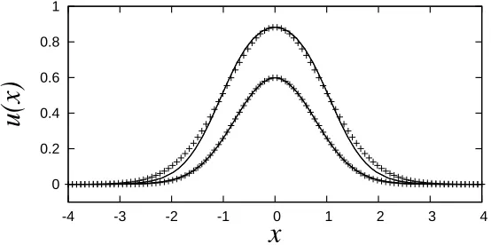
Figure 2: The two nontrivial steady states of (2) forα= 0.2 and Da = 10; the upper and lower solutions are, respectively, stable and unstable. Shown in each case with crosses are fits to a Gaussian.

bifurcation point, i.e., for Da<Dac, no steady-state solutions exist, and any initial condition decays to zero. In fact, if we expand the solution as a series in the Damk¨ohler number according tou(x, t) = Dau0(x, t) +O(Da2), the equation is satisfied at leading order by

u0(x, t) =f0(t) exp(−(w0(t)x)2), (7)

where w0 → 1/

√

2D and f0 → 0 as t → ∞; the latter limit reflects the nonexistence of nontrivial steady states for Da < Dac. Although Dac = _O(10), which is clearly not small, it seems that the leading-order term (7) provides an accurate representation of the solution to (2) close to the saddle–node point Da = Dac – see Figure 2. So in the first instance we shall approximate both stable and unstable solutions close to the saddle–node point by a Gaussian; we shall later consider, in somewhat less detail, other possible profiles of ‘bell-shaped’ form.

Using a non-perturbative method developed in [26] we now derive a set of ordinary differential equations which describe the dynamics of these plateau- and pulse-like solutions. In the next section we briefly explain this variational approach.

3

Nonperturbative, variational method

to the bifurcation point the pulse shape is approximately a bell-shaped function. Numerical simulations and the asymptotic analysis in Section 2.1 and 2.2 show that this is also the case for the bistable model (2) close to the saddle–node bifurcation at which the stable and unstable solutions are born, and on the unstable branch at large Damk¨ohler numbers. A test-function approximation that optimises the two free parameters of a bell-shaped test-function, i.e., its amplitude and its width, allows us to find the actual bifurcation point, Dac, and determine the pulse shape for close-to-critical pulses at Damk¨ohler numbers near Dac. We note that the framework of asymptotic techniques, such as inner and outer expansions where the solution is separated into a steep narrow front and a flat plateau, are bound to fail close to the bifurcation point, because the pulse is clearly bell-shaped, and such a separation is no longer possible. We shall make explicit use of the shape of the pulse close to the critical point and parameterise the pulse appropriately.

We choose u(x, t) of the general form

u(x) =f(t)U(η) with η=w(t)x , (8)

where U(η) is a symmetric, bell-shaped function of unit width and height, and f(t) is the amplitude of the pulse. Close to the saddle–node bifurcation and for the unstable solution at large Damk¨ohler numbers, the solution is indeed a bell-shaped pulse, which we approximate by a Gaussian (see Figure 2). However, our results do not depend on the specific choice of the test function, and the numerical values differ only marginally when sech-functions are used instead, for instance (see Figure 5). We restrict the solutions to a subspace of a bell-shaped function f U(η), which is parameterised by the amplitude, f(t), and the inverse pulse width,

w(t). The evolution of these parameters is then determined by minimizing the error made by the restriction to the subspace defined by (8); this is achieved by projecting (2) onto the tangent space of the restricted subspace, which is spanned by ∂u/∂f =U and ∂u/∂w =f ηUη/w. We set to zero the integral of the product of (2) with the basis functions of the tangent space (over the entire η-domain). This leads to ordinary differential equations for f(t) and w(t); it also yields an approximation to the critical Damk¨ohler number Dac.

function a combination of tanh-functions

u(x, t) = 1

2f(t) [tanh(η+a(t))−tanh(η−a(t))] with η=w(t)x, (9) where a(t) = w(t)ν(t) and the fronts are located around x = _±ν. In a manner analogous to that described above for a pulse ansatz, the variational approach allows us in this case to determine the time evolution of the solution amplitude f(t), the inverse interface width w(t) and the front locations_±ν(t) by projecting (2) onto the tangent space of the restricted solution subspace, which is now spanned by∂u/∂f, ∂u/∂w and ∂u/∂ν.

4

Stable and unstable pulse solutions

Near the turning point at Da = Dac(α), both nontrivial steady-state solutions take the form of bell-shaped pulses near x = 0. We note that in the literature a pulse commonly refers to a stable homoclinic solution; however, here we use the term merely to mean a bell-shaped function, regardless of whether it is stable or unstable. This terminology allows us to distinguish between the two test function ans¨atze (8) and (9).

To determine a reduced model for such pulse solutions, we therefore introduce the ansatz (8) and to determine the evolution of f(t) and w(t) we enforce the vanishing of the two inner products

h(ut−xux−Duxx−Dau(α−u)(u−1))ufi = 0

h(ut−xux−Duxx−Dau(α−u)(u−1))uwi = 0,

where

uf ≡

∂u

∂f =U, uw ≡

∂u

∂w =

f wηU

0

, _{h· · ·i ≡}

Z ∞

−∞· · · dη.

For a Gaussian pulse, with U(η) = e−_η2

, we note the requisite integrals

hUm_i=

π

m

1/2

, _hU02

i=

π

2

1/2

, _hη2U02

i= 3 4

π

2

1/2

.

Thus after some algebra we find thatf(t) and w(t) evolve according to

˙

f = f

−Daα₋2Dw2+ 7₃Da(1 +α)q1₆f ₋5₄Daq1₂f2

(10)

˙

w = w

1₋2Dw2₊1

3Da(1 +α)

q

2 3f−

1 2Da

q

1 2f

In order to examine the dynamics of this system in the phase plane it is useful for brevity of notation to write it in the form

˙

f = fn₋µ1−µ2w2+µ3f −µ4f2

o

(12)

˙

w = wnλ1 −λ2w2+λ3f −λ4f2

o

, (13)

and note that the µi and λi are all positive; also µ2 = λ2 (this equality does not necessarily hold for other profiles U(η)).

We now examine the steady states (w, f) = (w, f) of (12), (13) and their stability. Note that the steady-state problem has been considered previously [15], although only the solutions identified below as ‘P4’ were considered there. Although not all steady states of (12), (13) correspond to distinct physical solutions, they help us to map out the structure of the phase plane, and hence determine the dynamics of (12), (13).

P1: (w, f) = (0,0)

This steady state exists for all parameter values, and a linearisation aboutP1 yields the eigen-values λ1 and −µ1. Therefore P1 is a saddle point, unstable to perturbations in w and stable to perturbations in f.

P2: (w, f) = ((λ1/λ2)1/2,0)

This steady state exists for all parameter values. A linearisation about this point yields the eigenvalues₋µ1−µ2λ1/λ2 <0 and −2λ1 <0. Thus P2 is a stable node.

P3: w= 0, f 6= 0

Here

µ4f 2

−µ3f +µ1 = 0. (14)

This quadratic has two real, positive solutions

f− =

f+ =

µ3+ (µ23−4µ4µ1)1/2 2µ4

,

for all parameter values; indeed f− and f₊ are independent of Da. Note that, since P3 corre-sponds to infinitely wide pulses (w= 0), the roots of the quadratic would be α and 1 if there were no approximation due to the Gaussian pulse ansatz. A linearisation about either steady state yields the eigenvalues

e1 ≡(µ3−2µ4f)f , e2 ≡(λ1+λ3f−λ4f 2

).

Nowµ3−2µ4f± =∓(µ2₃−4µ4µ1)1/2, so the eigenvaluee1indicates stability forf+and instability for f− (e₁ corresponds to perturbations in f, with w ≡ 0). The eigenvalue e₂ corresponds to disturbances in w and satisfies

µ4e2 = (λ3µ4−λ4µ3)f + (λ4µ1+λ1µ4);

it seems to indicate instability for f+ and either stability or instability for f−, depending on the parameter values.

P4: w6= 0, f 6= 0

Heref satisfies

(µ4−λ4)f 2

−(µ3−λ3)f+µ1+λ1 = 0. (15)

We note the coefficients (cf. [15])

µ4−λ4 = 3Da

4√2, µ3−λ3 =

5Da(1 +α)

3√6 , µ1+λ1 = 1 + Daα. (16)

The quadratic (15) has two real, positive roots provided

α < αm ≡

1₋2q₋√1₋4q

2q ≈0.47448, whereq =

25 81√2,

and

Da>Dapulse_{c ≡}hq(1 +α)2₋αi−1.

In this case, we denote the two solutions of (15) byf∗ + > f

∗

−. Correspondingly w=w∗

±, where

µ2w ∗ ±

2

=₋µ4f ∗ ± 2

+µ3f ∗

±−µ1. (17)

Since the right-hand side of (17) must be non-negative, we deduce, by comparison with (14), that each off∗

− and f ∗

+ lies between f− and f₊. At Da = Dapulse_c , the two solutions collide in a saddle–node bifurcation; no such solutions exist for Da<Dapulse_c .

A linearisation about either of theP4 steady states yields, forf =f+δf(t) andw=w+δw(t), that

δf˙ = (µ3f −2µ4f 2

)δf ₋2µ2wf δw

δw˙ = (λ3−2λ4f)w δf −2λ2w2δw.

Hence the growth rateσ satisfies

σ2+bσ+c= 0, (18)

where

b= 2λ2w2−µ3f+ 2µ4f 2

=₋2µ1+µ3f

and

c= 2µ2w2f(2(µ4−λ4)f −(µ3−λ3)).

Note that for f∗

+, c > 0; for f ∗

−, c < 0, indicating instability. The bifurcation point c = 0 corresponds to (the limitsw= 0 or f = 0 or) Da = Dapulse_c . Note that σ=_O(Da) as Da_{→ ∞}.

Two phase planes for (12), (13) illustrating the saddle–node bifurcation at Dac are shown in Figure 3. If Da < Dapulse_c , the fixed points P4 do not exist, and all initial conditions off the f-axis asymptote to the solution (w,0) at large time (physically the trivial state u _≡ 0). If instead Da > Dapulse_c , the P4 solutions exist, and there is a separatrix that divides initial conditions leading to the physically trivial state (w,0) from those leading to the physically nontrivial state (w∗

+, f ∗ +).

w

f

*

w

separatrix

f

f

+

−

f

(w ,f )

(w ,f )

Figure 3: Two of the possible phase planes for (12), (13) illustrating the saddle–node bifurca-tion. Left: Da<Dapulse_c , and the fixed points P4 do not exist. Right: Da>Dapulsec .

0.3 0.4 0.5 0.6 0.7 0.8 0.9 1 1.1 1.2

10 15 20 25 30 35 40

max

u(x)

Da

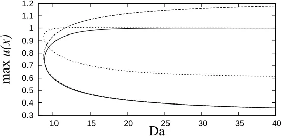
Figure 4: Comparison between the steady states of (2) computed by shooting (solid line), the pulse model (15) (dashed line) and the plateau model (30) (dotted line). Hereα= 0.2.

we show that good agreement is also given for different ans¨atze such as U(η) = sechnη. We thus conclude that the actual form of the pulse shape is not particularly important (and hence we cannot expect to deduce this pulse shape from any asymptotic theory).

0.3 0.4 0.5 0.6 0.7 0.8 0.9 1 1.1 1.2

8 10 12 14 16 18 20 22 24

max

u(x)

Da

Figure 5: Comparison between different shaped pulses in the model (15). The solid curve represents the steady states of (2) computed by shooting; the dashed lines represent solutions of the pulse model (15) for test functions U(η) = e−_η2

, sech2η and sech4η (respectively from right to left at the saddle–node bifurcation point). Parameters as in Figure 4.

0 0.2 0.4 0.6 0.8 1

0 0.1 0.2 0.3 0.4 0.5

max

u(x)

α

5

Plateau solutions

Away from the saddle–node bifurcation, the stable solution takes the form of a nearly uniform region aroundx= 0, surrounded by a pair of fronts. This solution may be captured by writing

u(x, t) in the form

u(x, t) = 1₂f(t)φ(η) with η=w(t)x, (19)

where

φ(η) = tanh(η+a(t))₋tanh(η₋a(t)).

Then the evolution of f(t), w(t) and ν(t) = a/w (or, equivalently, f, w and a) may be determined by forcing the inner products of (2) with each of uf,uw and uν to be zero, where

uf =

∂u ∂f =

1

2φ(η) =

u f

uw =

∂u

∂w =

1 2f

h

(x+ν) sech2(η+a)₋(x₋ν) sech2(η₋a)i

uν =

∂u ∂ν =

1

2f wψ(η),

with

ψ(η) = sech2(η+a) + sech2(η₋a).

The corresponding steady-state calculation has been considered in [15]; here we extend their analysis to the time-dependent problem. This permits us to determine which initial conditions lead to excitation and which to extinction. Details of our derivation, including analytical expressions for all the requisite inner products, are given in the Appendix: we find that the equations for the time evolution of f, w and ν take the form

λ1wf˙+λ2fw˙ +λ3w2fν˙ = wf

h

λ4+λ5Dw2+ Da(λ6+λ7f+λ8f2)

i

(20)

µ1wf˙+µ2fw˙ +µ3w2fν˙ = wf

h

µ4+µ5Dw2+ Da(µ6+µ7f +µ8f2)

i

(21)

β1wf˙+β2fw˙ +β3w2fν˙ = wf

h

β4+β5Dw2+ Da(β6+β7f +β8f2)

i

. (22)

5.1

Steady states

We shall not attempt here a full analysis of the three-dimensional phase space for f, w andν; instead we consider only nontrivial steady-state solutions for whichf,wand ν are all nonzero. We expect two such solutions when Da exceeds some threshold, one stable and one unstable. We shall consider the dynamics of (20)–(22) later.

The equations for the (nontrivial) steady states may be written in the form

λ4+λ5Dw2+ Da(λ6+λ7f+λ8f2) = 0 (23)

µ4+µ5Dw2+ Da(µ6+µ7f+µ8f2) = 0 (24)

β4+β5Dw2+ Da(β6 +β7f +β8f2) = 0. (25)

These equations are readily solved without recourse to nonlinear root finding, for example in the following way. First we fix values for α and a. Then we use (23) to write

w2 ₌ −λ4−Da(λ6+λ7f +λ8f2)

λ5D

. (26)

Then, upon substitution of this expression forw2 _{in (24), we have}

µ0

4+ Da(µ 0 6+µ

0 7f+µ

0

8f2) = 0, where µ 0

i =µi−

µ5

λ5

λi. (27)

Likewise

β0

4+ Da(β 0 6+β

0 7f+β

0

8f2) = 0, where β 0

i =βi−

β5

λ5

λi. (28)

Now by eliminating Da between (27) and (28), we find the following equation for f:

(µ04β 0 8−µ

0 8β

0

4)f2+ (µ 0 4β

0 7−µ

0 7β

0

4)f+µ 0 4β

0 6 −µ

0 6β

0

4 = 0, (29)

which is of the form

A(a)f2+ (1 +α)B(a)f+αC(a) = 0. (30)

The quadratic equation (30) needs careful interpretation. First we note that the coefficients

0.6 0.7 0.8 0.9 1

0 20 40 60 80 100 120 140

f

Da

0 5 10 15 20 25

0 20 40 60 80 100 120 140

a

Da

1 1.5 2 2.5 3 3.5 4 4.5

0 20 40 60 80 100 120 140

w

Da

0 1 2 3 4 5

0 20 40 60 80 100 120 140

ν

Da

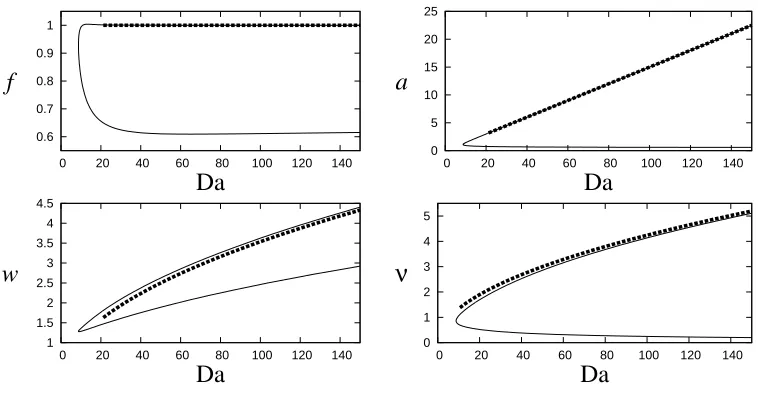
Figure 7: Steady-state solutions of the plateau model (23)–(25) (solid line) for α = 0.2. The dashed lines give large-Da asymptotics (32), (33) of the plateau model for the upper branch. The asymptotic results are indistinguishable from the numerical results for f and a.

(26) the corresponding values ofw, we find numerically that the root of (29) corresponding to positive Da seems always to give rise to w2 _{>0, and so is indeed physically reasonable. Thus} we emphasise that both branches of solutions evident in Figures 7 and 8 arise fromone of the roots of (30) for fixed α, as a is increased monotonically.

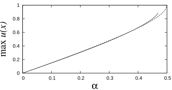
The steady states for α= 0.2 (see [15]) are shown in Figure 7. Note that solutions exist only for Da> Daplateau_c (α). Figure 8 shows steady-state solution branches for a range of values of

α. The excellent agreement between solutions of the plateau model and steady states of (2) on the upper branch is illustrated in Figures 4 and 9. Of course, we expect a tanh-test function ansatz to fail close to the bifurcation point Dac where the solution rather is bell-shaped and is accurately described by a Gaussian ansatz as in Section 4.

Of particular interest is the limit of large Damk¨ohler number, Da 1. The numerics suggest the following scalings. On the upper branch of solutions

a= ¯aDa, w= ¯wDa1/2, f = ¯f , (31)

where ¯a,w,¯ f¯=_O(1); on the lower branch

a= ˜a, w= ˜wDa1/2, f = ˜f,

0.2 0.3 0.4 0.5 0.6 0.7 0.8 0.9 1 1.1

0 10 20 30 40 50 60

f

Da

1

2

3

4

Figure 8: Steady-state solutions of the plateau model (23)–(25) for α= 0.1,0.2,0.3,0.4. (The corresponding value of 10α is indicated next to each curve.)

5.1.1 Large Damk¨ohler number, Da1, upper branch

We now construct the plateau solutions on the upper branch, in the limit Da 1. In that limit, we find

λ4 ∼ −a µ4 ∼ ₁₈1π2− 1₃ β4 ∼ −2₃a

λ5 ∼ −2₃ µ5 ∼ −1₃ β5 →0

λ6 ∼ −2aα µ6 ∼ −1₂α β6 ∼ −α

λ7 ∼2(1 +α)a µ7 ∼ ₂1(1 +α) β7 ∼ 2₃(1 +α)

λ8 ∼ −2a µ8 ∼ −11₂₄ β8 ∼ −1₂.

Recall thata=_O(Da). The result forβ5 indicates that this quantity is exponentially small in Da. Thus at leading order in Da we have, from (23)–(25),

−α+ (1 +α) ¯f ₋f¯2 = 0

−1 3Dw¯

2₊1

2(−α+ (1 +α) ¯f − 11 12f¯

2_{) = 0}

−23¯a+ (−α+ 2

3(1 +α) ¯f − 1 2f¯

2_{) = 0.}

The first of these equations gives ¯f = 1 or ¯f =α; the latter solution must be rejected since the last equation would then give ¯a =₋(2₋α)α/4< 0. The choice ¯f = 1 is consistent with our numerical calculations, which indicate that this is the solution relevant to the upper branch. With ¯f = 1, the remaining equations give Dw¯2 ₌ 1

8 and ¯a = 1

4(1−2α). Thus in the large-Da limit,

f _∼1, w_∼

Da

8D

1/2

0 0.2 0.4 0.6 0.8 1

-3 -2 -1 0 1 2 3

u(x)

x

Figure 9: Comparison between stable steady states of the plateau model (crosses) and of the advection–reaction–diffusion equation (2) (solid line). Here α = 0.4 and Da = 100.0359 (implied by our choice of a); for the plateau-model solution, a = 5.0, f = 1.000179 and

w= 3.62460.

Note, as a consequence, that for large Da we have

ν _∼√2DDa1_{2 −}α, (33)

in agreement with the phenomenological argument given in [10, 15]. This formula can be understood if we note that the location of a stationary front is given approximately through a balance between the front velocity v0 =

√

2DDa1 2 −α

of the unstirred problem [10] and the velocity of the chaotic stirring (i.e., x in the scaling of (2)). Thus in the stirred problem, the front has zero velocity when v0 =x, which impliesv0 =ν, and (33) follows.

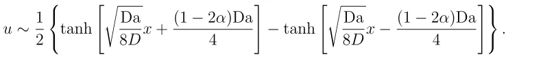
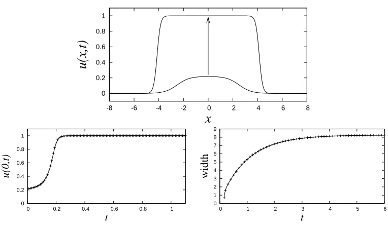
Finally, the solution takes the form

u_∼ 1

2

  

tanh

 

s

Da 8Dx+

(1₋2α)Da 4



−tanh  

s

Da 8Dx−

(1₋2α)Da 4

 

  

. (34)

A comparison between this expression and a numerical calculation of the stable steady state of (2) is shown in Figure 9; to graphical resolution, the two graphs are indistinguishable.

0 0.002 0.004 0.006 0.008 0.01

20 40 60 80 100 120 140 160 180 200 220

Da

width

Figure 10: Comparison between the width of the steady-state solution as obtained from the plateau model and from the advection–reaction–diffusion equation (2). Here α = 0.4. Shown is 2(νapprox−νexact) against the Damk¨ohler number Da.

number, which is expected, because the tanh-front ansatz gets closer to the actual solution, which asymptotically is a pair of tanh-fronts (see Section 2.1).

Solutions of the plateau model on the lower branch are of less interest because they do not correspond closely to steady-state solutions of the full PDE, where the unstable solution is pulse-like.

5.2

Stability

Suppose that (f, w, ν) is a nontrivial steady state of (20)–(22) (i.e., f, w, ν ₆= 0). Since the various coefficients in (20)–(22) are functions ofa, it is useful to consider the linearised evolution of δf,δw and δa, where in the linearisation δa=wδν+νδw. Thus we have

λ1wδf˙+λ2f δw˙ +λ3f w(δa˙ −νδw˙) = Daf w(λ7+ 2λ8f)δf + 2Df w2λ5δw

+f wn∂λ4 +Dw2∂λ5+ Da(∂λ6+f ∂λ7+f2∂λ8)

o

δa,

where

∂λi ≡

∂λi

and where all nonperturbation quantities are evaluated at the fixed point. There are two further equations, withλi 7→µi and λi 7→βi. The three may be written together as

A     

δf˙ δw˙

δa˙

     =_B      δf δw δa      ,

where the constant-coefficient matrices_Aand _B are readily determined from the three pertur-bation evolution equations.

5.2.1 Large Damk¨ohler number, Da1, upper branch

On the upper solution branch, in the limit Da1, we have

A ∼     

2aw ₋a w

1 2w

1

18(π2 −6) 0

w ₋2₃a 2₃w

    

, _{B ∼}

    

−2Dawa(1₋α) ₋4 3Dw

2 _−w

1

12Daw(6α−5) − 2

3Dw2 0

−13Daw(1−2α) 0 −

2 3w      ,

where the zero entries indicate terms that are exponentially small in Da. Thus, in view of the scalings (31), A ∼     

2¯aw¯Da3/2 ₋a¯Da w¯Da1/2 1

2w¯Da 1/2 1

18(π

2_{−6) 0}

¯

wDa1/2 ₋2₃a¯Da 2₃w¯Da1/2

     and B ∼     

−2 ¯wa¯(1₋α)Da5/2 ₋4 3Dw¯

2_{Da −w¯Da}1/2 1

12w¯(6α−5)Da 3/2

−23Dw¯2Da 0

−13w¯(1−2α)Da

3/2 ₀

−23w¯Da 1/2

     .

It then follows (after some algebra) that

A−₁

B ∼         

−(1₋α)Da ₋2Dw¯ 3¯a Da

−_1/2 0 3 ¯w

2(π2₋₆₎Da 3/2

−_2(π23

−6)Da 0

3¯a

2(π2₋₆₎Da 2

−12_π2Dw¯a¯ −6Da

3/2

−1          .

We require the dominant eigenmodes of _A−₁

B. There are three eigenvalues:

The eigenvector corresponding to Λ1 has δf =δw= 0 and δa= 1, say; thus disturbances in a decay like e−_t

. We find Λ2 ∼ −(1−α)Da; recalling the scalings f =O(1), w =O(

√

Da) and

ν = _O(√Da), we find that the associated eigenvector has (δf, δw, δa) _∼ (F, WDa1/2, ADa), with

−(1₋α) + 3

2(π2₋₆₎

!

W = 3 ¯w

2(π2₋₆₎F and −(1−α)A = 3¯a

2(π2₋₆₎F −

12Dw¯¯a π2₋₆W.

The final eigenvalue is

Λ3 ∼ − 3

2(π2₋₆₎Da,

with eigenvector (δf, δw, δa)_∼(F, WDa3/2, ADa2), where

−_2(π23

−6)+ 1−α

!

F =₋2Dw¯

3¯a W and A= 8Dw¯¯aW.

Note that this calculation confirms the stability of the upper branch solution, since Λ1,2,3 <0. Furthermore, the scalings (35) confirm the observation from numerical simulations of the PDE (2) that the relaxation of the front separation to its equilibrium value is slower than the relaxation of either the amplitude of the solution or the width of each front. (Provided the fronts are reasonably well separated initially, numerical integrations of either the PDE or the system (20)–(22) indicate that first f adjusts to approximately its long-time value; then w

adjusts to give each front the appropriate width, and finally a adjusts so that the fronts are separated by the correct distance.)

Since 0< α < 1₂ and since 3₂(π2₋₆₎−₁

≈0.3876, we have

|Λ2|>|Λ3| |Λ1|.

6

Comparison between dynamics of the reduced models

and the full PDE

Our models extend the steady-state analysis of [15] by providing approximations to the

dy-namics of the PDE (2). This allows us to examine the evolution of initial conditions which

0.2 0.25 0.3 0.35 0.4 0.45 0.5

0 0.2 0.4 0.6 0.8 1 1.2

f

w

Figure 11: Comparison between the separatrix f = fpulse

s (w) determined from the Gaussian pulse ansatz (continuous line) and the threshold f = fPDE

s (w) obtained from simulations of the full PDE (2) (crosses) with initial profileu(x,0) =fe−_(wx)2

as a function ofw; parameter values areα = 0.2 and Da = 16.

initial pulse-like solution we may now solve the initial-value problem at Damk¨ohler numbers close to the critical Damk¨ohler number Dac, where both stable and unstable solutions are well approximated by a bell-shaped function. We can readily compute the corresponding separa-trix in (w, f)-space between those solutions that asymptote at large times to the uniform zero solution, and those that asymptote to a nontrivial steady state. We denote the separatrix by

f = fpulse

s (w). For initial conditions (w(0), f(0)) below the separatrix the solution will die out, whereas for initial conditions above the separatrix the reaction will continue and develop into a stable stationary pulse. It is of particular interest to determine the extent to which this result provides useful corresponding information for the full PDE (2). We have therefore carried out a large number of simulations of the PDE, each from a Gaussian initial condition

u(x,0) = fe−_(wx)2

, in an effort to compute a corresponding separatrix: f = fPDE

s (w). For a given value ofw, we use bisection to determine approximately the corresponding value off that delineates the two large-time behaviours. The results, and a comparison with the separatrix from the Gaussian pulse ansatz, are given in Figure 11. The agreement is excellent. There is similar agreement at higher Da; for example, at Da = 100, and w(0) = 1, the Gaussian ansatz gives a threshold f(0) = 0.2537, while from the PDE we find 0.2525_±0.0005.

0 0.2 0.4 0.6 0.8 1

-8 -6 -4 -2 0 2 4 6 8

u(x,t)

x

0 0.2 0.4 0.6 0.8 1

0 0.2 0.4 0.6 0.8 1

u(0,t)

t

0 1 2 3 4 5 6 7 8 9

0 1 2 3 4 5 6

width

t

Figure 12: Comparison between numerical simulations of the PDE (2) and the plateau model (20)–(22). Top: initial and final states, with arrow indicating direction of temporal evolution. Bottom left: u(0, t) against time. Bottom right: ‘width’ of the pulse, 2ν. In each of the lower plots, PDE results are given by a solid line and plateau-model results by crosses.

by the ODE

du

dt = Dau(α−u)(u−1),

so that f is initially decreasing if f(0) < α and increasing if f(0) > α. Thus the threshold value off(0) leading to zero or nonzero large-time states is rather triviallyf(0)_≈α.

The agreement between the plateau model and the full PDE is remarkable because, as shown in Section 2.1, the unstable solution is pulse-like and not plateau-like. Furthermore, as shown in Figure 4, the unstable solution predicted by the plateau model is quantitatively incorrect. However, some insight into the agreement may be obtained by noting that the unstable pulse-like steady-state has eigenvalues σ =_O(Da), which are large in the limit Da_{→ ∞}, and which indicate that the associated instability is reaction-dominated. Our simulations of the PDE (2) confirm that the initial condition illustrated in Figure 12 first rapidly undergoes an adjustment of the central concentration to u _≈ 1, consistent with a time scale _O(1/Da), then a slower relaxation of the front width and location.

7

Conclusions

We have developed reduced systems of ordinary differential equations describing the time evolution of both plateau-like and pulse-like solutions of a one-dimensional bistable reaction– diffusion partial differential equation for a stirred flow environment. The PDE possesses a trivial steady state in which all the reactant is used up, and, when the dimensionless reaction rate Da is great enough, a pair of nontrivial steady states, one stable and one unstable, born in a saddle–node bifurcation at Da = Dac. The pulse model was shown to provide a good approximation close to the bifurcation point and for the unstable steady solution at large Da. The plateau model applies for large Da, and captures well the form of the stable steady state. By studying equilibrium pulse solutions, we were able to accurately describe the bifurcation behaviour of the system near Dac. For large Damk¨ohler numbers our reduced plateau model allowed us to describe the stationary fronts, and derive a commonly used phenomenological formula for the width of a stationary front.

Appendix

Here we record some details of the derivation of the coefficients in the plateau model (20)– (22). We begin by noting that wuw = 1₂f ηφ

0

(η) +νφν = 1₂f(ηφ 0

+wνψ), xux = 1₂f ηφ 0

(η) and

uxx = 1₂f w2φ 00

(η).

Now we list the various inner products that are needed for the calculation:

hu2_fi = 1_4hφ2_i

huwufi =

f

4wh(ηφ

0

+wνψ)φ_i=₋ f 8whφ

2

i+f ν 4 hψφi

huνufi = 1₄f whψφi

hηφ0ufi = 1₂hηφ 0

φ_i=₋1_4hφ2_i

hφ00

ufi = 1₂hφ 00

φ_i=₋1 2hφ

02

i hu(α₋u)(u₋1)ufi = 1₄f

h

−α_hφ2_i+1

2(1 +α)fhφ 3

i − 1 4f

2

hφ4_ii hu2_wi = f

2 4w2

h

hη2φ02

i+ 2wν_hηφ0

ψ_i+w2ν2_hψ2_ii huνuwi = 1₄f2hηφ

0

ψ_i+ 1 4f

2_wν

hψ2_i

hηφ0

uwi =

f

2whη

2_φ02

i+ f ν 2 hηφ

0

ψ_i

hφ00

uwi =

f

2whφ

00 (ηφ0

+wνψ)_i=₋ f 4whφ

02

i − ₄f a_w∂a∂ hφ02

i

hu(α₋u)(u₋1)uwi =

f2 4w a

∂ ∂a −1

! h

−12αhφ 2

i+1₆(1 +α)f_hφ3_{i −16}1 f2_hφ4_ii hu2_νi = 1₄f2w2_hψ2_i

hηφ0uνi = 1₂f whηφ 0

ψ_i

hφ00

uνi = −1₄f w

∂ ∂ahφ

02

i

hu(α₋u)(u₋1)uνi = 1₄f2w

∂ ∂a

h

−1 2αhφ

2

i+ 1

6(1 +α)fhφ 3

i − 1 16f

2

hφ4_ii.

All of the requisite inner products can be found exactly:

hφ2_i = 4(2acoth 2a₋1)

hψφ_i = 1

2

∂ ∂ahφ

2

i= 4 coth 2a₋8acosech22a

hφ02

i = 8

3(1 + 3 cosech 2_2a

−6acosech22acoth 2a)

hφ4_i = 8₃(₋11 + 12acoth32a₋15 cosech22a+ 18acoth 2acosech22a)

hηφ0ψ_i = ₋8₃a hψ2_{i =} 8

3(1−3 cosech

2_{2a+ 6acosech}2_{2acoth 2a)}

hη2φ02

i = 21

9π 2 −2 3 + 4 3a 2 − 4 3a(π

2_{+ 4a}2_{) coth 2acosech}2_2a+ 2 3(π

2_{+ 12a}2_{) cosech}2_2a.

The various coefficients in (20)–(22) are then given by

λ1 = 1₄hφ2i, µ1 =λ2 =−1₈hφ2i+ 1₄ahψφi, β1 =λ3 = 1₄hψφi,

λ4 =−1₈hφ2i, λ5 =−1₄hφ 02

i, λ6 =−1₄αhφ2i, λ7 = 1₈(1 +α)hφ3i, λ8 =−₁₆1 hφ4i,

µ2 = 1₄

h

hη2φ02

i+ 2a_hηφ0

ψ_i+a2_hψ2_ii , β2 =µ3 = 1₄

h

hηφ0

ψ_i+a_hψ2_ii , µ4 = 1₄hη2φ

02

i+ 1₄a_hηφ0

ψ_i, µ5 =−1₈ 1 +a

∂ ∂a

!

hφ02

i, µ6 = 1₈α 1−a

∂ ∂a

!

hφ2_i,

µ7 =−₂₄1(1 +α) 1−a

∂ ∂a

!

hφ3_i, µ8 = ₆₄1 1−a

∂ ∂a

!

hφ4_i,

β3 = 1₄hψ2i, β4 = 1₄hηφ 0

ψ_i, β5 =−1₈

∂ ∂ahφ

02

i,

β6 =−1₈α

∂ ∂ahφ

2

i, β7 = ₂₄1(1 +α)

∂ ∂ahφ

3

i, β8 =−₆₄1

∂ ∂ahφ

4

i.

Acknowledgements G.A.G gratefully acknowledges support by the Australian Research

References

[1] I. R. Epstein, The consequences of imperfect mixing in autocatalytic chemical and biolog-ical systems, Nature 374 (1995) 321–327.

[2] M. A. Allen, J. Brindley, J. Merkin and M. J. Piling, Autocatalysis in a shear flow, Phys. Rev. E 54 (1996) 2140–2142.

[3] E. R. Abraham, The generation of plankton patchiness by turbulent stirring, Nature 391 (1998) 577–580.

[4] A. P. Martin, On filament width in oceanic plankton distributions, J. Plank. Res. 22 (2000) 597–692.

[5] P. McLeod, A. P. Martin and K. J. Richards, Minimum length scale for growth-limited oceanic plankton distributions, Ecological Modelling 158 (2002) 111–120.

[6] E. Hern´andez-Garcia and C. Lop´ez, Sustained plankton blooms under open chaotic flows, Ecological Complexity 1 (2004) 193.

[7] S. Edouard, B. Legras, F. Lef`evre and R. Eymard, The effect of small-scale inhomogeneities on ozone depletion in the Arctic, Nature 384 (1996) 444–447.

[8] P. D. Ronney, Some open issues in premixed turbulent combustion, in Modeling in

Com-bustion Science, pp. 3–22, Eds. J. Buckmaster and T. Takeno (Springer-Verlag Lecture

Notes in Physics, 1994)

[9] Z. Neufeld, Excitable media in a chaotic flow, Phys. Rev. Lett. 87 (2001) 108301–108304.

[10] Z. Neufeld, P. H. Haynes and T. T´el, Chaotic mixing induced transitions in reaction– diffusion systems, Chaos 12 (2002) 426–438.

[11] Z. Neufeld, C. Lop´ez, E. Hern´andez-Garcia and O. Piro, Excitable media in open and closed chaotic flows, Phys. Rev. E 66 (2002) 066208–066220.

[12] E. Hern´andez-Garcia, C. Lop´ez and Z. Neufeld, Filament bifurcations in a one-dimensional model of reacting excitable fluid flow, Physica A 327 (2003) 59–64.

[14] I. Z. Kiss, J. H. Merkin, S. K. Scott, P. L. Simon, S.Kalliadasis and Z. Neufeld, The structure of flame filaments in chaotic flows, Physica D 176 (2003) 67–81.

[15] S. Menon and G. A. Gottwald, Bifurcations in reaction–diffusion systems in chaotic flows, Phys. Rev. E71 (2005) 066201–066207.

[16] W. E. Ranz, Applications of a stretched model to mixing, diffusion, and reaction in laminar and turbulent flows, AIChE J.25 (1979) 41–47.

[17] P. Gray and S. K. Scott,Chemical Oscillations and Instabilities, Clarendon Press, Oxford (1994).

[18] W. E. Ranz, Applications of a stretch model to mixing, diffusion, and reaction in laminar and turbulent flows, AIChE J. 25 (1979) 41–47.

[19] X. Z. Tang and A. H. Boozer, Design criteria of a chemical reactor based on a chaotic flow, Chaos 9 183–194 (1999).

[20] J.–L. Thiffeault, Advection–diffusion in Lagrangian coordinates, Phys. Lett. A 309 415– 422 (2003).

[21] S. M. Cox, Chaotic mixing of a competitive–consecutive reaction, Physica D 199 (2004) 369–386.

[22] J. D. Murray, Mathematical Biology, 2nd edition, Springer Verlag, New York (1993).

[23] J. Keener and J. Sneyd, Mathematical Physiology, Springer Verlag, New York (1998).

[24] A. S. Mikhailov, Foundations of synergetics I: Distributed active systems, 2nd edition, Springer Verlag, Berlin (1994).

[25] A. Scott, Nonlinear Science – Emergence and Dynamics of Coherent Structures, Oxford University Press, Oxford (1999).

[26] G. A. Gottwald and L. Kramer, On propagation failure in one- and two-dimensional excitable media, Chaos 14 (2004) 855–863.