Foreword and Colophon
This paper reports on work performed in 2005–6 by my grad. student Benji Kelly, which eventu-ally formed a major part of his Masters (M.Phil) thesis here at the University of Nottingham. He then went on to do a PhD at Cornell University.
Benji’s work began with an interest in Golomb coding but he soon extended the scope of his researches to take in adaptive binary arithmetic coding. The paper presented here was submitted to the annual Data Compression Conference in 2006 (DCC 2006). These conferences are held in Snowbird, Utah and are very well regarded in the DCC field. Although our paper was accepted only as a poster, we felt rather pleased to have had success of some sort at our first attempt. The version here is the original, unabbreviated, submission to DCC.
The paper was created using LATEX with the hyperref package and was then converted to PDF using pdfeTeX-1.21a
The B-coder: An improved binary arithmetic coder and
probability estimator
Benjamin Kelly and David Brailsford
School of Computer Science and Information Technology
University of Nottingham, Nottingham, UK
{bgk,dfb}@cs.nott.ac.uk
Abstract
In this paper we present the B-coder, an efficient binary arithmetic coder that per-forms extremely well on a wide range of data. The B-coder should be classed as an ‘approximate’ arithmetic coder, because of its use of an approximation to multiplica-tion. We show that the approximation used in the B-coder has an efficiency cost of 0.003 compared to Shannon entropy. At the heart of the B-coder is an efficient state machine that adapts rapidly to the data to be coded. The adaptation is achieved by al-lowing a fixed table of transitions and probabilities to change within a given tolerance. The combination of the two techniques gives a coder that out-performs the current state-of-the-art binary arithmetic coders.
1
Background
Arithmetic coding (AC) is a technique for data compression that theoretically allows us to code data at Shannon entropy. The idea was first developed by Pasco[1], who was inspired by a proof of Shannon’s theorem, and shortly after by Rissanen [2]. The first practical implementation was by Langdon and Rissanen [3]. The basic idea in AC is to represent a series of choices between events as a selection of intervals (or regions) on the real line. Each choice can be viewed as a selection of a letter from an alphabet, α, and arithmetic coding as a way of representing strings fromα∗. For each letter inα, an initial interval is allocated whose length is proportional to its probability. When the first letter is known, its region is selected and re-divided according to suitable probabilities. Langdon and Rissanen were the first to show that the issues of determining probabilities and performing the coding can be dealt with separately [4]. Their suggestion is to use a modelling unit to partition the data into conditioning classes or contexts, such that the members of a particular context share similar characteristics and therefore similar probabilities. An arithmetic coder can then exploit the similarity by coding the members of each class together. In this paper we make contributions to both practical arithmetic coding and probability estimation.
alphabet, where letteri ∈ 0...n−1, has probability P(i), coding the event j proceeds as follows. LetW(j)be the alphabetic index of the jth character of the string to be encoded, thenCandAbecome: Aj = Aj−1×P(W(j))andCj =Cj−1+S(W(j)), whereS(0)=0
andS(k)=Pk−1
l=0 P(l).
Binary arithmetic coding (BAC) is a special case of AC that allows for decisions be-tween two events to be encoded. Conventionally we designate the two events MPS and LPS, for more-probable and less-probable symbol, and letα = {0,1}. The initial region is the semi-open interval [0,1), which is first divided into two regionsL(for the less-probable letter, assumed to be 1 in the equations below) andM(for the more-probable letter, assumed to be 0 in the equations below), such that L +M = 1 covers the entire region. For each event to be coded, the region corresponding to the event to be encoded is selected, and that new region is again divided in to L0 and M0. Note that the division of the region at each coding decision need not be the same, that is, it is not necessary for L+LM = L0+L0M0. This
allows a modelling unit to provide a BAC with a different estimate for LPS for each symbol, which coupled with the interval subdivision allows a BAC to achieve optimal compression without alphabet extension. In terms of the coding variables described above, binary arith-metic coding has a particularly simple implementation. Redefining A be a function from strings ofαi.e. (0,1)∗ to interval size andC to be a function from strings ofα to interval start points,C and Acan be defined using the following double recursion:
A(s0)= A(s)− A(s1) (1)
A(s1)= A(s)×P(1) (2)
C(s0)=C(s) (3)
C(s1)=C(s)+A(s0) (4)
In [3], Langdon and Rissanen developed a binary arithmetic coder, which we refer to as the Skew Coder1. Their motivation was to find a simple implementation of binary arith-metic coding that did not involve multiplication. (In the early days of aritharith-metic coding, the time taken to perform multiplication in hardware was very high compared to other machine operations.) In the skew coder, fixed-point arithmetic is carried out inn-bit registers. When the left-most bit of Ais a zero, both AandC are shifted to the left until the left-most bit of
Ais a one, this overcomes the “growing precision” problem caused by the continual multi-plication in step 2. The simplification in the skew coder is accomplished by approximating the multiplication in equation 2 with a right-logical-shift (). If P(LPS)=2−Q, equation 2 then becomes A(s1) = A(S) Q. The parameter Q is known as the skew value, and is supplied to the arithmetic coder in lieu of the probability estimate for the event to be coded. The skew coder performs surprisingly well on real data, given the crudeness of the approximation.
In search of further speed improvements, the skew coder was refined in [6], where the multiplication is replaced by assignment (and a corresponding shift ofC). In this refinement
1In recent literature there is some confusion about which of Langdon and Rissanen’s coders is the ‘skew
0 1 2 3 4 5 6
0 0.05 0.1 0.15 0.2 0.25 0.3 0.35 0.4 0.45 0.5
Probability of least probable symbol
% over entropy
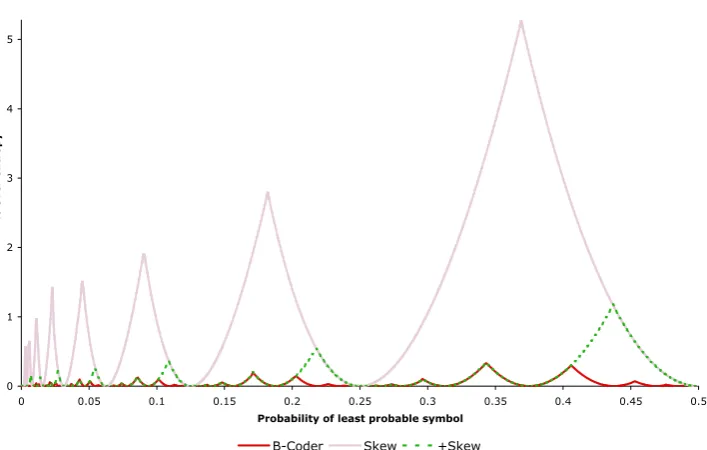
[image:4.595.112.466.99.324.2]B-Coder Skew +Skew
Figure 1: Code length excess of Skew coder and B coder.
can be seen the beginning of the Q-coder [7] and its variants (Q, QM, MQ). In each of these coders multiplication is replaced by assignment, which is possible when Ais kept close to one. This approximation comes with some cost to coding efficiency, but at the time it was considered a worthwhile price to pay to avoid the costly multiplication. The secret weapon of the Q-coder and its descendants lies in their probability estimation; rather than relying on a modeller to supply the probability of each event to be coded, these coders estimate probabilities internally via an efficient state machine.
In this work we describe a new coder, the B-coder, which is based on the skew coder and in its simplest form has a worst case inefficiency of around 0.3% above entropy. The B-coder incorporates an efficient state machine based loosely around the idea of ‘fast-attack’, as used in JPEG [8]. However, unlike previous coders, our state machine allows the proba-bilities and transitions to fluctuate within a given tolerance, which further improves perfor-mance by between 0.1% and 4% depending on the statistics of the data being coded.
In section 2, we give the derivation of the B-coder. Its probability estimation is de-scribed in section 3. Results are presented in section 4 by comparing the B-coder to two other state-of-the-art coders. Finally, section 5 presents the conclusion.
2
Motivation and description of our code
slightly better, but this new approximation still has a noticeable peak near P(l) = 0.437 (see +Skew in figure 1.) Instead, we approximate using P(l) = 2Q ±2−R,R > Q and achieve a much tighter approximation. In terms of coding variables, this new approximation requires a minor modification: equation 2 becomes A(s1) = A(s0) Q± A(s0) R; and the modelling unit now needs to supply two variables,Qand R, to the coding unit. For simplicity, we allow the sign of R to determine whether A(s0) R should be added or subtracted from A(s0) Q. In the description of the algorithm below, we use thesi gnum
function, wheresi gnum(x)=1 if(x >0),−1 if(x <0),0 otherwise.
Encoding Algorithm
The inputs to the encoding are the bit, b, to be encoded, plus Q and R supplied by the modeller.
1. (Initialise) SetC to 0 and Ato all 1s.
2. Computea1 := A Q+si gnum(R)×(A |R|)
3. Computea0 := A−a1
4. Ifb =0 set A :=a1, else ifb=1 set A:=a1 andC :=C +a0.
5. (Renormalise) While the left-most bit of A is zero, setA:= A1 andC :=C 1.
Note, in carrying out the addition of step 4 the quantityC +a0 may overflow then-bit register, so the output shifted from the left end ofC in the renormalisation step should be buffered, and if carry occurs, the carry should be propagated into the buffer. Additionally, as observed in [3] this carry may propagate through the entire buffer, so a method to block the carry must be used (e.g. bit-stuffing.)
Decoding Algorithm
The inputs to the algorithm are the code string plus skew parameters Qand R, supplied by the modeller. The output is the decoded bit,b.
1. (Initialise) Fill registerC with the firstnbits of the code string and fill Awith 1s.
2. Computea1 := A Q+si gnum(R)×(A |R|)
3. Computea0 := A−a1
4. Ifa0>C then setb:=0 and A:=a0. Go to 6.
5. Otherwisea0≤C, setb:=1,C :=C−a1 and A :=a0.
6. (Renormalise) While the left-most bit of A is zero, setA:= A1 andC :=C 1.
3
Probability estimation
In the previous section we described the B-coder without giving any consideration to prob-ability estimation. For efficient compression a coder needs to have an accurate estimate of the probability of each symbol as it is compressed. A computationally ‘cheap’ approach is to use renormalisation-driven probability estimation, first used in the Q-coder (see [9] for a detailed analysis.) The basic idea is that the renormalisation step in the encoding algorithm can be used as a criterion to decide when to perform adaptation. When an LPS event causes a renormalisation (‘LPS-renorm’) we shouldincreasethe LPS probability estimate and for an MPS invoked renormalisation (‘MPS-renorm’) we shoulddecreaseit.
In the Q-coder and its descendants, the probability estimates are used directly when dividing the intervals during the coding process. The B-coder takes a similar approach. In the B-coder, we have constructed a set of Q and R values that that can be used to estimate a range of LPS probabilities. Our table is arranged in a similar fashion to the ‘fast-attack’ (FA) tables of JBIG/JPEG. A table is ‘fast-‘fast-attack’ when an uninterrupted sequence of MPS-renorms rapidly decreases the LPS probability, faster than would be warranted by the equations in [9]. In our tables, an early LPS-renorm moves the coder into a less confident state and two LPS-renorms move the coder into the steady-state mode, where the analysis from [9] is valid.
One characteristic shared by many table-driven probability estimators is that they are inherently static in nature. The estimated probabilities and transitions are drawn from the table and are always used. In the B-coder we break this paradigm and allow the table entries to fluctuate. The coder keeps track of the quantity MPS-renorms−LPS-renorms for each entry in the probability table and uses this figure as a confidence estimate about that probability. If a table entry has a positive confidence estimate, we can be sure that P(LPS) is lower than the table suggests (because we have had a net-positive number of MPS-renorms at this entry before), so we should compensate in some way. One method is to decrease P(LPS) by a small amount. The necessary adjustments can be achieved by letting the skew values change in some controlled manner.
Effective
Probability Occupancy
Confidence Estimate
0.503 (1,-8) 183484 1358 0.492 (1,-7) 183722 -2515 0.484 (1,-6) 178534 -4026 0.375 (2,3) 170421 -16069 0.313 (2,4) 138650 -22321
0.266 (2,6) 93217 -22460
Effective
Probability Occupancy
Confidence Estimate
[image:6.595.106.506.540.659.2]0.109 (3,-6) 103682 9917 0.094 (3,-5) 151080 7556 0.064 (4,10) 155777 5982 0.059 (4,-8) 147105 3360 0.047 (4,-6) 122792 -321 0.030 (5,-10) 92726 -2389
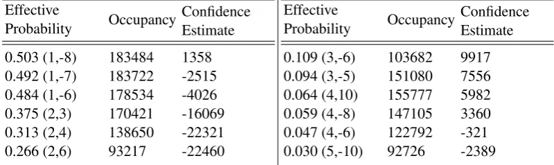
In the B-coder we use the following approach. Compare the confidence estimate with the number of times the context has been used (context occupancy), if the magnitude of the confidence estimate is at least 5% of context occupancy then suitably adjust both Q and R. This technique was motivated by observing the distribution of the probability states that were used during single-context coding (see table 1.) For data distributed with P(LPS) =
0.5, the probabilities used (effective probability) ranged from 2−1 to 2−3. A similar phenomenon was observed during single-context coding of any fixed-probability file, as expected according to the analysis in [9]. In this method, the confidence estimate allows the coder to detect when it using an inappropriate effective probability and compensate proportionally. We found that letting Q and R assume the values from the entry 1 states away in the ‘right’ direction worked best. (The ‘right’ direction is forward if the confidence estimate is positive and backwards if the confidence estimate is negative.) We used the update schedule shown in equation 5 (arrived at experimentally), where confidence level (cl) is confidence estimate/context occupancy.
1 =
0, cl <5 1, 5≤cl <15 2, 15≤cl <35 3, 35≤cl <55 4, 55≤cl
(5)
Even though this schedule and method were derived from single-context coding, we show in the next section that it improves performance even in mixed-context coding.
4
Coding Results and Analysis
To assess the performance of the coder we performed a number of tests on real world data ranging from single context coding through to multi-context bi-level image coding. We present the results in this section. Additionally, for comparison purposes, we include in each test results from the Augmented-ELS coder [10] and the Z-Coder [11]. In the tables of results that follow the entry labelled “B-coder + dynamic state” gives the performance of the coder with the probability model as from section 3. The entry labelled “B-coder + static state” gives the performance of the B-coder with the adaptation disabled, i.e. using only the probabilities and transitions defined by the initial state machine. In each table the best result in each row is underlined.
4.1
Single context coding
P(LPS) Entropy B-coder + static state
B-coder +
dynamic state ELS Coder Z-Coder
0.50 1000000 2.79 1.32 8.38 2.99
0.40 970951 3.04 2.32 8.12 2.52
0.30 881291 2.80 1.77 7.07 2.54
0.20 722656 3.12 1.14 5.13 2.23
0.10 468996 4.85 3.42 3.22 2.17
0.01 80794 4.42 4.28 5.67 3.14
Table 2: A comparison of the B-coder against the ELS- and Z-coder for single context with fixed less probably symbol probabilities. Entropy column is number of bits, coder performance figures are percentage over entropy.
4.2
Bi-level image coding
Bi-level images are a natural source of data for BAC. We developed a simple test suite that modelled images using the JBIG 10-pixel context. Each pixel was assigned a context ac-cording to the values of the pixels “underneath” the template, giving rise to 1024 possible contexts. For the B-coder, each context was allowed its own Q and R values, and main-tained its own set of confidence estimates of the probabilities in the state-machine. Four collections of document images were used:
1. The eight ITU test images (known previously as the “CCITT suite”);
2. 520 pages selected at random from the BBC research and development archive [13] from 1970-1992;
3. 155 pages selected at random from journals available on the JSTOR archive [14];
4. 210 pages selected at random from theses recently completed in the author’s depart-ment.
With the exception of collection 4, the images were all from scanned sources and contained varying levels of noise. The results are presented in table 3.
The B-coder performs best on the first three collections. On the ‘perfect’ images, gen-erated from the theses, the ELS coder does best. For these very clean images, the B-coder isn’t able to adapt to the data as well as the ELS coder; one possible reason for this lies in the results from the previous section. In table 2, we see the ELS coder is able to out-perform the B-coder for LPS probabilities near to 0.10. The context statistics for the clean images involve LPS probabilities near to this value. Overall, the Z-coder is the worst performer.
4.3
Audio residual coding
Test Set B-coder + static state
B-coder +
dynamic state ELS Z-Coder
CCITT 1672944 1670960 1678944 1688856
[image:9.595.176.438.109.201.2]BBC 234551072 233959512 235396960 238096048 JSTOR 34025504 33998744 34146880 34459920 Theses 28562992 28522296 27845664 29558608
Table 3: A comparison of the B-coder against the ELS- and Z-coder coder for bi-level images. File sizes are in bits.
c.0
{0}
c.1
c.2 {1}
{2,3}
c.3
c.4 {4–7}
{8–15}
c.5 c.6
{16–31}
{32–63}
{64–127}
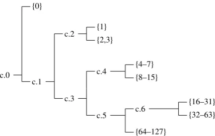
Figure 2: An example decision tree, suitable for coding 7-bit integers.
[15], we developed a coder for monaural audio files. The audio data were split into frames, each 1192 samples long, and 4 finite impulse response predictors were used to predict the contents of each frame. Next, for each frame, the predictor that minimised the difference between the actual frame and the predicted frame was selected and the “residual” values (the difference between a predicted sample and its corresponding actual value) were coded using a BAC. The residuals follow approximately a Laplacian distribution and in the case of 16-bit sampling range from−32768 to +32767 (the range of signed 16-bit integers.) Efficiently coding the residuals using a BAC involved exploiting the distribution of residuals.
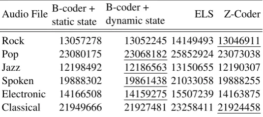
To encode the values, we used a tree structure similar to that shown in figure 2. Notice that the leaves of the tree are sets, S. The BAC was used to encode the decisions (at each c.n) that select the set and alog2(#(S))number was used to encode the position within S, where #(S)denotes the number of elements in S. The signs of the residuals were passed-through the encoder as a 1-bit number. Each of the arithmetic coders was incorporated into this scheme and was used to code audio files from six different genres. The results are presented in table 4.
[image:9.595.198.415.263.400.2]Audio File B-coder + static state
B-coder +
dynamic state ELS Z-Coder
Rock 13057278 13052245 14149493 13046911
Pop 23080175 23068182 25852924 23073038
Jazz 12198492 12186563 13150655 12190307
[image:10.595.173.441.109.228.2]Spoken 19888302 19861438 21033058 19888255 Electronic 14166508 14159275 15507239 14163875 Classical 21949666 21927481 23258411 21924458
Table 4: A comparison of the B-coder against the ELS- and Z-coder for audio residual coding. File sizes are in bytes.
the decision tree structure used to code the residuals results in the context nodes dealing with probabilities in this range.
5
Conclusion and Further work
We have presented the B-coder, an approximate binary arithmetic coder that out-performs other comparable coders on a range of data. Additionally we have demonstrated an im-provement of table-based probability estimation, which allows a probability estimator to better track the source probabilities.
The improvement made in the B-coder’s probability estimation makes a considerable difference in single-context coding (see table 2); where previous coders’ effective prob-ability fluctuated over a large range, the B-coder is able to keep the effective probprob-ability under much tighter control. There are in effect two methods of improving the estimators performance, both using the confidence estimate: (1) allow the probabilities themselves to fluctuate; (2) allow the transitions between the states to fluctuate. In the B-coder, for speed we use technique (1) to achieve technique (2).
The B-coder has reasonable time performance, but our initial implementation was not totally optimised for speed. Our tests show it to be a little faster than the ELS coder, but somewhat slower than the Z-Coder. Possible speed improvements include taking advantage of word size by shifting out blocks of 32-bits at a time. We feel it is necessary to add the following caveat to our work. Recent advances in CPU technology mean that multiplication no longer has the massive cost disadvantage compared with shifts and additions (e.g. for a Pentium-4: IMUL 15µops, ADD+SHIFT 6 µops.) However, in a dedicated hardware device, i.e. when not using a general-purpose CPU, we believe our coder would be an excellent choice. For example, even at the micro-code level, because R is always greater than Q, the shift ofRincludes the shift of Q and this can be exploited.
References
[1] Richard C. Pasco. Source coding algorithms for fast data compression. PhD thesis, Stanford University, Stanford, CA 94305, May 1976.
[2] Jorma Rissanen. Generalized Kraft inequality and arithmetic coding.IBM Journal of Research and Development, 20, 1976.
[3] Glen G. Langdon, Jr. and Jorma Rissanen. Compression of black-white images with arithmetic coding. IEEE Transactions on Communications, COM-29(6):858–867, June 1981.
[4] Jorma Rissanen and Glen G. Langdon, Jr. Universal modeling and coding.IEEE Transactions on Information Theory, 27(1):12–23, Jan 1981.
[5] Ian H. Witten, Radford M. Neal, and John G. Cleary. Arithmetic coding for data compression.
Communications of the ACM, 30(6):520–540, 1987.
[6] Glen G. Langdon, Jr. and Jorma Rissanen. A simple general binary source code. IEEE Trans-actions on Communications, IT-28(5):800–803, September 1982.
[7] W.B. Pennebaker, J.L. Mitchell, G.G. Langdon, Jr., and R.B. Arps. An overview of the basic principles of the Q-Coder adaptive binary arithmetic coder. IBM Journal of Research and Development, 32(6):717–726, November 1988.
[8] William B. Pennebaker and Joan L. Mitchell. JPEG: Still Image Data Compression Standard. Van Nostrang Reinhold, New York, 1993.
[9] W.B. Pennebaker and J.L. Mitchell. Probabilty estimation for the Q-Coder. IBM Journal of Research and Development, 32(6):737–751, November 1988.
[10] W. Douglas Withers. A rapid probability estimator and binary arithmetic coder. IEEE Trans-actions on Information Theory, 47(4):1533–1537, May 2001.
[11] Leon Bottou, Paul G. Howard, and Yoshua Bengio. The Z-coder adaptive binary coder. In
Data Compression Conference, 1998. DCC ’98. Proceedings, pages 13–22, March 1998.
[12] Solomon W. Golomb. Run-length encodings. IEEE Transactions on Information Theory, IT-12(3):399–401, July 1966.
[13] The British Broadcasting Corporation. BBC RD technical reports archive. http://www. bbc.co.uk/rd/pubs/reports/index.shtml.
[14] William G. Bowen. JSTOR and the economics of scholarly communication. http://www. mellon.org/jsesc.html, 1996. See also:http://www.jstor.org.