warwick.ac.uk/lib-publications
Manuscript version: Published Version
The version presented in WRAP is the published version (Version of Record).
Persistent WRAP URL:
http://wrap.warwick.ac.uk/112839
How to cite:
The repository item page linked to above, will contain details on accessing citation guidance
from the publisher.
Copyright and reuse:
The Warwick Research Archive Portal (WRAP) makes this work by researchers of the
University of Warwick available open access under the following conditions.
Copyright © and all moral rights to the version of the paper presented here belong to the
individual author(s) and/or other copyright owners. To the extent reasonable and
practicable the material made available in WRAP has been checked for eligibility before
being made available.
Copies of full items can be used for personal research or study, educational, or not-for-profit
purposes without prior permission or charge. Provided that the authors, title and full
bibliographic details are credited, a hyperlink and/or URL is given for the original metadata
page and the content is not changed in any way.
Publisher’s statement:
Please refer to the repository item page, publisher’s statement section, for further
information.
White Dwarf Rotation as a Function of Mass and a Dichotomy of Mode Line Widths:
Kepler
Observations of 27 Pulsating DA White Dwarfs through
K2
Campaign 8
J. J. Hermes1,6, B. T. Gänsicke2, Steven D. Kawaler3 , S. Greiss2, P.-E. Tremblay2 , N. P. Gentile Fusillo2, R. Raddi2, S. M. Fanale1, Keaton J. Bell4 , E. Dennihy1 , J. T. Fuchs1, B. H. Dunlap1 , J. C. Clemens1, M. H. Montgomery4 ,
D. E. Winget4, P. Chote2, T. R. Marsh2 , and S. Redfield5 1
Department of Physics and Astronomy, University of North Carolina, Chapel Hill, NC 27599, USA;[email protected]
2
Department of Physics, University of Warwick, Coventry CV47AL, UK
3
Department of Physics and Astronomy, Iowa State University, Ames, IA 50011, USA
4
Department of Astronomy, University of Texas at Austin, Austin, TX 78712, USA
5
Wesleyan University Astronomy Department, Van Vleck Observatory, 96 Foss Hill Drive, Middletown, CT 06459, USA
Received 2017 August 7; revised 2017 September 5; accepted 2017 September 5; published 2017 October 9
Abstract
We present photometry and spectroscopy for 27 pulsating hydrogen-atmosphere white dwarfs(DAVs; a.k.a. ZZ Ceti stars)observed by theKeplerspace telescope up toK2Campaign 8, an extensive compilation of observations with unprecedented duration(>75 days)and duty cycle(>90%). The space-based photometry reveals pulsation properties previously inaccessible to ground-based observations. We observe a sharp dichotomy in oscillation mode line widths at roughly 800 s, such that white dwarf pulsations with periods exceeding 800 s have substantially broader mode line widths, more reminiscent of a damped harmonic oscillator than a heat-driven pulsator. ExtendedKeplercoverage also permits extensive mode identification: we identify the spherical degree of 87 out of 201 unique radial orders, providing direct constraints of the rotation period for 20 of these 27 DAVs, more than doubling the number of white dwarfs with rotation periods determined via asteroseismology. We also obtain spectroscopy from 4 m-class telescopes for all DAVs withKeplerphotometry. Using these homogeneously analyzed spectra, we estimate the overall mass of all 27 DAVs, which allows us to measure white dwarf rotation as a function of mass, constraining the endpoints of angular momentum in low- and intermediate-mass stars. Wefind that 0.51–0.73Mewhite dwarfs, which evolved from 1.7–3.0MeZAMS progenitors, have a mean rotation period of 35 hr with a standard deviation of 28 hr, with notable exceptions for higher-mass white dwarfs. Finally, we announce an online repository for our Kepler data and follow-up spectroscopy, which we collect at http:// k2wd.org.
Key words:stars: oscillations –stars: variables: general–white dwarfs
Supporting material:machine-readable tables
1. Introduction
Isolated white dwarf stars have been known for more than half a century to vary in brightness on short timescales
(Landolt 1968). The roughly 2–20 minute flux variations are known to result from surface temperature changes caused by non-radial g-mode pulsations excited by surface convection
(see reviews by Fontaine & Brassard 2008; Winget & Kepler 2008; Althaus et al.2010).
Given the potential of asteroseismology to discern their interior structure, white dwarfs have been the targets of extensive observing campaigns to accurately measure their periods, which can then be compared to theoretical models to probe deep below the surface of these stellar remnants. Early observations of white dwarfs showed pulsations at many periods within the same star, further demonstrating their asteroseismic potential (Warner & Robinson1972). However, observations from single sites were complicated by aliases arising from gaps in data collection.
Starting in the late 1980s, astronomers combated day–night aliasing by establishing the Whole Earth Telescope, a coopera-tive optical observing network distributed in longitude around the Earth acting as a single instrument (Nather et al. 1990). Dozens of astronomers trekked to remote observatories across
the globe for these labor-intensive campaigns, facing complica-tions ranging from active hurricane seasons(O’Brien et al.1998) to near-fatal stabbings(Vauclair et al.2002). Many campaigns lasted up to several weeks with duty cycles better than 70%, delivering some of the most complete pictures of stellar structure and rotation in the 20th century for stars other than our Sun(e.g., Winget et al.1991,1994).
Given the resources required, however, only a few dozen pulsating white dwarfs have been studied with the Whole Earth Telescope. Pulsating hydrogen-atmosphere white dwarfs
(DAVs; a.k.a. ZZ Ceti stars)are the most numerous pulsating stars in the Galaxy, but fewer than 10 were observed with this unified network.
The advent of space-based photometry from CoRoT and Kepler revolutionized the study of stellar interiors, ranging from p-modes in solar-like oscillators on the main sequence and red-giant branch(e.g., Chaplin & Miglio2013)tog-modes in massive stars and hot subdwarfs(e.g., Degroote et al.2010; Reed et al. 2011). For example, from Kepler we now have excellent constraints on core and envelope rotation in a wide range of stars (Aerts2015). We have also seen new types of stochastic-like pulsations in classical heat-driven pulsators, such as δScuti stars (Antoci et al. 2011) and hot subdwarfs
(Østensen et al.2014).
However, this revolution did not immediately translate to white dwarf stars, few of which were identified or observed in
The Astrophysical Journal Supplement Series,232:23(28pp), 2017 October https://doi.org/10.3847/1538-4365/aa8bb5
© 2017. The American Astronomical Society. All rights reserved.
6
the original Kepler mission. We aim to rectify that shortfall with an extensive search for pulsating white dwarfs observable by K2. After the failure of its second reaction wheel, Kepler entered a new phase of observations,K2, where it observes new
fields along the ecliptic every three months (Howell et al. 2014). This has significantly expanded the number of white dwarfs available for extended observations. We targeted all suitable candidate pulsating white dwarfs to provide a legacy of high-cadence, extended light curves.
We present here an omnibus analysis of thefirst 27 DAVs observed by the Kepler space telescope, including follow-up spectroscopy to measure their atmospheric parameters. Only six of the DAVs presented here were known to pulsate prior to theirKeplerobservations, and only two of those six had more than 3 hr of previous time-series photometry.
Our manuscript is organized as follows. In Section 2, we outline our target selection, and we describe our space-based photometry in Section 3. We detail our spectroscopic observations from the 4.1 m SOAR telescope and present our full sample analysis in Section 4. The first part of our light curve analysis, in Section 5, centers on mode stability as a function of pulsation period. We summarize some of the large-scale trends we see in the DAV instability strip as observed by KeplerandK2in Section6. We then explore the asteroseismic rotation periods of 20 of the 27 DAVs in our sample, and place the first constraints on white dwarf rotation as a function of
mass in Section 7. We conclude with notes on individual objects in Section 8, as well as final discussions and conclusions in Section 9. Table 5 in the Appendix features all pulsations discovered and analyzed here: 389 entries corresponding to 201 independent modes of unique radial order(k)and spherical degree(ℓ)in 27 different stars, the most extensive new listing of white dwarf pulsations ever compiled.
2. Candidate DAV Target Selection
Table1 details the selection criteria for the first 27 DAVs observed byKeplerwith short-cadence(∼1 minute)exposures throughK2Campaign 8 and analyzed here, including the Guest Observer(GO)program under which the target was proposed for short-cadence observations.
White dwarfs hotter than 10,000 K are most effectively selected based on their blue colors and relatively high proper motions(e.g., Gentile Fusillo et al.2015). However, only two white dwarfs were known in the 105 square-degreeKeplerfield two years prior to its launch in 2009: WD 1942+499 and WD 1917+461. An extensive search in the year before launch —mostly fromGalexultraviolet excess sources and faint blue objects with high proper motions—uncovered just a dozen additional white dwarfs in the originalKepler field(Østensen et al.2010), with just one pulsating (Østensen et al.2011).
Table 1
Target Selection Criterion for the First 27 Pulsating DA White Dwarfs Observed byKeplerandK2
KIC/EPIC R.A. and Decl.(J2000.0) Alt. g (u–g,g–r) (B–R,R–I) Source K2 Proposal Selection Disc. Name (mag) (AB mag) (AB mag) Catalog Field (GO) Method
4357037 19 17 19.197+39 27 19.10 L 18.2 (0.50,−0.17) L KIS K1 40109 Colors 1 4552982 19 16 43.827+39 38 49.69 L 17.7 L (0.02, 0.03) SSS K1 40050 Colors 2 7594781 19 08 35.880+43 16 42.36 L 18.1 (0.56,−0.16) L KIS K1 40109 Colors 1 10132702 19 13 40.893+47 09 31.28 L 19.0 (0.50,−0.16) L KIS K1 40105 Colors 1 11911480 19 20 24.897+50 17 21.32 L 18.0 (0.43,−0.16) L KIS K1 40105 Colors 3
60017836 23 38 50.740−07 41 19.90 GD 1212 13.3 L L L Eng DDT KnownZZ 4
201355934 11 36 04.013−01 36 58.09 WD 1133−013 17.8 (0.46,−0.17) L SDSS C1 1016 KnownZZ 5 201719578 11 22 21.104+03 58 22.41 WD 1119+042 18.1 (0.39,−0.01) L SDSS C1 1016 KnownZZ 6 201730811 11 36 55.157+04 09 52.80 WD 1134+044 17.1 (0.49,−0.11) L SDSS C1 1015 Spec.Teff 7
201802933 11 51 26.147+05 25 12.90 L 17.6 (0.42,−0.19) L SDSS C1 1016 Colors L 201806008 11 51 54.200+05 28 39.82 PG 1149+058 14.9 (0.45,−0.13) L SDSS C1 1016 KnownZZ 8 206212611 22 20 24.230−09 33 31.09 L 17.3 (0.47,−0.14) L SDSS C3 3082 Colors L 210397465 03 58 24.233+13 24 30.79 L 17.6 (0.65,−0.12) L SDSS C4 4043 Colors L 211596649 08 32 03.984+14 29 42.37 L 18.9 (0.54,−0.18) L SDSS C5 5073 Colors L 211629697 08 40 54.142+14 57 08.98 L 18.3 (0.46,−0.15) L SDSS C5 5043 Spec.Teff L
211914185 08 37 02.160+18 56 13.38 L 18.8 (0.36,−0.21) L SDSS C5 5073 Colors 9 211916160 08 56 48.334+18 58 04.92 L 18.9 (0.40,−0.13) L SDSS C5 5073 Colors L 211926430 09 00 41.080+19 07 14.40 L 17.6 (0.47,−0.20) L SDSS C5 5017 Spec.Teff L
228682478 08 40 27.839+13 20 09.96 L 18.2 (0.35,−0.14) L SDSS C5 5043 Colors L 229227292 13 42 11.621−07 35 40.10 L 16.6 (0.46,−0.12) L ATLAS C6 6083 Colors L 229228364 19 18 10.598−26 21 05.00 L 17.8 L (0.10, 0.03) SSS C7 7083 Colors L 220204626 01 11 23.888+00 09 35.15 WD 0108-001 18.4 L L SDSS C8 8018 Spec.Teff 7
220258806 01 06 37.032+01 45 03.01 L 16.2 (0.41,−0.21) L SDSS C8 8018 Colors L 220347759 00 51 24.245+03 39 03.79 PHL 862 17.6 (0.43,−0.18) L SDSS C8 8018 Colors L 220453225 00 45 33.151+05 44 46.96 L 17.9 (0.42,−0.15) L SDSS C8 8018 Colors L 229228478 01 22 34.683+00 30 25.81 GD 842 16.9 (0.43,−0.19) L SDSS C8 8018 KnownZZ 5 229228480 01 11 00.638+00 18 07.15 WD 0108+000 18.8 (0.45,−0.17) L SDSS C8 8018 KnownZZ 6
References. Discovery of pulsations announced by (1) Greiss et al. (2016); (2) Hermes et al. (2011); (3)Greiss et al. (2014); (4)Gianninas et al. (2006);
(5)Castanheira et al.(2010);(6)Mukadam et al.(2004);(7)Pyrzas et al.(2015)—search for DAVs in WD+dM systems;(8)Voss et al.(2006);(9)Hermes et al.
(2017c).
(This table is available in machine-readable form.)
2
The most substantial deficiency for white dwarf selection came from the lack of existing blue photometry of the Kepler
field, in either SDSS-u¢or Johnson-U; in 2009, there was very little coverage from the Sloan Digital Sky Survey (SDSS) of the Kepler field. Two surveysfilled this gap several years afterKeplerlaunched: theKepler-INT Survey(KIS), providing U–g–r–i–Hαphotometry of the entireKeplerfield(Greiss et al. 2012), and a U–V–B survey from Kitt Peak National Observatory (Everett et al. 2012).
The KIS proved to be an excellent resource forfinding new pulsating white dwarfs; we used it to discover 10 new DAVs in the Kepler field (Greiss et al.2016). Unfortunately, only five were observed before the failure of the spacecraft’s second reaction wheel. K2 has now afforded us the opportunity to observe dozens of new candidate pulsating white dwarfs in each new campaign pointing along the ecliptic.
DAV pulsations, excited by a hydrogen partial-ionization zone, occur in a narrow temperature range between roughly 12,600–10,600 K for canonical-mass (0.6Me) white dwarfs
(Tremblay et al. 2015). Therefore, the most efficient way to select candidate DAVs is to look for those with effective temperatures within the DAV instability strip. Empirically, this is best accomplished from Balmer-line fits to low-resolution spectroscopy, which is available for many white dwarfs in SDSS (e.g., Mukadam et al.2004).
We targeted four new DAVs observed throughK2Campaign 8 based on serendipitous SDSS spectroscopy, which revealed
atmospheric parameters within the empirical instability strip
(Kleinman et al.2013). The majority of our new DAV candidates did not have spectroscopy and were selected based on their(u−g, g−r)colors, mostly from SDSS(Gentile Fusillo et al.2015), plus one from(u−g,g−r)colors from an early data release of the VST ATLAS survey(Gentile Fusillo et al.2017). Three color-selected white dwarfs in Campaign5 were proposed for short-cadenceK2 observations for possible planetary transits(GO program 5073). We also selected two DAVs from the Supercosmos Sky Survey(SSS)catalog of Rowell & Hambly(2011), identified as white dwarfs based on their proper motions and selected as DAV candidates through their (B−R,R−I)colors. This includes the white dwarf with the longest space-based light curve, observed in the originalKeplerfield(Hermes et al.2011).
Finally, six DAVs observed byK2 were known to pulsate before the launch of the spacecraft (KnownZZ). Our full selection information is summarized in Table1, including the publication announcing the discovery of variability when relevant. We plan to publish our full list of candidate DAVs, including limits on those not observed to vary with K2 observations, at the end of the mission.
We note that in fact, 29 DAVs were observed by theKepler spacecraft through Campaign 8. However, we exclude two DAVs from our analysis here because they each have more than 100 significant periodicities deserving of their own individual analyses. Neither star appears to be in tension with our general trends or results. The excluded DAVs (EPIC 211494257 and
Table 2
Details of Short-cadence Photometry of the First 27 Pulsating DA White Dwarfs Observed byKeplerandK2
KIC/EPIC K2 Kp Data CCD Ap. Targ. T0(BJDTDB Dur. Duty Res. 1% FAP 0.1% FAP 5á ñA WMP Pub.
Field (mag) Rel. Chan. (px) Frac. −2454833.0) (days) (%) (μHz) (ppt) (ppt) (ppt) (s)
4357037 K1 18.0 25 68 1 0.55 1488.657916 36.31 98.9 0.159 1.018 1.050 0.963 358.1 L 4552982 K1 17.9 25 68 4 0.85 1099.398257 82.63 88.1 0.070 0.722 0.722 0.665 778.2 1 7594781 K1 18.2 25 45 1 0.52 1526.113126 31.84 99.3 0.182 0.749 0.781 0.664 333.3 L 10132702 K1 18.8 25 48 2 0.61 1373.478019 97.67 91.8 0.059 1.431 1.483 1.441 749.3 L 11911480 K1 17.6 25 2 2 0.48 1472.087602 85.86 84.7 0.067 0.764 0.794 0.766 276.9 2 60017836 Eng. 13.3 −1 76 93 0.97 1860.040459 8.91 98.9 0.649 0.284 0.297 0.172 1019.1 3 201355934 C1 17.9 14 39 4 0.33 1975.168594 77.52 92.9 0.075 0.478 0.493 0.462 208.2 L 201719578 C1 18.1 14 67 11 0.88 1975.168222 78.80 94.7 0.073 0.956 0.993 0.883 740.9 L 201730811 C1 17.1 14 46 8 0.98 1975.168490 77.18 94.7 0.075 0.253 0.262 0.242 248.4 4 201802933 C1 17.7 14 29 11 0.95 1975.168648 77.24 94.9 0.075 0.605 0.630 0.592 266.2 L 201806008 C1 15.0 14 29 33 0.91 1975.168653 78.91 95.3 0.073 0.311 0.322 0.162 1030.4 L 206212611 C3 17.4 10 46 6 0.97 2144.093232 69.18 98.3 0.084 0.304 0.314 0.321 1204.4 L 210397465 C4 17.7 10 54 8 0.96 2228.790357 70.90 98.7 0.082 0.945 0.980 0.879 841.0 L 211596649 C5 19.0 10 58 4 0.99 2306.600768 74.84 98.7 0.077 1.695 1.762 1.809 288.7 L 211629697 C5 18.4 10 38 5 0.98 2306.600916 74.84 98.7 0.077 0.758 0.784 0.772 1045.2 L 211914185 C5 18.9 10 46 5 0.97 2306.600805 74.84 98.7 0.077 0.922 0.955 0.976 161.7 5 211916160 C5 19.0 10 25 6 0.82 2306.601137 74.84 98.5 0.077 1.191 1.237 1.256 201.3 L 211926430 C5 17.7 10 9 6 0.96 2306.601189 74.84 98.4 0.077 0.471 0.486 0.456 244.2 L 228682478 C5 18.3 10 39 10 0.74 2306.600932 74.84 98.2 0.077 0.395 0.410 0.413 301.1 L 229227292 C6 16.7 8 48 4 0.98 2384.453493 78.93 98.2 0.073 0.347 0.357 0.277 964.5 L 229228364 C7 17.9 9 39 7 0.98 2467.250743 78.72 98.0 0.074 0.487 0.508 0.495 1116.4 L 220204626 C8 17.2 11 54 19 0.83 2559.058649 78.72 98.3 0.074 0.805 0.832 0.846 642.7 L 220258806 C8 16.4 11 59 8 0.90 2559.058611 78.72 96.0 0.074 0.155 0.161 0.154 206.0 L 220347759 C8 17.7 11 64 8 0.83 2559.058460 78.72 96.5 0.074 0.458 0.470 0.476 209.3 L 220453225 C8 18.0 11 68 9 0.93 2559.058403 78.72 96.7 0.074 0.625 0.646 0.631 1034.9 L 229228478 C8 17.0 11 35 22 0.97 2559.058796 78.72 98.5 0.074 0.514 0.534 0.535 141.8 L 229228480 C8 18.9 11 54 8 0.89 2559.058649 78.72 98.6 0.074 2.501 2.586 2.618 280.0 L
References.Kepler/K2data analyzed by(1)Bell et al.(2015);(2)Greiss et al.(2014);(3)Hermes et al.(2014);(4)Hermes et al.(2015a);(5)Hermes et al.(2017c).
(This table is available in machine-readable form.)
EPIC 212395381) will be detailed in two forthcoming publications.
3. Space-basedKepler Photometry
All observations analyzed here were collected by theKepler spacecraft with short-cadence exposures, which are co-adds of the 9×6.02 s exposures for a total exposure time of 58.85 s, including readout overheads(Gilliland et al.2010). Full details of the raw and processed Kepler and K2 observations are summarized in Table 2.
For the five DAVs observed in the originalKeplermission, we analyzed the light curves processed by the GO office(Smith et al. 2012; Stumpe et al. 2012). We produced the final light curves using the calculated PDCSAPflux andflux uncertainties after iteratively clipping all points 5σ from the light curve median andfitting out a second-order polynomial to correct for any long-term instrumental drift. Only two DAVs in the original mission were observed for more than one quarter, and their full light curves have been analyzed elsewhere (Bell et al. 2015 for KIC 4552982 and Greiss et al. 2014 for KIC 11911480). Here we analyze only Q12 for KIC 4552982 and Q16 for KIC 11911480 to remain relatively consistent with the duration of the other DAVs observed withK2. All original-mission observations were extracted from data release 25, which includes updated smear corrections for short-cadence data7, which is the cause of the amplitude discrepancy in KIC 11911480 observed by Greiss et al. (2014).
Reducing data obtained during the two-reaction-wheel-controlled K2 mission requires more finesse, since the space-craft checks its roll orientation roughly every six hours and, if necessary, fires its thrusters to remain accurately pointed. Thrusterfirings introduce discontinuities into the photometry.
For each DAV observed withK2, we downloaded its short-cadence Target Pixel File from the Mikulski Archive for Space Telescopes and processed it using the PYKE software package managed by the KeplerGO office(Still & Barclay2012). We began by choosing afixed aperture that maximized the signal-to-noise ratio(S/N)of our target, extracted the targetflux, and subsequently fit out a second-order polynomial to three-day segments to flatten longer-term instrumental trends. We subsequently used the KEPSFF task by Vanderburg & Johnson
(2014) to mitigate the K2 motion-correlated systematics. Finally, we iteratively clipped all points 5σ from the light curve median and fit out a second-order polynomial to the whole data set to produce afinal light curve.8
We list the size of thefinalfixed aperture(Ap.)used for our extractions in Table2, along with the CCD channel from which the observations were read out. Channel 48 and especially Channel 58 are susceptible to rolling band pattern noise, which can lead to long-term systematics in the light curve(see Section 3 of Hermes et al.2017aand references therein).
We note the “Targ. Frac.” column of Table 2, which estimates(on a scale from 0.0 to 1.0) the total fraction of the
flux contained in the aperture that belongs to the target. This is important for crowdedfields, since eachKeplerpixel covers 4″ on a side. Amplitudes were not adjusted by this factor, which should be applied when comparing the pulsation amplitudes reported here to ground-based amplitudes or star-to-star
amplitude differences. Our target fraction values for DAVs in the original mission come from the Kepler Input Catalog
(Brown et al.2011).K2targets do not have such estimates, so we calculated the target fraction for DAVs inK2by modeling the point-spread function of our target and comparing the modeled flux of the target to the total flux observed in the extracted aperture. We perform this calculation using the pixel-response function tool KEPPRF in PYKE.
The light curves described here are the longest systematic look ever undertaken of white dwarf pulsations. All but three of the 27 DAVs have more than 69 days of observations with high duty cycles, in most cases exceeding 98%. This long-baseline coverage provides frequency resolution to better than 0.08μHz in almost all cases. The high duty cycle ensures an exceptionally clean spectral window, easing the interpretation of the frequency spectra and simplifying mode identification.
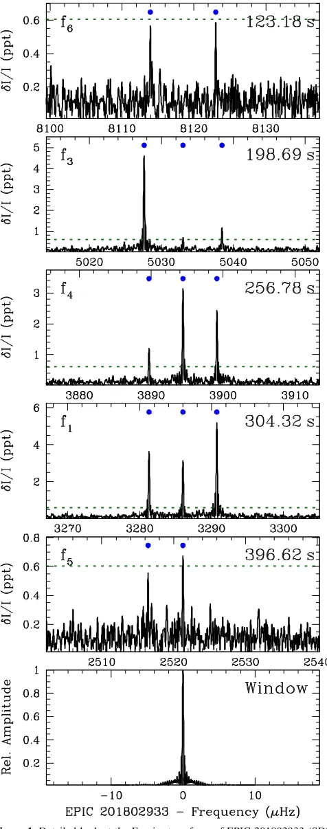
Figure1highlights a representative amplitude spectrum for a hot DAV: EPIC 201802933 (SDSS J1151+0525, Kp=17.7mag), observed for more than 77 days in K2Campaign 1. All Fourier transforms we compute were oversampled by a factor of 20, calculated from the software package PERIOD04 (Lenz & Breger 2005). We fit for and removed all instrumental artifacts arising from the long-cadence sampling rate, at integer multiples of roughly 566.48μHz(Gilliland et al.2010). All panels of Figure1 are on the same frequency scale, including the spectral window.
We computed a significance threshold for all DAVs from a shuffled simulation of the data, as described in Hermes et al.
(2015a). In summary, we keep the time sampling of our observed light curves but randomly shuffle the flux values to create 10,000 synthetic light curves, noting the highest peak in the Fourier transform for each synthetic data set. We set our 1%
(0.1%)False Alarm Probability(FAP)at the value for which 99%(99.9%)of these synthetic Fourier transforms do not have a peak exceeding that amplitude. We also list in Table 2 the value forfive times the average amplitude of the entire Fourier transform,5 Aá ñ.
For all DAVs, we adopt the 1% FAP as our significance threshold and produce a period list of observed pulsations, detailed in Table 5 in the Appendix. Our first set of uncertainties on the period, frequency, amplitude, and phase in Table5arise from a simultaneous nonlinear least-squaresfit to the significant peaks, calculated with PERIOD04. All light curves are barycentric corrected, and the phases in Table5are relative to the first mid-exposure time (T0) listed in Table 2. The frequencies of variability are not in the stellar rest frame, but many have high enough precision that they should eventually be corrected for the Doppler and gravitational redshift of the white dwarf(e.g., Davies et al.2014).
Importantly, we are able to identify the spherical degree(ℓ) of 87 out of 201 independent modes in these DAVs(more than 40%), based on common frequency patterns in the Fourier transforms, which in turn illuminates the rotation periods of these stellar remnants (see Section 7). When identified, we group in Table 5 each set of frequencies of the same radial order (k) and spherical degree (ℓ), and include the measured frequency splittings. We relax the significance threshold for a handful of modes that share common frequency splittings, which occasionally helps with identifying the correct azimuthal order (m) for the modes present. We have not attempted to quantify the exact radial orders of any of the pulsations here, but leave that to future asteroseismic analysis of these stars. 7
https://keplerscience.arc.nasa.gov/data/documentation/ KSCI-19080-002.pdf
8
All reduced light curves are available online athttp://www.k2wd.org.
4
4. Follow-up WHT and SOAR Spectroscopy
We complemented our space-based photometry of these 27 DAVs by determining their atmospheric parameters based on model-atmospherefits to follow-up spectroscopy obtained from two 4 m class, ground-based facilities. We detail these spectroscopic observations and their resultant fits in Table 3. Our spectra were obtained, reduced, andfit in a homogeneous way to minimize systematics.
DAVs in the original Keplermission field are at such high declination(d> +39deg)that they can only be observed from the northern hemisphere, so we used the Intermediate-dispersion Spectrograph and Imaging System(ISIS)instrument mounted on the 4.2 m William Herschel Telescope(WHT)on the island of La Palma for these five northern DAVs. Their spectra were taken with a 600 line mm−1 grating and cover roughly 3800–5100Å at roughly 2.0Å resolution using the blue arm of ISIS. A complete journal of observations for these
five DAVs is detailed in Greiss et al.(2016), and we only list in Table3the night for which most observations were obtained. AllK2fields lie along the ecliptic, so we obtained spectroscopy of all K2 DAVs with the Goodman spectrograph (Clemens et al. 2004) mounted on the 4.1 m Southern Astrophysical Research(SOAR) telescope on Cerro Pachón in Chile. Using a high-throughput 930 line mm−1grating, we adopted grating and camera angles(13 degrees and 24 degrees, respectively)that yield wavelength coverage from roughly 3600–5200Å. With 2×2 binning, our dispersion is 0.84Å pixel−1. To capture as much
flux as possible, we use a 3″ slit, so our spectral resolution is seeing limited, roughly 3Åin 1 0 seeing and roughly 4Åin 1 4 seeing.
For each DAV, we obtained a series of consecutive spectra covering at least two cycles of the highest-amplitude pulsation, as derived from theKeplerphotometry. We also made attempts to observe our targets at minimum airmass, which we list in Table3, along with the mean seeing during the observations, measured from the mean FWHM in the spatial direction of the two-dimensional spectra.
All of our spectra were debiased and flat-fielded using a quartz lamp, using standard STARLINK routines (Currie et al. 2014). They were optimally extracted (Horne 1986) using the software PAMELA. We then used MOLLY
(Marsh 1989) to wavelength calibrate, apply a heliocentric correction, and perform a final weighted average of the one-dimensional(1D)spectra. Weflux-calibrated each spectrum to a spectrophotometric standard observed using the same setup at a similar airmass, and used a scalar to normalize this final spectrum to the g magnitude from any of the SDSS, VST/ ATLAS, APASS, or KIS photometric surveys in order to correct itsfinal absoluteflux calibration.
We use the mean seeing to compute the spectral resolution, which informs the S/N per resolution element of the final spectra; the values listed in Table 3 were computed using a 100Åwide region of the continuum centered at 4600Å.
Wefit the six Balmer lines, Hβ–H9, of ourfinal 1D spectra to pure-hydrogen, 1D model atmospheres for white dwarfs. In short, the models employ the latest treatment of Stark broadening, as well as the ML2/α=0.8 prescription of the mixing-length theory. A full description of the models and
[image:6.612.48.286.51.654.2]fitting procedures is contained in Tremblay et al. (2011). For each individual DAV, the models were convolved to match the mean seeing during the observations.
Figure 1.Detailed look at the Fourier transform of EPIC 201802933(SDSS J1151+0525, Kp=17.7mag), a new DAV discovered with K2 and
representative of most of the hot DAVs analyzed here. The green dotted line shows the 1% FAP (see text). The K2 photometry features an exceptionally sharp spectral window(shown in the bottom panel), simplify-ing mode identification. All of the pulsations shown here are most simply interpreted as components of five different radial orders (k) of ℓ=1
dipole modes. The median frequency splitting of the five dipole modes is
f 4.7
d = μHz, which corresponds to a roughly 1.3 day rotation period(see Section7).
Table 3
Follow-up Spectroscopy of the First 27 Pulsating DA White Dwarfs Observed byKeplerandK2
KIC/EPIC g Facility, Night of Exp. Seeing Airm. S/N Teff-1D DTeff logg-1D Dlogg Teff-3D logg-3D MWD
(mag) (s) (″) Avg. (K) (K) (cgs) (cgs) (K) (cgs) (Me)
4357037 18.2 WHT, 2013 Jun 06 3×1200 0.9 1.07 77 12750 240 8.020 0.062 12650 8.013 0.62
4552982† 17.7 WHT, 2014 July 25 5×1200 0.7 1.06 76 11240 160 8.280 0.053 10950 8.113 0.67
7594781 18.1 WHT, 2014 July 25 6×1800 0.8 1.11 70 12040 210 8.170 0.059 11730 8.107 0.67
10132702 19.0 WHT, 2013 Jun 06 3×1500 0.9 1.06 70 12220 240 8.170 0.072 11940 8.123 0.68
11911480 18.0 WHT, 2013 Jun 07 3×1200 1.0 1.22 68 11880 190 8.020 0.061 11580 7.959 0.58
60017836 13.3 SOAR, 2016 Jul 14 5×30 2.1 1.11 210 11280 140 8.144 0.040 10980 7.995 0.60
201355934 17.8 SOAR, 2017 Apr 20 5×300 1.2 1.13 73 12050 170 8.016 0.047 11770 7.972 0.59
201719578 18.1 SOAR, 2017 Apr 14 8×300 1.4 1.22 62 11390 150 8.068 0.047 11070 7.941 0.57
201730811 17.1 SOAR, 2015 Jan 28 4×420 1.0 1.24 139 12600 170 7.964 0.043 12480 7.956 0.58
201802933 17.6 SOAR, 2016 Feb 14 3×360 1.4 1.23 75 12530 180 8.136 0.046 12330 8.114 0.68
201806008† 14.9 SOAR, 2016 Jun 22 7×180 1.1 1.29 161 11200 140 8.182 0.040 10910 8.019 0.61
206212611 17.3 SOAR, 2016 Jul 14 3×300 1.4 1.07 77 11120 150 8.170 0.048 10830 7.999 0.60
210397465 17.6 SOAR, 2016 Sep 01 5×300 1.8 1.27 50 11520 160 7.782 0.054 11200 7.713 0.45
211596649 18.9 SOAR, 2017 Feb 28 7×600 1.8 1.22 51 11890 180 7.967 0.057 11600 7.913 0.56
211629697† 18.3 SOAR, 2016 Dec 27 13×420 2.6 1.29 71 10890 150 7.950 0.060 10600 7.772 0.48
211914185 18.8 SOAR, 2017 Jan 25 9×600 2.0 1.38 61 13620 380 8.437 0.058 13590 8.434 0.88
211916160 18.9 SOAR, 2017 Apr 21 10×480 1.2 1.60 56 11820 170 8.027 0.053 11510 7.958 0.58
211926430 17.6 SOAR, 2016 Dec 27 11×420 2.2 1.30 98 11740 160 8.065 0.045 11420 7.982 0.59
228682478 18.2 SOAR, 2016 Jan 08 4×600 1.3 1.28 99 12340 170 8.226 0.046 12070 8.184 0.72
229227292† 16.6 SOAR, 2016 Feb 14 6×180 1.2 1.20 103 11530 150 8.146 0.042 11210 8.028 0.62
229228364† 17.8 SOAR, 2016 Jul 05 8×420 1.9 1.06 147 11330 140 8.172 0.043 11030 8.026 0.62
220204626 18.4 SOAR, 2016 Jul 05 7×420 1.7 1.22 74 11940 250 8.255 0.061 11620 8.173 0.71
220258806 16.2 SOAR, 2016 Jul 14 3×180 2.1 1.18 134 12890 200 8.093 0.047 12800 8.086 0.66
220347759 17.6 SOAR, 2016 Jul 05 5×300 1.5 1.32 81 12860 200 8.087 0.047 12770 8.080 0.66
220453225† 17.9 SOAR, 2016 Jul 05 7×300 1.6 1.49 72 11540 160 8.153 0.045 11220 8.035 0.62
229228478 16.9 SOAR, 2014 Oct 13 6×180 1.3 1.19 75 12610 180 7.935 0.045 12500 7.929 0.57
229228480 18.8 SOAR, 2016 Aug 07 7×600 1.0 1.17 65 12640 190 8.202 0.047 12450 8.181 0.72
References.We use a“†”symbol to mark thefirst six outbursting white dwarfs(Bell et al.2015,2016,2017; Hermes et al.2015b). (This table is available in machine-readable form.)
6
The
Astrophysical
Journal
Supplement
Series,
232:23
(
28pp
)
,
2017
October
Hermes
et
Figure 2.Averaged, normalized spectra for the 27 DAVs observed throughK2Campaign 8, overplotted with the best-fit atmospheric parameters detailed in Table3. We observed thefive DAVs from the originalKeplermission with the ISIS spectrograph on the 4.2 m William Herschel Telescope; all others were observed with the Goodman spectrograph on the 4.1 m SOAR telescope. Tremblay et al.(2011)describes the models andfitting procedures, which use ML2/a=0.8;atmospheric parameters have been corrected for the three-dimensional dependence of convection(Tremblay et al.2013).
The 1D effective temperatures and surface gravities found from thesefits are detailed in Table3; thefits are visualized in Figure 2. We add in quadrature systematic uncertainties of 1.2% on the effective temperature and 0.038 dex on the surface gravity (Liebert et al. 2005). We use the analytic functions based on the three-dimensional(3D)convection simulations of Tremblay et al. (2013) to correct these 1D values to 3D atmospheric parameters, which we list in Table3asTeff-3D and logg -3D. We adopt these 3D-corrected atmospheric parameters as our estimates of the effective temperature and surface gravity of our 27 DAVs here, and use them in concert with the white dwarf models of Fontaine et al. (2001; which have thick hydrogen layers and are uniformly mixed, 50% carbon and 50% oxygen cores)to estimate the overall mass of our DAVs. Our overall mass estimates do not change by more than the adopted uncertainties (0.04Me for all white dwarfs here) if we instead use the models of Renedo et al. (2010), which have more realistic carbon–oxygen profiles resulting from full evolutionary sequences.
Notably, two DAVs in our sample have line-of-sight dM companions, one of which strongly contaminates the Hβ line profiles. For this DAV(EPIC 220204626, SDSS J0111+0009), we omitted the Hβline from ourfits.
Ourfitting methodology differs slightly from that adopted by Greiss et al.(2016)in that wefit the averaged spectrum rather than each spectrum individually, so our reported parameters are slightly different from those reported there but are still within the 1σ uncertainties. However, we note that the values for KIC 4357037 (KIS J1917+3927) were misreported in Greiss et al.(2016)and are corrected here.
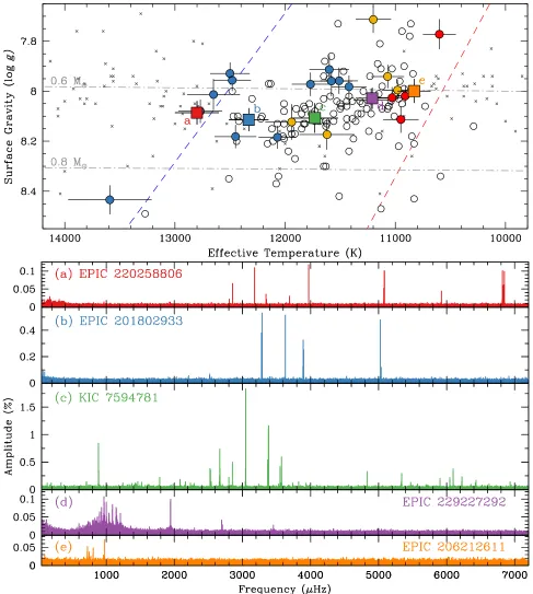
We put our spectroscopic effective temperatures and surface gravities in the context of the empirical DAV instability strip in Figure3; we show the empirical blue and red edges found by Tremblay et al.(2015). All atmospheric parameters, including literature DAVs and white dwarfs not observed to vary, were determined using the same 1D models using ML2/α=0.8, and all were corrected to account for the 3D dependence of convection. Since Kepler is often more sensitive to lower-amplitude pulsations than instruments from the ground, it appears the empirical blue edge of the instability strip may need to be adjusted by roughly 200 K to hotter temperatures, but we leave that discussion to future analyses.
We adopt in Figure 3 a color code that we will use throughout the manuscript. We mark in blue all DAVs with a weighted mean period(WMP)shorter than 600 s(as described in more detail in Section6), which cluster at the hotter(blue) half of the instability strip. We mark in gold all DAVs with a WMP exceeding 600 s. Finally, we mark in red the first six outbursting DAVs(Bell et al.2017), all of which we mark in Table3with a “†”symbol. These outbursting DAVs are also all cooler than 11,300 K and exhibit stochastic, large-amplitude
flux excursions we call outbursts.
Outbursts in the coolest DAVs werefirst discovered in the long-baseline monitoring of the Kepler spacecraft (Bell et al. 2015)and confirmed in a second DAV observed in K2 Campaign 1 (Hermes et al. 2015b). A detailed discussion of this interesting new phenomenon is outside the scope of this paper, but we previously demonstrated that outbursts affect
(and may be affected by)pulsations(Hermes et al.2015b). Interestingly, there are threeK2pulsating white dwarfs near or even cooler than thefirst six outbursting DAVs. One of these
Figure 3.DAVs withKeplerdata in the context of the empirical DAV instability strip, demarcated with the blue and red dashed lines most recently updated by Tremblay et al.(2015). We mark all DAVs with weighted mean pulsation periods shorter than 600 s in blue and those greater than 600 s in gold(see Section6). Cool DAVs that show outbursts are marked in red(see Section6). Known DAVs from ground-based observations are shown with open circles, and DAs not observed to vary to higher than 4 ppt are marked with gray crosses(Gianninas et al.2011; Tremblay et al.2011). All atmospheric parameters were analyzed with the same models, using ML2/α=0.8, and corrected for the 3D dependence of convection(Tremblay et al.2013). Dashed–dotted gray lines show the cooling tracks for 0.6Meand
0.8Mewhite dwarfs(Fontaine et al.2001).
8
three is GD1212, which only has nine days of observations, so the limits on a lack of outbursts are not robust. GD1212 was re-observed byK2for more than 75 days in Campaign 12 and will be analyzed in a future publication. We will discuss our insights into the evolution of white dwarfs through the DAV instability strip fromK2in Section6.
5. A Dichotomy of Mode Line Widths
Long-baseline Kepler photometry has opened an unprece-dented window into the frequency and amplitude stability of DAVs. From early observations of thefirst DAV observed with Kepler, we noticed broad bands of power in the Fourier transform. Rather than just a small number of peaks, we saw a large number of peaks under a broad envelope; the envelope was significantly wider than the sharp spectral windows (Bell et al. 2015). We saw similarly broad power bands in another cool DAV, GD 1212, observed during an engineering test run forK2(Hermes et al.2014). The broadly distributed power was reminiscent of the power spectra of stochastically driven
oscillations in the Sun or other solar-like oscillators(Chaplin & Miglio 2013). However, as noted in Bell et al. (2015), white dwarfs have a sound-crossing time orders of magnitude shorter than their observed pulsation periods, so these broad line widths cannot be related to stochastic driving.
Additionally, it became clear that not all white dwarfs with long-baseline, space-based observations showed such broad line widths. For example, we observed multiple DAVs with hotter effective temperatures and shorter-period pulsations that were completely coherent, within the uncertainties, over several months of Kepler observations (Greiss et al. 2014; Hermes et al.2015a).
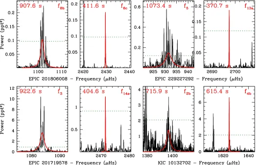
[image:10.612.46.571.52.390.2]Within the larger sample of thefirst 27 DAVs, we noticed an emergent pattern: a dichotomy of mode line widths, even within the same star, delineated almost entirely by the pulsation period. The shorter-period modes appear stable in phase, producing narrow peaks in the Fourier transform, while the longer-period modes are phase unstable, spreading their power over a broad band in the Fourier transform. To quantify this
Figure 4.Detailed portions of the Fourier transforms of four DAVs observed withK2showing that pulsations with periods exceeding roughly 800 s(frequencies
<1250μHz)have power broadly distributed outside the spectral window of theKeplerobservations. For every DAV, wefit a Lorentzian to each independent mode, as described in Section5. In the top left, we show two modes in EPIC 201806008(PG 1149+058):f8b, likely them=0 component of anℓ=2mode centered at 907.6 s, has power broadly distributed, with HWHM=0.868μHz, whereasf6c, them= +1component of theℓ=1mode centered at 412.40 s, has a sharp peak with HWHM=0.056μHz. Similarly, in the top-right panels, we show two modes in EPIC 229227292(ATLAS J1342−0735): the band of power centered at 1073.44 s, which has HWHM=1.632μHz, is significantly broader than them= -1component of theℓ=1mode centered at 370.05 s. The bottom-left panels show a similar behavior in EPIC 201719578(WD 1119+042): the 922.60 s mode in the same star has an HWHM of 0.836μHz, whereas the 404.60 s mode has an HWHM of 0.045μHz. Finally, we show KIC 10132702(KIS J1913+4709)in the bottom-right panel, where the 715.86 s mode has an HWHM of 1.632μHz, whereas the 615.44 s mode has an HWHM of 0.104μHz. Thex-axis(frequency)scales are identical for each star. The bestfits for each mode are detailed in Table5and overplotted here; the HWHM of the Lorentzianfits to all 27 DAVs are shown in Figure5.
behavior, we fit Lorentzian envelopes to every significant pulsation period and compare the period determined to the half-width at half-maximum (HWHM, γ) of the Lorentzian fits. Motivated by Toutain & Appourchaux (1994), we fit each thicket of peaks in the power spectrum (the square of the Fourier transform)with the function
A
B
Power , 1
2
0 2 2
g
n n g
=
- + +
( ) ( )
whereArepresents the Lorentzian height,γis the HWHM,n0is
the central frequency of the peak, andBrepresents a DC offset for the background, which we hold fixed for all modes in the same star as the median power of the entire power spectrum. We onlyfit the region within 5μHz to each side of the highest-amplitude peak within each band of power; this highest peak defines our initial guess for the central frequency, and we use an initial guess for the HWHM of 0.2μHz, roughly twice our typical frequency resolution.
We illustrate the nature of the dichotomy of the mode line widths in Figure4. Here we show, for four different DAVs in our sample, two independent modes within the same star that are well-separated in period. In each case, the shorter-period modes have line widths roughly matching the spectral window of the observations, with HWHM 0.1μHz. All DAVs in Figure4were observed by theKeplerspacecraft for more than 78 days with a duty cycle exceeding 91%. We observe that modes exceeding roughly 800 s (with frequencies below
roughly 1250μHz)have much broader HWHM, often exceed-ing 1μHz.
These broad bands of power are most likely representative of a single mode that is unstable in phase, reminiscent of a damped harmonic oscillator. For example, in the top-left panels of Figure4, we show two modes in EPIC 201806008(PG 1149
+058), the second outbursting DAV discovered (Hermes et al. 2015b). The modef6cis the m= +1component of the
ℓ=1mode centered at 412.40 s; the two other components are seen at a slightly lower frequency(we discuss this splitting in the context of rotation in Section 7). The HWHM of f6c is consistent with the spectral window:g=0.056μHz. At much lower frequency, we identify the modef8bas the likelym=0 component of anℓ=2mode centered at 907.58 s. Its power is much more broadly distributed, with g=0.868 μHz, too narrow to encompass other normal modes of different degrees or radial orders, but much broader than the spectral window.
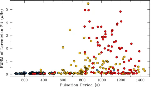
We extend this Lorentzian analysis of mode line widths to the entire sample of 27 DAVs in Figure 5, which shows the period and HWHM computed for every Lorentzianfit to all 225 significant pulsations (we exclude all nonlinear combination frequencies from Figure 5; see Section 6). We performed the same experiment by fitting Gaussians to each peak and obtained a nearly identical distribution, so our choice of function does not significantly alter our results.
[image:11.612.66.550.52.332.2]We see a sharp increase in HWHM at roughly 800 s, indicating that modes with relatively high radial order(k>15 for ℓ=1 modes)are not phase coherent, exhibiting behavior
Figure 5.Half-width at half-maximum(HWHM)of Lorentzian functionsfit to all significant peaks in the power spectra of the 27 DAVs observed throughK2
Campaign 8 by theKeplerspace telescope; our procedure is described in Section5. We use the same color classification as in Figure3, where blue denotes objects with WMP<600 s, gold with WMP>600 s, and red those with outbursts(see Section6). We excluded any nonlinear combination frequencies in this analysis. We see a sharp increase in HWHM at roughly 800 s, indicating that modes with relatively high radial order(k>15forℓ=1modes)are not coherent in phase, similar in behavior to stochastically excited pulsators. We save a discussion of the possible physical mechanisms behind this phenomenon for a future work(M. H. Montgomery et al. 2017, in preparation).
10
similar to stochastically excited pulsators, although we do not believe the mode instability is related to stochastic driving.
One possibility is that the broad line widths arise from a process that has disrupted the phase coherence of the modes. In analogy with stochastically driven modes, we relate the observed mode line width (HWHM) to its lifetime (τ) via the relationt=2 (pg)(Chaplin et al.2009). Doing so for the longer-period modes (g>1μHz), wefind mode lifetimes of order several days to weeks. This is comparable to the damping rates we expect for the roughly 1000 sℓ=1modes of typical pulsating white dwarfs (Goldreich & Wu 1999). We will explore the possible physical mechanisms to explain these broad line widths in a future publication (M. H. Montgomery et al. 2017, in preparation).
Determining a pulsation period to use for the asteroseis-mology of the coolest DAVs with the longest-period modes is different from that for hot DAVs with narrow pulsation peaks that are determined via a linear least-squares fit and cleanly prewhitened. Therefore, for all modes with fitted HWHM exceeding 0.2μHz, we do not include their linear least-squares fits in Table 5, and instead only include the periods and amplitudes as determined from the Lorentzian fits in Table 5, with the period uncertainties computed from the HWHM.
6. Characteristics of the DAV Instability Strip
Pulsations in DAVs are excited by the“convective driving” mechanism, which is intimately tied to the surface hydrogen partial-ionization zone that develops as a white dwarf cools below roughly 13,000 K (Brickhill 1991; Wu & Goldreich 1999). Driving is strongest for pulsations with periods nearest
to roughly 25 times the thermal timescale at the base of the convection zone(Goldreich & Wu1999).
By the time white dwarfs reach the DAV instability strip, their evolution is dominated by secular cooling. As they cool, the surface convection zone deepens, driving longer-period pulsations (e.g., Van Grootel et al. 2013). These ensemble characteristics of the DAV instability strip, especially the lengthening of periods with cooler effective temperature, have been considered for decades (e.g., Clemens 1994) and were most recently summarized observationally by Mukadam et al.(2006).
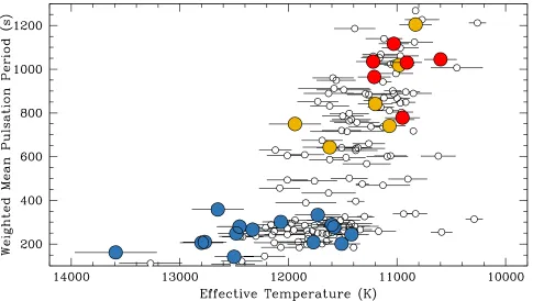
The most common way to visualize the increasing mode periods as DAVs cool is to compute the WMP of the significant pulsations(Clemens1993). The WMP is linearly weighted by the amplitude of each mode, such thatWMP= åiP Ai i åiAi, wherePiandAiare the period and amplitude, respectively, of each significant independent pulsation detected (excluding nonlinear combination frequencies). We show the WMPs of all 27 DAVs observed by Kepler and K2 so far in Figure 6, in addition to the WMP and temperatures of previously known DAVs with atmospheric parameters determined in the same way by Gianninas et al.(2011)and Tremblay et al.(2011).
[image:12.612.66.551.50.324.2]Extensive coverage by theKeplerspace telescope affords an even more nuanced exploration of the DAV instability strip. With our follow-up spectroscopic characterization of the first 27 DAVs observed withKeplerandK2, we can effectively put the evolutionary state of our pulsating white dwarfs into greater context. Figure7 highlightsfive DAVs that are representative of the five different stages of evolution through the DAV instability strip, including color-coded Fourier transforms of each representative object. These data reveal important trends in the period and amplitude evolution of DAVs through the
Figure 6.Following Clemens(1993), we plot the effective temperature vs. the weighted mean pulsation period(WMP)of each DAV analyzed here, using the same color classification used in Figure3. We also show with white circles the 114 known DAVs from the literature with spectroscopy analyzed in the same way, also plotted in Figure3.
instability strip. Since there are likely mass-dependent effects, we describe this sequence for DAVs near the meanfield white dwarf mass of 0.62Me, in order of hottest to coolest DAVs.
[image:13.612.63.550.50.593.2](a)DAVs begin pulsating at the blue edge of the instability strip with low-k (1< <k 6) ℓ=1, 2 modes from roughly 100–300 s and relatively low amplitudes (∼1 ppt). We
Figure 7.Top panel shows the same information as Figure3but color codesfive representative stars in our sample to highlight the various phases of DAV cooling illuminated byKeplerobservations so far, especially the pulsation period and amplitude evolution. In order of decreasing effective temperature, we highlight(a)EPIC 220258806(SDSS J0106+0145),(b)EPIC 201802933(SDSS J1151+0525),(c)KIC 7594781(KIS J1908+4316),(d)EPIC 229227292(ATLAS J1342−0735), and
(e)EPIC 206212611(SDSS J2220−0933). Fourier transforms of each are shown below with the same order and color coding, with amplitudes adjusted to reflect the targetflux fractions found in Table2. DAVs begin pulsating at the blue edge of the instability strip(a)with low-k(1< <k 4)ℓ=1, 2modes from roughly 100–300 s and relatively low amplitudes(∼1 ppt). As they cool,(b)their convection zones deepen, driving longer-period(lower-frequency)pulsations with growing amplitudes. DAVs in the middle of the instability strip(c)have high-amplitude modes and the greatest number of nonlinear combination frequencies. As they cool further,(d)it appears common for DAVs to undergo aperiodic, sporadic outbursts; these DAVs tend to have many low-frequency modes excited in addition to one or several shorter-period, stable pulsations. Finally, a handful of DAVs have effective temperatures cooler than the outbursting DAVs but do not experience large-scale
flux excursions(e); these coolest DAVs have the longest-period pulsations with relatively low amplitudes.
12
highlight in red in Figure 7 the hot (12,800 K) white dwarf EPIC 220258806 (SDSS J0106+0145) that appears to fall at the blue edge of the instability strip. This DAV has stable pulsations ranging from 116.28–356.14 s (WMP=206.0 s), most of which are clearly identified as both ℓ=1and ℓ=2 modes (see Table 5), although no modes have amplitudes in excess of roughly 1 ppt. The hottest DAVs in our sample have relatively low-amplitude modes. For example, the hottest DAV currently known is EPIC 211914185 (SDSS J0837+1856), which has just two relatively low-amplitude (1–3 ppt) dipole modes centered at 109.15 and 190.45 s (Hermes et al.2017c). An example of a well-studied blue-edge DAV in this phase of evolution from ground-based observations is G226−29(Kepler et al.1995).
(b)As DAVs cool by a few hundred degrees from the blue edge, they retain relatively short-period pulsations but their observed amplitudes increase. For example, the 12,330 K EPIC 201802933(SDSS J1151+0525)has amplitudes up to roughly 5 ppt with modes ranging from 123.11 to 396.62 s
(WMP=266.2 s). These low-k modes are expected to have extremely long mode lifetimes (Goldreich & Wu 1999), and most modes in these hot DAVs with mode periods shorter than 400 s appear coherent in phase. A well-known example of this phase of DAV evolution is G117-B15A(Robinson et al.1995; Kepler et al.2000).
(c)After DAVs cool by nearly 1000 K from the blue edge of the instability strip, their dominant pulsations exceed 300 s. DAVs in the middle of the instability strip tend to have very high-amplitude modes and the greatest number of nonlinear combination frequencies. For example, KIC 7594781 (KIS J1908+4316) is an 11,730 K white dwarf with the largest number of pulsation frequencies presented in our sample
(WMP=333.3 s). However, fewer than 10 of these frequen-cies of variability actually arise from unstable stellar oscilla-tions—the rest are nonlinear combination frequencies (e.g., peaks corresponding to f1+f2 or 2f1), which arise from distortions of a linear pulsation signal caused by the changing convection zone of a DAV(Brickhill1992; Montgomery2005). These are not independent modes but rather artifacts of some nonlinear distortion in the outer layers of the star (Hermes et al.2013).
Objects in the middle of the DAV instability strip represent a transition from hot, stable pulsations to cool DAVs with oscillations that are observed to change in frequency and/or amplitude on relatively short timescales. G29−38 is a prominent, long-studied example of a DAV representative of this phase in the middle of the instability strip (Kleinman et al.1998).
(d)Keplerobservations have now confirmed what appears to be a new phase in the evolution of DAVs as they approach the cool edge of the instability strip: aperiodic outbursts that increase the mean stellarflux by a few to 15%, last several hours, and recur sporadically on a timescale of days. Outbursts were first discovered in the originalKepler mission(Bell et al.2015)and quickly confirmed in K2 (Hermes et al. 2015b). Observational properties of the first six outbursting DAVs are detailed in Bell et al.(2017). Aside from many long-period pulsations, almost all of the outbursting DAVs observed byKepleralso show at least one and sometimes multiple shorter-period modes. Figure 7 highlights the Fourier transform of the 11,210 K outbursting DAV EPIC 229227292(ATLAS J1342−0735), which is dominated by
pulsations from 827.7 to 1323.6 s (WMP=964.5 s) but also shows significant periods centered around 514.1 s, 370.0 s, and 288.9 s (see Table 5). From the brightest outbursting DAV observed so far(PG 1149+058), we saw strong evidence that the pulsations respond to the outbursts(Hermes et al.2015b).
(e)Finally, a handful of DAVs have effective temperatures as cool or cooler than the outbursting DAVs but do not experience large-scale flux excursions, suggesting that not all DAVs outburst at the cool edge of the instability strip. The coolest DAVs tend to have the longest-period pulsations with relatively low amplitudes. We highlight in Figure 7 the star EPIC 206212611 (SDSS J2220−0933), which is one of the coolest DAVs known, at 10,830 K. We do not detect any outbursts to a limit of 5.5%, following the methodology outlined in Bell et al. (2016). This DAV has modes from 1023.4 to 1381.2 s (WMP=1204.4 s), all at relatively low amplitudes below 1 ppt.
7. Rotation Rates
The oscillations observed in white dwarfs are non-radial g-modes, which can be decomposed into spherical harmonics. Pulsations can thus be represented by three quantum numbers: the radial order (k, often expressed as n in other fields of asteroseismology), representing the number of radial nodes; the spherical degree (ℓ), representing the number of nodal lines expressed at the surface of the star; and the azimuthal order(m), representing the number of nodal lines in longitude at the surface of the star, ranging from-ℓ toℓ.
Due to the strong geometric cancellation of higher-ℓmodes, we typically observeℓ=1, 2modes in white dwarfs. Rotation causes a lifting of degeneracy in the pulsation frequencies, causing a mode to separate into2ℓ+1components inm(Unno et al. 1989). If all multiplets are present, this can result in triplets(forℓ=1modes)and quintuplets(forℓ=2modes)in the presence of slow rotation. This is corroborated by the many DAVs we observed with Kepler that show triplets and quintuplets of peaks evenly spaced in frequency: an exquisite example is the hot DBV PG 0112+104(Hermes et al.2017b). Observationally (and in contrast to solar-like oscillations), white dwarf pulsations do not partition mode energy equally into the various m components, such that the amplitudes of different m components for a given k ℓ, are not necessarily symmetric.
Still, we can use the clear patterns of frequency spacing in the Fourier transforms of our DAVs to say something about the rotation of these stellar remnants, summarized in Figure8. This task is often complex from the ground due to diurnal aliasing, but the extended Kepler observations significantly simplifies mode identification and affords us the opportunity to probe internal rotation for 20 of the 27 DAVs we present here. For example, Figure1shows thefive dipole(ℓ=1)modes in EPIC 201802933 (SDSS J1151+0525) identified from their split-tings. Evidence for splittings in other DAVs analyzed here can be found in Section8.
To first order, the observed pulsation frequency splittings
(dn) are related to the stellar rotation frequency (Ω) by the relation
m 1 Ck ℓ, , 2
dn= ( - )W ( )
where Ck ℓ, represents the effect of the Coriolis force on the
pulsations, as formulated by Ledoux(1951). For high-kmodes that approach the asymptotic, mode-independent limit forℓ=1 modes, Ck,10.50. However, the low-k (especially k<10) modes found in hot DAVs can suffer from strong mode-trapping effects that also significantly alterCk ℓ, (e.g., Brassard
et al.1992). Theoretical DAV models in, for example, Romero et al.(2012), predictCk,1values typically ranging from roughly
0.45 to 0.49, with exceptions down toCk,1~0.35for strongly trapped modes.
For the 20 DAVs here for which we have identified modes, all have at least one and many have multiple sets of ℓ=1 modes; the full catalog of asteroseismic rotation rates for white dwarfs is detailed in Table 4. To provide the best model-independent estimates for the rotation periods of the newly identified DAVs here, we compute the median frequency splitting of all identifiedℓ=1modes(dnℓ=1), which we list in
Table 4. We then hold fixed Ck,1=0.47 and use dnℓ=1 to
estimate the DAV rotation period. We put these new DAV rotation periods in the context of all other white dwarfs with measured rotation periods from asteroseismology compiled by Kawaler (2015) in Figure 8. Kepler and K2 have more than doubled the number of white dwarfs for which we have measured internal rotation from pulsations.
We note that it is necessary to perform a complete asteroseismic analysis in order to estimate the best values for
Ck ℓ, for the pulsation modes presented here. This also affords us
the opportunity to significantly improve constraints on the rotation period; the choice of Ck ℓ, for each mode dominates
the uncertainty on the overall rotation period measured from
the frequency splittings, since mode trapping is very common. Given our method of uniformly adopting Ck,1=0.47, we estimate that each rotation period has a systematic uncertainty of roughly 10%, though we note thatCk ℓ, cannot exceed 0.50.
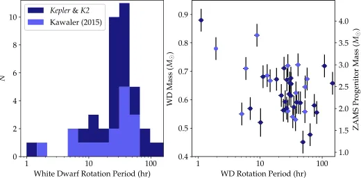
Importantly, because we measured the atmospheric para-meters of all DAVs observed withKeplerso far, we have for thefirst time a large enough sample to determine how rotation periods in white dwarfs differ as a function of the overall white dwarf mass. We see in Figure 8 suggestions of a trend of decreasing rotation period with increasing white dwarf mass. We also include on the right axis estimates for the ZAMS progenitor mass, calculated from the cluster-calibrated white dwarf initial-to-final-mass relation of Cummings et al. (2016) for progenitor stars with masses below 4.0Me.
Afirst-order linearfit to the white dwarf mass–rotation plot in the right panel of Figure 8 yields an estimate of the final white dwarf rotation rate as a function of progenitor mass:
Prot=((2.360.14)-MZAMS) (0.00240.0031), where
Prot is the final rotation period expressed in hours and MZAMS
is the ZAMS progenitor mass in solar masses. This linear trend is not yet statistically significant; we are actively seeking more white dwarfs with masses exceeding 0.72Me (which likely arise from>3.0MeZAMS progenitors)to improve estimates of this relationship.
[image:15.612.47.567.53.309.2]The mass distribution of white dwarfs with rotation periods measured from pulsations is very similar to the mass distribution of field white dwarfs determined by Tremblay et al.(2016). If we restrict our analysis to only white dwarfs within 1σ of the mean mass and standard deviation of field white dwarfs(i.e., nearly 70% of allfield white dwarfs), we are
Figure 8.We compare asteroseismically determined rotation periods for all known pulsating white dwarfs, detailed in Table4. All white dwarfs presented here appear to be isolated stars, so these rotation periods should be representative of the endpoints of single-star evolution; we excluded the only known close binary(a WD+dM in a 6.9 hr orbit), EPIC 201730811(SDSS J1136+0409, Hermes et al.2015a). The left histogram shares the color coding of the right panel, which compares white dwarf rotation as a function of mass. Estimates of the ZAMS progenitor masses for each white dwarf are listed on the right axis. Notably, EPIC 211914185(SDSS J0837+1856)is more massive(0.88±0.03Me)and rotates faster(1.13±0.02 hr)than any other pulsating white dwarf(Hermes et al.2017c); we see evidence for a
link between high mass and fast rotation, but require additional massive white dwarfs to confirm this trend.
14
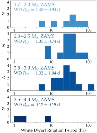
left with 34 pulsating white dwarfs with masses from 0.51 to 0.73Me which have a mean rotation period of 35 hr with a standard deviation of 28 hr (35±28 hr). The mean rotation period is essentially the same if we break the subsample into progenitor ZAMS masses spanning 1.7–2.0Me(35±23 hr), 2.0–2.5Me(32±18 hr), and 2.5–3.0Me(32±25 hr). How-ever, the small sample of three massive white dwarfs, which evolved from 3.5 to 4.0Me progenitors, appears to rotate significantly faster, at 4.0±3.5 hr. This is visualized in Figure9.
The originalKeplermission yielded exceptional insight into the rotational evolution of stars at most phases of stellar
[image:16.612.46.568.75.527.2]evolution(Aerts2015), and now we can providefinal boundary conditions on the question of internal angular momentum evolution in isolated stars. For example,Keplerdata have been especially effective at illuminating differential rotation and angular momentum evolution in 1.0–2.0Me first-ascent red giants(e.g., Mosser et al.2012), where it was found that their cores are rotating roughly 10 times faster than their envelopes. Still, this is an order of magnitude slower than expected after accounting for all hypothesized angular momentum transport processes (e.g., Marques et al. 2013; Cantiello et al. 2014). Moving farther along the giant branch,Kepler has shown that 2.2–2.9Me core-helium-burning secondary clump giants do
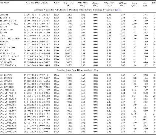
Table 4
Rotation Rates of Isolated White Dwarfs Determined via Asteroseismology
Star Name R.A. and Decl.(J2000) Class Teff−3D WD Mass DMWD Prog. Mass DMProg. dnℓ=1 Prot Ref.
(K) (Me) (Me) (Me) (Me) (μHz) (hr)
Literature Values for All Classes of Pulsating White Dwarfs Compiled by Kawaler(2015)
Ross 548 01 36 13.58−11 20 32.7 DAV 12300 0.62 0.04 2.36 0.47 L 37.8 1
HL Tau 76 04 18 56.63+27 17 48.5 DAV 11470 0.56 0.04 1.93 0.44 L 52.8 2
HS 0507+0434 05 10 13.94+04 38 38.4 DAV 12010 0.72 0.04 3.00 0.52 3.6 40.9 3 KUV11370+4222 11 39 41.42+42 05 18.7 DAV 11940 0.71 0.04 2.92 0.51 25.0 5.9 4
GD 154 13 09 57.69+35 09 47.1 DAV 11120 0.65 0.04 2.49 0.48 2.8 53.3 5
LP 133−144 13 51 20.24+54 57 42.6 DAV 12150 0.59 0.04 2.13 0.45 L 41.8 6
GD 165 14 24 39.14+09 17 14.0 DAV 12220 0.67 0.04 2.68 0.50 L 57.3 1
L19-2 14 33 07.60−81 20 14.5 DAV 12070 0.69 0.04 2.75 0.50 13.0 13.0 7
SDSS J1612+0830 16 12 18.08+08 30 28.1 DAV 11810 0.78 0.04 3.50 0.55 75.6 1.9 8
G226-29 16 48 25.64+59 03 22.7 DAV 12510 0.83 0.04 3.68 0.57 L 8.9 9
G185-32 19 37 13.68+27 43 18.7 DAV 12470 0.67 0.04 2.64 0.49 L 14.5 10
PG 0122+200 01 25 22.52+20 17 56.8 DOV 80000 0.53 0.04 1.75 0.42 3.7 37.2 11
NGC 1501 04 06 59.39+60 55 14.4 DOV 134000 0.56 0.04 1.94 0.44 L 28.0 12
PG 1159−035 12 01 45.97−03 45 40.6 DOV 140000 0.54 0.04 1.81 0.43 L 33.6 13 RX J2117.1+3412 21 17 08.28+34 12 27.5 DOV 170000 0.72 0.04 2.98 0.52 L 28.0 14 PG 2131+066 21 34 08.23+06 50 57.4 DOV 95000 0.55 0.04 1.88 0.43 L 5.1 15 KIC 8626021 19 29 04.69+44 47 09.7 DBV 30000 0.59 0.04 2.10 0.45 3.3 44.6 16 EPIC 220670436 01 14 37.66+10 41 04.8 DBV 31300 0.52 0.04 1.68 0.42 15.4 10.2 17
Rotation Rates from DAVs Analyzed Here
KIC 4357037 19 17 19.20+39 27 19.1 DAV 12650 0.62 0.04 2.30 0.47 6.7 22.0 0 KIC 4552982 19 16 43.83+39 38 49.7 DAV 10950 0.67 0.04 2.67 0.50 8.0 18.4 18 KIC 7594781 19 08 35.88+43 16 42.4 DAV 11730 0.67 0.04 2.66 0.49 5.5 26.8 0 KIC 10132702 19 13 40.89+47 09 31.3 DAV 11940 0.68 0.04 2.73 0.50 13.2 11.2 0 KIC 11911480 19 20 24.90+50 17 21.3 DAV 11580 0.58 0.04 2.07 0.45 1.97 74.7 19 EPIC 60017836 23 38 50.74−07 41 19.9 DAV 10980 0.57 0.04 2.00 0.44 21.2 6.9 0 EPIC 201719578 11 22 21.10+03 58 22.4 DAV 11070 0.57 0.04 2.01 0.44 5.5 26.8 0 EPIC 201730811 11 36 55.16+04 09 52.8 DAV 12480 0.58 0.04 2.08 0.45 56.7 2.6 20 EPIC 201802933 11 51 26.15+05 25 12.9 DAV 12330 0.68 0.04 2.69 0.50 4.7 31.3 0 EPIC 201806008 11 51 54.20+05 28 39.8 DAV 10910 0.61 0.04 2.29 0.47 4.7 31.3 0 EPIC 210397465 03 58 24.23+13 24 30.8 DAV 11200 0.45 0.04 1.23 0.38 3.0 49.1 0 EPIC 211596649 08 32 03.98+14 29 42.4 DAV 11600 0.56 0.04 1.91 0.44 1.8 81.8 0 EPIC 211629697 08 40 54.14+14 57 09.0 DAV 10600 0.48 0.04 1.40 0.40 2.3 64.0 0 EPIC 211914185 08 37 02.16+18 56 13.4 DAV 13590 0.88 0.04 4.02 0.60 131.6 1.1 21 EPIC 211926430 09 00 41.08+19 07 14.4 DAV 11420 0.59 0.04 2.16 0.46 5.8 25.4 0 EPIC 228682478 08 40 27.84+13 20 10.0 DAV 12070 0.72 0.04 2.97 0.52 1.4 109.1 0 EPIC 229227292 13 42 11.62−07 35 40.1 DAV 11210 0.62 0.04 2.33 0.47 5.0 29.4 0 EPIC 220204626 01 11 23.89+00 09 35.2 DAV 11620 0.71 0.04 2.92 0.51 6.1 24.3 0 EPIC 220258806 01 06 37.03+01 45 03.0 DAV 12800 0.66 0.04 2.58 0.49 4.9 30.0 0 EPIC 220347759 00 51 24.25+03 39 03.8 DAV 12770 0.66 0.04 2.56 0.49 4.7 31.7 0
References.(0)This work;(1)Giammichele et al.(2016);(2)Dolez et al.(2006);(3)Fu et al.(2013);(4)Su et al.(2014);(5)Pfeiffer et al.(1996);(6)Bognár et al.
(2016);(7)Bradley(2001);(8)Castanheira et al.(2013);(9)Kepler et al.(1995);(10)Pech & Vauclair(2006);(11)Fu et al.(2007);(12)Bond et al.(1996);(13) Charpinet et al.(2009);(14)Vauclair et al.(2002);(15)Kawaler et al.(1995);(16)Østensen et al.(2011);(17)Hermes et al.(2017b);(18)Bell et al.(2015);(19) Greiss et al.(2014);(20)Hermes et al.(2015a)—excluded from Figure8since the white dwarf is in a close, post-common-envelope binary;(21)Hermes et al.
(2017c).
not have as much radial differential rotation and have cores rotating at roughly 30–100 days(e.g., Deheuvels et al.2015).
For decades, we have known that white dwarfs have relatively slow rotation, given that their surface rotation velocities usually do not exceed upper limits of 15 km s−1, corresponding to periods longer than several hours (Koester et al. 1998). This is surprising: if we completely conserve the angular momentum of a 3.0Me main-sequence star with an initial rotation period of 10 hr, its white dwarf remnant would be rotating faster than a few minutes (Kawaler 2004). We establish here that the majority of isolated descendants of 1.7–3.0Me ZAMS progenitors rotate at 1.5 days, with a narrow dispersion between 0.5 and 2.2 days at the conclusion of their evolution. We note that we are sensitive to rotation periods longer than 15 days given our frequency resolution, but
the longest rotation period we measure is 109.1 hr (roughly 4.5 days)in EPIC 228682478.
8. Notes on Individual Objects
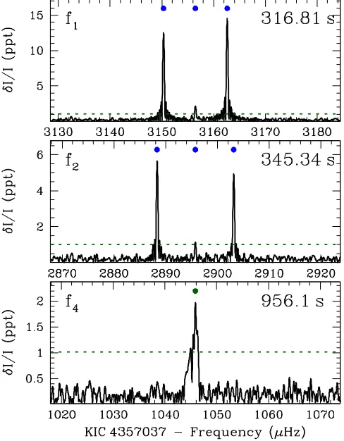
KIC 4357037(KIS J1917+3927): With“only”36.3 days of nearly uninterrupted Kepler observations, this is one of our shortest data sets, but still the data reveal seven independent pulsations,five of which we identify asℓ=1modes; we show in Figure 10 the two highest-amplitude modes, f1 and f2. As noted in Section4, the atmospheric parameters for this object were misreported in Greiss et al.(2016), but are corrected here andfindTeff=12,650 K. Most periods we observe are in line
[image:17.612.137.471.51.508.2]with such a hot DAV, with the identifiedℓ=1modes spanning 214.40–396.70 s. However, there are several long-period
Figure 9.Rotation rates of pulsating, apparently isolated white dwarfs as a function of initial stellar mass, using the cluster-calibrated IFMR from Cummings et al.
(2016). The 34 pulsating white dwarfs with masses from 0.51 to 0.73Me(which descended from roughly 1.7 to 3.0MeZAMS stars)all have a mean rotation period
of roughly 35 hr regardless of binning, but more massive white dwarfs(>0.75Me, which descended from>3.5MeZAMS stars)appear to rotate systematically
faster.
16
modes that do not appear to be nonlinear difference frequencies, at 549.72 and 956.11 s. The latter mode at 956.11 s (bottom panel of Figure 10) is significantly broader than the spectral window, with HWHM=0.318μHz, suggest-ing that it is an independent mode in the star, given its position in Figure 5. It is at a much longer period than typically observed in such a hot DAV, posing an interesting question of how it is excited at the same time as other modes with three times shorter periods.
KIC 4552982 (KIS J1916+3938): This was the first DAV discovered in the original Kepler mission field and has the longest pseudo-continuous light curve of any pulsating white dwarf ever recorded, spanning more than 1.5 years. Our analysis here is focused on the HWHM of the modes present, and thus only includes roughly three months of data from Q12, to remain consistent with the frequency resolution of the other DAVs analyzed here. A more detailed light curve analysis, including discussion of the mean period spacing and results from Lorentzianfits to the fullKeplerdata set, can be found in Bell et al. (2015). The triplet atf1 remains the only mode we have identified in this DAV; the large amplitude of this coherent mode atf1drives down the WMP of this DAV to 750.4 s, which we report from the period list of Bell et al.(2015). Our rotation rate differs slightly from that reported by Bell et al.(2015)since we adopt a lower assumed value forCk ℓ,.
KIC 7594781(KIS J1908+4316): This DAV has a relatively short data set, with just 31.8 days of observations in Q16.2. We identify three modes in the star asℓ=1with a median splitting of 5.5μHz, two of which are shown in Figure11, suggesting a rotation period of 26.8 hr. Such a rotation rate would yieldℓ=2 splittings of roughly 8.6μHz, so we suggest thatf1may be an
[image:18.612.322.563.50.361.2]ℓ=2 mode, although the data are not definitive. As with KIC 4357037, there is a much longer period, highly broadened mode, here at 1129.19 s. Interestingly, this mode,f3, combines with many other modes in the star to give rise to most of the 14 nonlinear combination frequencies present. When f3 combines with other modes, its unique line width is reproduced; for this reason, although we could not identify any suitable combinations, we caution that f4 may not be an independent mode in the star but could possibly be a combination frequency of f3 in some way given the shape of f4. Interestingly, f3 is relatively stable in amplitude but changing rapidly in frequency. Its frequency in thefirst five days of data is relatively stable at 885.243±0.057μHz (7.08±0.32 ppt), but its power in the lastfive days ofKeplerdata less than 27 days later had almost completely moved to 888.285±0.067μHz (6.14±0.32 ppt). There is still much to be learned about the causes of short-term frequency, amplitude, and phase instability in white dwarf pulsations from further analysis of thisKeplerdata—nonlinear mode coupling appears to be the only way to explain how white dwarf pulsations can change character so rapidly (e.g., Zong et al.2016).
Figure 10.Highest-amplitude modes in KIC 4357037(KIS J1917+3927),f1
and f2 (ℓ=1modes marked with blue dots), illuminate the median ℓ=1
splitting of 6.8μHz, corresponding to a 22.0 hr rotation period. We could not identify the longest-period mode also present in this star at 956.11 s
[image:18.612.47.291.54.367.2](unidentified modes marked with green dots), which has a considerably broader line width than the shorter-period modes.