The effect of the point spread function on sub-pixel mapping
1
2
Qunming Wang a, Peter M. Atkinson a,b,c,*
3
4
a
Lancaster Environment Centre, Lancaster University, Lancaster LA1 4YQ, UK
5
b
Geography and Environment, University of Southampton, Highfield, Southampton SO17 1BJ, UK
6
c
School of Geography, Archaeology and Palaeoecology, Queen's University Belfast, BT7 1NN, Northern Ireland, UK
7
8
*Corresponding author
9
E-mail: [email protected]
10
11
Abstract: Sub-pixel mapping (SPM) is a process for predicting spatially the land cover classes within mixed
12
pixels. In existing SPM methods, the effect of point spread function (PSF) has seldom been considered. In this
13
paper, a generic SPM method is developed to consider the PSF effect in SPM and, thereby, to increase
14
prediction accuracy. We first demonstrate that the spectral unmixing predictions (i.e., coarse land cover
15
proportions used as input for SPM) are a convolution of not only sub-pixels within the coarse pixel, but also
16
sub-pixels from neighboring coarse pixels. Based on this finding, a new SPM method based on optimization is
17
developed which recognizes the optimal solution as the one that when convolved with the PSF, is the same as
18
the input coarse land cover proportion. Experimental results on three separate datasets show that the SPM
19
accuracy can be increased by considering the PSF effect.
20
21
Keywords: Land cover mapping, downscaling, sub-pixel mapping (SPM), super-resolution mapping, point
22
spread function (PSF), Hopfield neural network (HNN).
23
24
1. Introduction 26
27
Mixed pixels are inevitable in remote sensing images and have brought great challenges in land cover
28
mapping. The spectral unmixing technique has been studied for decades to estimate the proportions of land
29
cover classes within mixed pixels (Bioucas-Dias et al., 2012; Heinz & Chang, 2001; Keshava & Mustard,
30
2002). The proportions are at the same spatial resolution as the input images and cannot inform the spatial
31
distribution of classes within mixed pixels. To further estimate the spatial distribution of land cover, sub-pixel
32
mapping (SPM) was developed as a post-processing analysis of spectral unmixing outputs. SPM divides mixed
33
pixels to sub-pixels and predicts their class attributes under the coherence constraint from prior spectral
34
unmixing predictions (i.e., coarse land cover class proportions). SPM transforms the conventional pixel-level
35
classification to a finer spatial resolution hard classification (Atkinson, 1997), which can provide more explicit
36
thematic information (e.g., the boundaries between land cover classes can be characterized by more pixels).
37
In recent decades, various SPM approaches have been developed. As a post-processing step of spectral
38
unmixing, two main groups of SPM approaches can be identified. The first group considers the relation
39
between sub-pixels and solutions are always produced based on defined objectives. Based on the assumption of
40
spatial dependence, the objective can be determined empirically as maximizing the spatial attraction between
41
sub-pixels (Makido & Shortridge, 2007), maximizing the Moran’s I (Makido et al., 2007) or minimizing the
42
perimeter of the area for each class (Villa et al., 2011). Based on prior knowledge, the objective can also be
43
matching prior patterns extracted from training images, such as characterized by the semivariogram (Tatem et
44
al., 2002), two-point histogram (Atkinson, 2008) or landscape structure (Lin et al., 2011). The SPM solutions
45
of this type of methods are achieved based on optimization, including the Hopfield neural network (HNN)
46
(Ling et al., 2010; Muad & Foody, 2012; Nguyen et al., 2011; Tatem et al., 2001), pixel swapping algorithm
47
(PSA) (Atkinson, 2005; Shen et al., 2009; Xu & Huang, 2014), maximum a posteriori method (Zhong et al.,
48
2015), genetic algorithm (Li et al., 2015; Mertens et al., 2003; Tong et al., 2016), and particle swarm
49
optimization (PSO) (Wang et al., 2012). Several iterations are involved for this group of SPM methods and,
thus, a relatively long computing time may be required. The second group of SPM methods considers the
51
relation between sub-pixels and neighboring pixels. The coarse class proportions within each pixel are used
52
directly to characterize the relation between it and sub-pixels and calculate the fine spatial resolution
53
proportions for sub-pixels. Under the coherence constraint, the sub-pixel classes are determined by comparing
54
the fine spatial resolution proportions. As the coarse proportions are fixed for a given pixel, iterations (as in the
55
first method type) are not necessarily involved and SPM solutions can be produced more quickly. Methods
56
falling into this type include sub-pixel/pixel spatial attraction model (SPSAM) (Mahmood et al., 2013; Mertens
57
et al., 2006; Xu et al., 2014), back-propagation neural network-based algorithm (Gu et al., 2008; Zhang et al.,
58
2008), learning-based algorithm (Zhang et al., 2014), kriging (Verhoeye & Wulf, 2002; Boucher & Kyriakidis,
59
2006) and radial basis function (RBF) (Wang et al., 2014a) interpolation. They can also be summarized as the
60
soft-then-hard SPM (STHSPM) algorithms, a concept proposed in our previous work (Wang et al., 2014b;
61
Chen et al., 2015). In addition, to reduce the uncertainty introduced by spectral unmixing, some SPM methods
62
that do not rely absolutely on coarse proportions were developed, including spatial-spectral methods (Ardila et
63
al., 2011; Kasetkasem et al., 2005; Li et al., 2014; Tolpekin & Stein, 2009), spatial regularization (Ling et al.,
64
2014; Zhang et al., 2015) and contouring methods (Foody & Doan, 2007; Ge et al., 2014; Su et al., 2012).
65
In remote sensing images, the point spread function (PSF) effect exists ubiquitously. It means that the signal
66
for a given pixel is a weighted combination of contributions from within the pixel and also contributions from
67
neighboring pixels (Townshend et al., 2000; Van der Meer, 2012). The PSF can brighten dark objects and
68
darken bright objects observed from the surface (Huang et al., 2002). It results in a fundamental limit on the
69
amount of information that remote sensing images can contain (Manslow & Nixon, 2002). The PSF is a
70
two-dimensional function accounting for both the across-track and along-track directions (Campagnolo &
71
Montano, 2014; Radoux et al., 2016). The PSF effect is caused mainly by the optics of the instrument, the
72
detector and electronics, atmospheric effects, and image resampling (Huang et al., 2002; Schowengerdt, 1997).
73
The PSF effect may not be an important issue for homogeneous regions, but it is crucial for heterogeneous
74
landscapes dominated by mixed pixels. To the best of our knowledge, very few SPM methods have considered
the PSF effect in downscaling. For example, in most of the existing SPM methods, the coherence constraint
76
from class proportions is satisfied simply by fixing the number of sub-pixels for each class within a single
77
coarse pixel (i.e., the ideal square wave PSF is considered). The number of sub-pixels to be allocated to a class
78
within a coarse pixel is calculated as the product of the coarse class proportion within the coarse pixel and the
79
square of the zoom factor. Due to the PSF effect, however, the coarse proportions estimated by spectral
80
unmixing are actually a function, in part, of the neighboring coarse pixels. The uncertainty in coarse
81
proportions is propagated to the post-SPM process where the coarse proportions contaminated by neighboring
82
coarse pixels are used as the coherence constraint. There is, therefore, a great need for an approach accounting
83
for the PSF effect in SPM to increase the prediction accuracy.
84
There are two plausible solutions to cope with the PSF effect in SPM. One is to consider the PSF effect in the
85
pre-spectral unmixing process and to estimate more reliable coarse proportions from observed multispectral
86
images. Based on the more reliable predictions, the PSF need not be considered in SPM (i.e., the ideal square
87
wave PSF can be considered in SPM, as in existing SPM approaches). However, spectral unmixing is an
88
ill-posed inverse problem. It is more complicated when part of the neighboring coarse pixels (i.e., neighboring
89
sub-pixels) are involved as this technique is generally performed at the pixel resolution. Currently, it is
90
challenging to account for the PSF in spectral unmixing and obtain reliable proportions. The alternative
91
solution, considered here, is to model the PSF effect in the SPM process, based on the proportions
92
contaminated by neighboring coarse pixels. This strategy is more feasible as SPM is conducted at the sub-pixel
93
scale and contributions from neighboring sub-pixels in PSF can be straightforwardly modeled.
94
In this paper, to increase the SPM accuracy, the PSF effect is considered directly in the SPM process. Most
95
SPM methods need to first calculate the number of sub-pixels for each class within each coarse pixel. Based on
96
these fixed numbers, the sub-pixel classes are then predicted. This is not a problem for the ideal square wave
97
PSF, as mentioned earlier. When considering the non-ideal PSF, however, the coarse proportions are a
98
convolution of the sub-pixel class values in a larger local window, rather than the single coarse pixel in the
99
ideal square-wave PSF. In this case, the number of sub-pixels for each class in each coarse pixel cannot be
determined using only the single coarse proportion (i.e., product of the coarse proportion and the square of the
101
zoom factor, as in existing SPM methods), and it actually cannot be calculated explicitly. In this case, SPM
102
methods such as the STHSPM algorithms are not suitable choices. A plausible solution to this issue is to
103
convolve the fine spatial resolution SPM realization with the PSF and compare the estimated proportion with
104
the actual coarse proportion, and use the error to guide further updating of the current realization. The
105
iteration-based HNN is a method of this type. Therefore, in this paper, the HNN is used to reduce the
106
uncertainty in SPM introduced by the PSF effect.
107
The remainder of this paper is organized into four sections. Section 2 first introduces the mechanism of the
108
PSF effect in SPM and then the details of the proposed strategy for considering the PSF in SPM. The
109
experimental results for three groups of datasets are provided in Section 3 for validation of the proposed
110
method. Section 4 further discusses the proposed SPM method, followed by a conclusion in Section 5.
111
112
113
2. Methods 114
115
2.1. The PSF effect in SPM
116
This section will illustrate the PSF effect in SPM and demonstrate that the coarse proportions in SPM are a
117
convolution of the sub-pixel class values in a local window centered at the coarse pixel. Let SV be the spectrum
118
of coarse pixel V, Rk be the spectrum of class endmember k (k=1, 2, …, K, where K is the number of land
119
cover classes), and F Vk( ) be the proportion of class k in pixel V. Based on the classical linear spectral mixture
120
model (Bioucas-Dias et al., 2012; Heinz & Chang, 2001; Keshava & Mustard, 2002), the spectrum of each
121
coarse pixel is a linear combination of the spectrum of endmembers, where the weights are determined as the
122
class proportions within the coarse pixel. That is
123
1
( )
K
V k k
k
F V
S R . (1)
Due to the PSF effect in remote sensing images, Eq. (2) holds
125
V vhV
S S (2)
126
where Sv is the spectrum of sub-pixel v, hV is the PSF and * is the convolution operator. For sub-pixel v, its
127
spectrum Sv can be characterized as
128
1
( )
K
v k k
k
I v
S R (3)
129
in which I vk( ) is a class indicator as follows
130
1, if sub-pixel belongs to class ( )0, otherwise
k
v k
I v . (4)
131
By substituting Eq. (3) into Eq. (2), we have
132
1 1
( ) = ( )
K K
V k k V k k V
k k
I v h I v h
S R R . (5)
133
The comparison between Eq. (1) and Eq. (5) leads to
134
( ) ( )
k k V
F V I v h . (6)
135
Let z be the zoom factor, that is, each coarse pixel is divided into z by z sub-pixels. As shown in the one
136
dimensional illustration in Fig. 1, when the PSF takes the ideal square wave filter in Eq. (7)
137
2 1
, if ( , ) ( , ) ( , )
0, otherwise
V
i j V i j
h i j z
(7)
138
where (i, j) is the spatial location of the sub-pixel and V i j( , ) is the spatial extent of the coarse pixel V
139
containing the sub-pixel at (i, j). Further, the convolution in Eq. (6) can be simplified as
140
, 1 2
( ) ( )
z
k ij i j k
I v F V
z
. (8)141
In Eq. (8), all sub-pixels vij are located within coarse pixel V. This means that based on the assumption of an
142
ideal square wave PSF, the coarse class proportion estimated from the linear spectral mixture model in Eq. (1)
is viewed as the average of all sub-pixel class indictors within the pixel. This is the common case considered in
144
most SPM methods.
145
146
pixel PSF
sub-pixel Ideal square PSF
[image:7.612.150.460.127.234.2]147
Fig. 1 A one dimensional illustration of the PSF in SPM. Based on the real PSF, the coarse pixel value (or coarse class proportion) 148
should be a convolution of the sub-pixel values (or sub-pixel class indicators) located within the local window centered at the coarse 149
pixel, rather than only within the single coarse pixel (as assumed in the ideal square wave PSF). 150
151
In reality, the PSF is different to the ideal square wave filter. The spatial coverage of hV is generally larger
152
than a coarse pixel size, but is finite, as shown in Fig. 1. For example, the PSF can be the Gaussian filter, which
153
is used widely in remote sensing (Campagnolo & Montano, 2014; Huang et al., 2002; Manslow & Nixon, 2002;
154
Townshend et al., 2000; Van der Meer, 2012; Wenny et al., 2015)
155
2 2
2 2
1
exp , if ( , ) ( , )
( , ) 2 2
0, otherwise
V
i j
i j V i j
h i j
(9)
156
where is the standard deviation (width of the Gaussian PSF) and V i j( , ) is the spatial extent of the local
157
window centered at coarse pixel V (V covers the sub-pixel at (i, j)), see Fig. 1. Thus, any sub-pixel v involved in
158
the calculations in Eq. (2) and Eq. (6) falls within a wider spatial coverage V i j( , ), rather than only within
159
( , )
V i j . This means that based on the linear spectral mixture model in Eq. (1), the estimated coarse class
160
proportions within each coarse pixel are actually a convolution of the sub-pixels in the local window centered
161
at the coarse pixel, rather than only the sub-pixels within the coarse pixel (i.e., not the case in Eq. (8)).
162
163
2.2. Enhancing SPM by considering the PSF effect
165
In conventional SPM, the number of sub-pixels for each class needs to be determined in advance, which is
166
used as a coherence constraint in the mapping process. Let N Vk( ) be the number of sub-pixels for class k in
167
pixel V, which is usually calculated as
168
2
( ) round ( )
k k
N V F V z . (10)
169
From Section 2.1, it is concluded that in reality the estimated coarse proportions are contaminated by their
170
neighboring pixels due to the PSF effect (see Eq. (6)). Therefore, it is generally incorrect to use Eq. (10) for the
171
coherence constraint in SPM, unless the correct land cover proportions (i.e., not contaminated by neighbors)
172
can be produced. As can be seen from Eq. (5), even when the endmember set Rk and PSF hV are known
173
perfectly, it is not trivial to determine the correct proportions. This is because the coarse proportions can
174
sometimes be functions of neighboring sub-pixels, as can be seen from Eq. (6) and Fig. 1. In this case where
175
sub-pixels are involved, spectral unmixing becomes challenging, as unmixing is carried out at the pixel
176
resolution and cannot account for proportions at the sub-pixel resolution. Townshend et al. (2000) and Huang
177
et al. (2002) proposed an interesting deconvolution method to reduce the impact of the PSF in coarse
178
proportion predictions. This method was developed at the pixel resolution, which quantifies the contributions
179
from neighbors in units of coarse pixels. That is, it treats all sub-pixels in a surrounding coarse pixel equally
180
and assumes a uniform contribution to the center coarse pixel. According to Fig. 1, however, sub-pixels in the
181
surrounding coarse pixel have a different spatial distance to the center coarse pixel and thus, should have
182
different contributions to the center coarse proportion (e.g., some sub-pixels even have no contribution).
183
In this paper, the coarse proportions contaminated by pixel neighbors are directly considered in SPM. As
184
( )
k
N V cannot be calculated explicitly, conventional SPM methods such as the STHSPM algorithms cannot be
185
used. Guided by the mechanism in Eq. (6), the ideal SPM solution should be the one that when convolved with
186
the PSF, is the same as the coarse proportion. Alternatively, an optimization-based SPM method is employed in
187
this paper, where the convolution of the current SPM realization is compared with the contaminated coarse
proportions for updating SPM predictions iteratively. The HNN is a method suitable for this task and is used for
189
accounting for the PSF in SPM. The HNN has been used widely in SPM, appreciating its highly satisfactory
190
performance (Ling et al., 2010; Muad & Foody, 2012; Nguyen et al., 2011; Tatem et al., 2001). It considers
191
each sub-pixel as a neuron and works by minimizing an energy function composed of a goal and a coherence
192
constraint term. The HNN accounting for the PSF effect is introduced below.
193
Suppose (k, i, j) is a neuron for sub-pixel at location (i, j) and is on the network layer representing land cover
194
class k, and qkij is its output. If qkij is 1, it means that the sub-pixel at (i, j) is belongs to class k, and if qkij is 0,
195
the sub-pixel does not belong to class k. Using the HNN, the outputs are update iteratively for each sub-pixel.
196
The output qkij is a function of the input signal ukij
197
1
1 tanh 2
kij kij
q u (11)
198
where determines the steepness of the function. The input ukij for the t-th iteration is updated by
199
kij
kij kij
du t
u t dt u dt
dt
(12)
200
in which dt is a time step. The second term on the right hand side of Eq. (12) is the energy change of the
201
neuron and is described as
202
kij kij
kij
du t dE
dt dq . (13)
203
In Eq. (13), E represents the network energy function and is described as
204
1 1kij 2 2kij 3 kij 4 kij
k i j
E
w G w G w P w M (14)205
where w1, w2, w3 and w4 are four weights, G1 and G2 are two spatial clustering functions characterizing
206
spatial dependence, P is the proportion constraint and M is the multi-class constraint (Ling et al., 2010; Nguyen
207
et al., 2011). Accordingly, the energy change of the neuron for sub-pixel at (i, j) in Eq. (13) is determined by
208
1 2 3 4
1 2
kij kij kij kij kij
kij kij kij kij kij
dE dG dG dP dM
w w w w
dq dq dq dq dq . (15)
The first two terms of the right hand side of Eq. (15) are calculated as
210
1 1
1 1
1 1 1
1 tanh 0.5 1
2 8
i i
kij
kbc kij kij
b i c j kij
dG
q q q
dq
(16) 211 1 1 1 12 1 1
1 tanh 0.5
2 8
i i
kij
kbc kij kij
b i c j kij
dG
q q q
dq
. (17)
212
If the average output of the surrounding neurons is larger than 0.5, the function G1 increases the neuron output
213
to approach 1 to increase the spatial correlation between neighboring sub-pixels. Otherwise, if the average
214
output of the surrounding neurons is less than 0.5, the function G2 decreases the neuron output to 0.
215
The multi-class constraint means that for any sub-pixel, the sum of neuron outputs for all K classes should be
216
equal to 1, thus
217 1 1 K kij nij n kij dM q dq
. (18) 218Considering the PSF effect, the proportion constraint for class k is expressed as
219
( ) ( )
kij
k ij k ij
kij dP
L V F V
dq (19)
220
where Vij is the coarse pixel that sub-pixel at (i, j) falls within, F Vk( ij) is the target coarse proportion of class k
221
in the pixel (i.e., spectral unmixing predictions), and L Vk( ij) is the coarse proportion estimated as convolution 222
of the current SPM realization. Based on the mechanism in Eq. (6), L Vk( ij) is calculated as
223
0 0( , ) ( , ) 1
( ) 1 tanh 0.5 * 2
1
1 tanh 0.5 ( , )
2
k ij k V
k V x y
x y V i j
L V q h
q h x i y j d d
(20) 224in which V i j( , ) is defined in the same way as that in Eq. (9) and ( ,i0 j0) is the spatial location of the center of
225
coarse pixel Vij. The tanh function is used in Eq. (20) to ensure that if the neuron output qk is above 0.5, it is
226
counted as an output of 1 (i.e., belongs to class k) for the coarse proportion calculation; If qk is below 0.5, it is
not counted for class k instead. This ensures that the neuron output exceeds 0.5 in order to be counted within the
228
calculations for each class.
229
In Eq. (19), the target coarse proportion F Vk( ij) is used to examine the current SPM realization. The
230
convolution of the final SPM prediction should be the same as the target coarse proportion. Specifically, if the
231
convolution of the current SPM realization, L Vk( ij), is larger than the target proportion F Vk( ij), a positive
232
gradient is produced and the energy is reduced to decrease the neuron output (see Eq. (12) and Eq. (13)) to cope
233
with this overestimation issue. On the contrary, if L Vk( ij) is smaller than F Vk( ij), a negative gradient is
234
produced and the neuron output is increased correspondingly to cope with underestimation. After a number of
235
iterations (usually over 1000), L Vk( ij) will approach F Vk( ij), suggesting that the convolution of the final
236
prediction is almost identical to the target coarse proportion contaminated by the PSF effect. In this way, the
237
PSF effect in SPM is considered and a more reliable sub-pixel class distribution can be reproduced. It should be
238
noted that the proposed HNN-based SPM method accounting for the PSF is suitable for any PSF. Its
239
implementation is not affected by the specific form of PSF. Once the PSF of the sensor is available or estimated,
240
it can be used readily in the proposed method, as shown in Eq. (20).
241
As suggested in Tatem et al. (2001), for the HNN, the network will converge to similar energy minima given
242
any initialization and the network will converge to an accurate prediction in fewer iterations if a
243
proportion-constrained initialization is used. This scheme was employed in the proposed method for faster
244
convergence of the optimization. According to Eq. (6), in the estimated coarse proportions images, if a pixel is
245
presented as a pure pixel (e.g., belongs entirely to class k), all sub-pixels in the local window centered at the
246
coarse pixel must belong to class k. Thus, for any pure pixel in the coarse proportion image for class k, we
247
directly initialize the neuron outputs of all sub-pixels within it as 1 for class k and 0 for other classes. These
248
values are fixed and not changed in the optimization process. For mixed pixels, random initialization (between
249
0 and 1) was applied.
250
3. Experiments 252
253
Experiments were carried out on three groups of synthetic datasets, including a dataset with six different
254
targets, a land cover map with multiple classes, and a multispectral image. They were used to test the
255
performance of SPM methods on different typical shapes in Section 3.1, multiple classes in Section 3.2 and the
256
case involving realistic unmixing in Section 3.3. As mentioned earlier, the proposed method is suitable for any
257
PSF. The estimation of the PSF of sensors is still an open problem, and uncertainty unavoidably exists in the
258
process. It is beyond the scope of this paper to estimate the PSF. Alternatively, to concentrate solely on the
259
performance of SPM, all coarse data for the three groups of datasets were produced by convolving the available
260
fine spatial resolution data, using a Gaussian PSF shown in Eq. (9), which is a widely used PSF (Campagnolo
261
& Montano, 2014; Huang et al., 2002; Manslow & Nixon, 2002; Townshend et al., 2000; Van der Meer, 2012; 262
Wenny et al., 2015). The width of the PSF was set to half of the coarse pixel size. Based on this strategy, the
263
fine spatial resolution data are known perfectly and can be used as a reference for evaluation. All SPM results
264
were evaluated both visually and quantitatively. For quantitative evaluation, the classification accuracy of each
265
class and the overall accuracy (OA) in terms of the percentage of correctly classified pixels were used. In
266
addition, to emphasize the improvement of the proposed method over the other methods, an index called the
267
reduction in remaining error (RRE) (Wang et al., 2015) was also used, as calculated below
268
1 0
1 RE RE
RRE 100%
RE
(21)
269
where RE and 1 RE are the remaining errors of OA (i.e., 100%-OA) for the benchmark method and the 0
270
proposed method, respectively.
271
272
3.1. Experiment on the six targets
273
In this experiment, six binary images (pixel value 1 for white target while 0 for black background) with
274
different targets were used for validation. They represent typical, basic shapes in nature. All six images have a
spatial size of 56 by 56 pixels and were marked as T1-T6, as shown in Fig. 1(a). Each image was degraded with
276
a Gaussian PSF and a zoom factor of 7, generating coarse images with 8 by 8 pixels, as shown in Fig. 1(b). The
277
coarse images are exactly the simulated coarse proportions of the white targets in each image.
278
Fig. 3 shows the relation between the PSF-convolved coarse proportions and actual proportions for the six
279
white targets. The actual proportions were generated by averaging the sub-pixel class indicators within each
280
coarse pixel. As observed from the plots, the proportions are very different to the actual values due to the PSF
281
effect. For example, in all six plots, many proportions should be 0 (i.e., pure background pixel and no target
282
pixel in the coarse pixel), but were actually calculated as values larger than 0 (i.e., mixed pixel). The reason is
283
that although no target pixels exist in a coarse pixel, they may be located in neighboring pixels. According to
284
Eq. (6), these neighboring pixels will contaminate the center pixel which will then not be recognized as a pure
285
background pixel. The accuracies of the coarse proportions were quantified in terms of root mean square error
286
(RMSE) and correlation coefficient (CC), as listed in Table 1. The uncertainty in the PSF-convolved coarse
287
proportions motivates the development of SPM methods considering the PSF effect.
288
289
Table 1 Accuracy of the coarse proportion images for the six targets 290
T1 T2 T3 T4 T5 T6
RMSE 0.0421 0.0602 0.0671 0.0707 0.0924 0.0972
CC 0.9949 0.9902 0.9820 0.9868 0.9677 0.9668
291
The SPM results of the HNN without PSF (that is, with ideal PSF) and with the Gaussian PSF are shown in
292
Fig. 2(c) and Fig. 2(d), respectively. It is seen clearly that by considering the PSF effect, more accurate SPM
293
results can be produced. In the results for target T1-T3, the proposed method produces more compact shapes
294
that are closer to the reference. For T4 and T5, the proposed method produces a straighter line than the HNN
295
without PSF. In T6, the more complex boundaries of the target are reproduced by the proposed method.
296
297
298
(a) (b) (c) (d) 300
301
302
303
304
305
[image:14.612.131.484.48.648.2]306
Fig. 2 SPM results of six targets. (a) Reference images (56 by 56 pixels). (b) Coarse images (8 by 8 pixels) produced by degrading (a) 307
with a Gaussian PSF and a factor of 7. (c) SPM results produced using the HNN without PSF (or with ideal PSF). (d) SPM results 308
produced using the proposed HNN with the Gaussian PSF. Lines 1-6 are results for T1-T6. 309
311
Fig. 3 Relation between the actual proportions (for white target) and proportions (for white target) contaminated due to the PSF effect 312
for the six binary images (z=7). From left to right are results for T1-T6. 313
314
Quantitative assessment in terms of OA (accuracy statistics for both target and background in each image) is
315
listed in Table 2. As mentioned earlier, for pure pixels, all sub-pixels within them are simply assigned to the
316
same class to which the pure pixel belongs. As suggested by the existing literature (Mertens et al., 2003), this
317
copy process will only increase the SPM accuracy statistics without providing any useful information on the
318
actual performance of the SPM methods. Hence, for the synthetic coarse images, we did not consider the pure
319
pixels in the accuracy statistics. The quantitative evaluation was conducted for two different zoom factors, z=4
320
and 7. As observed from the table, the HNN with PSF produces a larger OA than the HNN without PSF.
321
Moreover, the advantage tends to be more obvious when a larger zoom factor is involved. More precisely, for
322
T2 and T5, using the proposed method, the accuracy gains are below 1% for z=4, but increase to be above 2%
323
for z=7. For T6, the proposed method considering the PSF increases the OA by 1.4% for z=4 and 4.7% for z=7.
324
In addition, all RREs are generally large (over 10%) and some even reach over 60%, suggesting that the
325
accuracy increase is obvious.
326
327
Table 2 OA (%) of HNN-based SPM with two different schemes for the six binary images 328
T1 T2 T3 T4 T5 T6
z=4
no PSF 99.34 98.72 98.00 98.44 98.30 96.66
PSF 99.34 99.52 99.26 99.19 98.67 98.08
RRE 0% 62.50% 63.00% 48.08% 21.76% 42.51%
z=7
no PSF 99.41 97.31 97.89 97.34 94.48 90.53
PSF 99.46 99.26 98.16 97.91 97.51 95.18
RRE 8.47% 72.49% 12.80% 21.43% 54.89% 49.10%
329
0 0.5 1
0 0.5 1 Actual proportions E st im a te d p ro p o rt io n s
0 0.5 1
0 0.5 1 Actual proportions E st im a te d p ro p o rt io n s
0 0.5 1
0 0.5 1 Actual proportions E st im a te d p ro p o rt io n s
0 0.5 1
0 0.5 1 Actual proportions E st im a te d p ro p o rt io n s
0 0.5 1
0 0.5 1 Actual proportions E st im a te d p ro p o rt io n s
0 0.5 1
[image:15.612.113.501.587.716.2]330
[image:16.612.81.534.50.205.2]331
Fig. 4 The accuracy of the two SPM methods in relation to the width of the PSF (in units of coarse pixel, which was produced by 332
degrading Fig. 2(a) with a factor of 7). From left to right are results for T1, T2 and T5, respectively. 333
334
The influence of the width of the Gaussian PSF was also analyzed, as shown in Fig. 4. The fine spatial
335
resolution T1, T2 and T5 images were degraded with a factor of 7. Three PSF sizes, 0.5, 0.75 and 1 coarse
336
pixels, were considered for each target. Three observations can be made from the results in Fig. 4. First, for all
337
PSF sizes, the consideration of the PSF effect can lead to consistently larger OA than that produced without the
338
PSF. Second, the accuracy of SPM methods decreases as the width of the PSF increases, no matter whether the
339
PSF is accounted for or not. This is because more neighboring sub-pixels are involved in the convolution
340
process and the SPM problem becomes more complex as the width increases. Third, as the width increases, the
341
advantage of considering the PSF is more obvious.
342
343
3.2.Experiment on the land cover map with multiple classes
344
A land cover map produced from an aerial photograph covering an area in Bath, UK was used in this
345
experiment, as shown in Fig. 5. The image has a spatial resolution of 0.6 m, and a spatial size of 360 by 360
346
pixels. Four classes were identified in the land cover map, including roads, trees, buildings and grass. The map
347
was degraded with a factor of 8 and a Gaussian PSF, generating four proportion images at a spatial resolution
348
of 4.8 m. The relation between the simulated coarse proportions and actual proportions is shown in the plots in
349
Fig. 6. Table 3 lists the accuracies of the proportions. Similarly to the observation in Fig. 3 and Table 1, the two
350
types of proportions are very different due to the PSF effect.
351
OA
(%)
OA
(%)
OA
(%)
(a) (b) 352
353
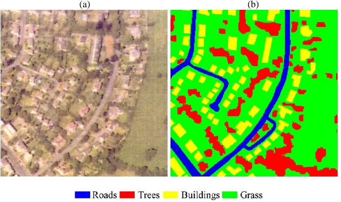
[image:17.612.134.481.52.258.2]354
Fig. 5 The land cover map. (a) Original aerial photograph. (b) Reference map drawn manually from (a). 355
356
[image:17.612.93.518.320.423.2]357
Fig. 6 Relation between the actual proportions and proportions contaminated due to the PSF effect for the land cover map (z=8). From 358
left to right are results for roads, trees, buildings and grass. 359
360
Table 3 Accuracy of the coarse proportion images for the land cover map 361
Roads Trees Buildings Grass Mean
RMSE 0.0440 0.0576 0.0591 0.0924 0.0633
CC 0.9866 0.9867 0.9844 0.9792 0.9842
362
The proposed method is not only compared to the original HNN method, but also to several typical SPM
363
methods. As mentioned in the Introduction, there are mainly two families of SPM methods for post-processing
364
of spectral unmixing. One is the method considering the relation between sub-pixels and neighboring pixels,
365
while the other considers the relation between sub-pixels. The SPSAM (Mertens et al., 2006) and RBF (Wang
366
et al., 2014a) methods were selected for the former and PSA (Makido et al., 2007) was selected for the latter.
367
0 0.5 1
0 0.5 1 Actual proportions E st im a te d p ro p o rt io n s
0 0.5 1
0 0.5 1 Actual proportions E st im a te d p ro p o rt io n s
0 0.5 1
0 0.5 1 Actual proportions E st im a te d p ro p o rt io n s
0 0.5 1
[image:17.612.173.440.527.582.2]For these three benchmark methods, the number of sub-pixels for each class needs to be determined first. The
368
numbers were calculated according to Eq. (10), where uncertainty from the PSF effect exists in the coarse
369
proportions. The SPM results of all five methods are presented in Fig. 7.
370
371
(a) (b) (c) 372
373
(d) (e) (f) 374
375
[image:18.612.50.565.153.549.2]376
Fig. 7 SPM results of the land cover map with 360 by 360 pixels (z=8). (a) SPSAM (no PSF). (b) RBF (no PSF). (c) PSA (no PSF). (d) 377
HNN (no PSF). (e) The proposed HNN with PSF. (f) Reference. 378
379
Due to the uncertainty in the coarse proportions, the SPM predictions of SPSAM and RBF contain a number
380
of jagged artifacts and the boundaries of classes are rough. Although PSA is able to enhance the performance
381
and produce a more compact result, the class boundaries are still not smooth and some noisy pixels exist.
382
Different from the three methods, the original HNN method produces a cleaner result and the class boundaries
are smoother, although the PSF is not considered. The reason is that the HNN is not absolutely slavish to the
384
coarse proportions, and can remove isolated pixels and produce a compact result by the two spatial clustering
385
functions G1 and G2 (see Eq. (16) and Eq. (17)). However, there are some needle-like artifacts for restoration
386
of roads and trees in the HNN result. Using the proposed method accounting for the PSF effect, the result is
387
more accurate than the original HNN without the PSF method. For example, the prediction of the roads by the
388
proposed method is smoother, and needle-like artifacts are removed. The result of the proposed method is the
389
closest to the reference in Fig. 7(f) amongst all five methods.
390
[image:19.612.111.504.288.542.2]391
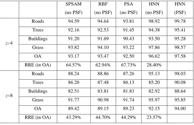
Table 4 SPM accuracy (%) of the different SPM schemes for the experiment on the land cover map 392
SPSAM
(no PSF)
RBF
(no PSF)
PSA
(no PSF)
HNN
(no PSF)
HNN
(PSF)
z=4
Roads 94.59 94.64 93.81 98.92 99.78
Trees 92.16 92.53 91.45 94.38 95.41
Buildings 91.20 91.69 90.43 93.50 95.28
Grass 93.82 94.10 93.22 97.86 98.57
OA 93.17 93.47 92.50 96.62 97.58
RRE (in OA) 64.57% 62.94% 67.73% 28.40%
z=8
Roads 88.24 88.86 87.26 95.13 98.03
Trees 86.20 87.48 86.13 85.20 90.08
Buildings 82.51 83.81 81.83 82.92 88.64
Grass 91.77 90.98 91.74 95.97 95.85
OA 89.42 89.15 89.23 92.15 94.00
RRE (in OA) 43.29% 44.70% 44.29% 23.57%
393
Table 4 is the accuracy for the five SPM methods, where two zoom factors, 4 and 8, were tested. Again, the
394
pure pixels were not considered in the accuracy statistics. For both zoom factors, the proposed HNN with PSF
395
method produces the greatest accuracy for all classes, and thus, the largest OA amongst all methods. More
396
specifically, SPSAM, RBF and PSA have very similar accuracies. The three methods produce OA of around 93%
397
for z=4 and 89% for z=8. Compared to the three benchmark methods, the HNN without PSF method is more
398
accurate. For z=4 and 8, the OA is increased by around 3.5% and 3%, respectively. With respect to the
399
proposed HNN with PSF method, the accuracies of roads, trees, buildings and grass are increased by at least
5%, 3%, 3.5% and 4% in comparison with SPSAM, RBF and PSA for z=4, and correspondingly, the OA is
401
increased by over 4%. In addition, with the PSF, the OA is 1% larger than the original HNN method. For z=8,
402
the accuracies of roads, trees and buildings for the proposed method are 3%, 5% and 6% larger than for the
403
HNN without PSF method. Moreover, the OA of the proposed method is 4.6%, 4.9%, 4.8% and 1.9% larger
404
than the SPSAM, RBF, PSA and HNN without PSF methods, and the corresponding RREs are 43.29%,
405
44.70%, 44.29% and 23.57%.
406
407
3.3. Experiment on the multispectral image
408
In this experiment, to control the experimental analysis and ensure the perfect reliability of the reference, a
409
synthesized multispectral image was used. The original multispectral image was acquired by the Landsat-7
410
Enhanced Thematic Mapper sensor in August 2001 and covers a farmland in the Liaoning Province, China.
411
The spatial resolution is 30 m. The studied area has a spatial size of 240 by 240 pixels and covers mainly four
412
land cover classes (marked as C1-C4). Fig. 8(a) and Fig. 8(b) show the original multispectral image and the
413
corresponding manually digitized reference map. From the reference map, the mean and variance of each land
414
cover class in the original 30 m Landsat image (bands 1-5 and 7 were considered) were calculated. Referring to
415
Fig. 8(b), the six-band 30 m resolution multispectral image was synthesized based on the random normal
416
distribution and the mean and variance of the classes. Fig. 8(c) shows the synthesized multispectral image. A
417
240 m coarse image, a spatial resolution comparable to that of medium-spatial-resolution systems such as
418
Moderate Resolution Imaging Spectroradiometer (MODIS), was created by degrading the synthesized 30 m
419
image with a factor of 8, using a Gaussian PSF. Fig. 8(d) shows the 240 m image. With this strategy, the
420
reference land cover map at 30 m is known perfectly for accuracy assessment.
421
Spectral unmixing was first performed on the 240 m coarse image using the classical linear spectral mixture
422
model. Fig. 9 is the relation between the estimated proportions and actual proportions for the four classes. The
423
errors are visually larger than those in Fig. 6. This is because the errors in proportions in this experiment
424
originate not only from the PSF effect, but also from the spectral unmixing process. This can be supported by
the results in Table 5, where the accuracies of the proportions were evaluated using two different references.
426
The convolved proportions were produced by convolving the 30 m land cover map in Fig. 8(b) with the
427
Gaussian PSF. Using the convolved proportions as reference, errors can be observed from only spectral
428
unmixing. As shown in the table, the spectral unmixing errors are particularly large for C1 and C2 (with
429
RMSEs of 0.0418 and 0.0303, respectively). Furthermore, as the PSF introduces additional uncertainty, the
430
accuracies evaluated using the actual proportions as reference are smaller than those for the convolved
431
proportions.
432
433
(a) (b) (c) (d) 434
[image:21.612.72.539.266.394.2]435
Fig. 8 The multispectral image used for experiment 3. (a) Original 30 m multispectral image (bands 432 as RGB). (b) Reference map 436
drawn manually from (a). (c) Synthesized 30 m multispectral image (bands 432 as RGB). (d) 240 m coarse image produced by 437
degrading (c) with a factor of 8 using a Gaussian PSF. 438
439
[image:21.612.98.518.499.603.2]440
Fig. 9 Relation between the actual proportions and proportions estimated from spectral unmixing for the multispectral image (z=8). 441
From left to right are results for C1-C4. 442
443
Based on the estimated proportions, SPM was implemented and the results of the five methods are shown in
444
Fig. 10. Failing to account for the PSF, the SPSAM, RBF and PSA predictions are dominated by noisy pixels
445
0 0.5 1
0 0.5 1 Actual proportions E st im a te d p ro p o rt io n s
0 0.5 1
0 0.5 1 Actual proportions E st im a te d p ro p o rt io n s
0 0.5 1
0 0.5 1 Actual proportions E st im a te d p ro p o rt io n s
0 0.5 1
and spurs on boundaries between classes. As the original HNN method is not completely slavish to the coarse
446
proportions, it can remove the noisy pixels and spurs and produce a smoother result than the SPSAM, RBF and
447
PSA. In Fig. 10(d), however, there are jagged boundaries, such as for C3 and C4. The prediction is further
448
enhanced by considering the PSF effect in the proposed method. The quantitative assessment in Table 6
449
suggests that the proposed method produces a larger accuracy for all four classes as well as a larger OA than the
450
other four SPM methods. Note that in this experiment, all pixels were considered in accuracy statistics,
451
including pure pixels. This is because whether a pixel is pure or not is determined by spectral unmixing and we
452
are concerned about the performance of spectral unmixing. The OA of the proposed method is 91.86%, with a
453
gain of more than 5% over SPSAM, RBF and PSA. Compared with the HNN without PSF, the proposed
454
method increases the accuracies of C1 and C4 by 4.5% and 5.5% and the OA by 1.3%. All RREs (in OA) are
455
large, which means that the proposed method reduces the errors obviously. Note that due to the uncertainty in
456
spectral unmixing, the OA of the proposed method is smaller than that for the land cover map in Table 2 (z=8).
457
[image:22.612.46.565.420.724.2]458
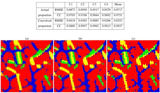
Table 5 Accuracy of the coarse proportion images for the multispectral image 459
C1 C2 C3 C4 Mean
Actual
proportion
RMSE 0.0873 0.0950 0.0517 0.0529 0.0717
CC 0.9703 0.9766 0.9844 0.9692 0.9751
Convolved
proportion
RMSE 0.0418 0.0303 0.0085 0.0206 0.0253
CC 0.9885 0.9957 0.9992 0.9913 0.9937
460
(a) (b) (c) 461
(d) (e) (f) 464
[image:23.612.45.567.51.241.2]465 466
Fig. 10 SPM results of the multispectral image with 240 by 240 pixels (z=8). (a) SPSAM (no PSF). (b) RBF (no PSF). (c) PSA (no 467
PSF). (d) HNN (no PSF). (e) The proposed HNN with PSF. (f) Reference. 468
469
Table 6 SPM accuracy (%) of the different SPM schemes for the experiment on the multispectral image 470
SPSAM
(no PSF)
RBF
(no PSF)
PSA
(no PSF)
HNN
(no PSF)
HNN
(PSF)
C1 75.88 77.65 75.98 76.89 81.40
C2 90.92 91.71 90.92 96.57 96.26
C3 82.50 84.30 81.68 87.08 89.81
C4 71.18 73.38 72.95 77.75 83.15
OA 85.91 87.07 85.95 90.57 91.86
RRE (in OA) 42.23% 37.05% 42.06% 13.68%
471
472
4. Discussion 473
474
The PSF effect exists ubiquitously in remote sensing images and the pixel signal is contaminated by its
475
neighbors as a result. Existing SPM methods are generally performed based on the assumption of the ideal
476
square wave filter-based PSF and treat the signal of a coarse pixel as the mean of sub-pixel signals within it.
477
This assumption ignores the effect from neighbors and limits unnecessarily the accuracy of SPM predictions.
478
As shown in the experimental results, the SPSAM, RBF and PSA predictions contain noticeable errors where
479
the PSF is ignored. Note that the performances of the SPSAM, RBF and PSA methods are not as satisfactory as
[image:23.612.134.478.337.481.2]demonstrated in the literature where they were proposed (Makido et al., 2007; Mertens et al., 2006; Wang et al.,
481
2014a). The reason is that in the experimental design in the literature, the coarse images were simulated using
482
the ideal square PSF and, thus, the sub-pixel maps can be satisfactorily reproduced by ignoring the PSF effect.
483
The proposed SPM approach that considers the PSF effect is developed based on the iterative HNN method.
484
The computing time is the product of the average time consumed in each iteration and the number of required
485
iterations. When considering the PSF effect, more sub-pixels are involved in the convolution process (see Eq.
486
(20)) and more time is needed in each iteration. Moreover, the convergence rate is slower and a larger number
487
of iterations is required. Thus, the proposed method has larger computational cost than the original HNN
488
method without the PSF. In the experiments, the original HNN method is able to converge after 1000 iterations,
489
but the proposed method needs 3000 iterations instead. For SPM of the multispectral image, the running time
490
of the original HNN and the proposed method is 1 and 5 hours, respectively. Note that the computational cost
491
of a SPM method is positively related to the spatial size of the input coarse image, number of classes and zoom
492
factor.
493
This paper considers using HNN to cope with the PSF effect. The solution is identified as modifying the
494
proportion constraint term in the original HNN using a convolution process where contributions from
495
neighboring coarse pixels are accounted for. It would be worthwhile to develop other solutions based on
496
existing SPM methods, such as PSA and the STHSPM methods. For example, in the original PSA method,
497
pixel swapping is allowed only within a coarse pixel. To account for the PSF, the SPM method can be extended
498
by allowing sub-pixel swaps not only within a coarse pixel, but also between coarse pixels. The number of
499
allowable sub-pixel swap between coarse pixels would be a key issue that needs to be addressed. Moreover, it
500
would also be interesting to consider developing artificial intelligence-based methods (e.g., genetic algorithm
501
and PSO, etc.). In such methods, the solutions in the set (called population in genetic algorithm and swarm in
502
PSO) can be updated iteratively according to the fitness values (calculated according to the pre-defined
503
objective) by using related operators (such as crossover and mutation in genetic algorithm and position update
504
in PSO). An optimal solution is expected to be produced after a number of generations. A critical issue for this
type of approach would be the definition of the objective, where a constraint term is needed for taking the PSF
506
effect into consideration. Both the prediction accuracy and computational cost will be important indices to
507
identifying an effective method.
508
Each sensor has its own PSF size. Based on the assumption of a Gaussian filter, some studies were
509
conducted to estimate the PSF size of satellite sensor images. Radoux et al. (2016) estimated the PSF size of
510
Landsat 8 and Sentinel-2 images. It was found that the full-width at half-maximum (FWHM) for Landsat 8 red
511
band is 1.70 pixels (amounting to a width of 0.72 pixel) and ranges from 1.67 to 2.21 pixels (i.e., a width from
512
0.71 to 0.94 pixel) for Sentinel-2 bands. Campagnolo & Montano (2014) estimated the PSF size of MODIS
513
images at different view zenith angles. The size of the PSF is a critical factor affecting the performance of the
514
proposed method, as displayed in Fig. 4. As the size increases, more neighboring sub-pixels contaminate the
515
center coarse pixel, and the accuracy of the proposed method will decrease correspondingly. However, the
516
advantage of the proposed method over the traditional method (i.e., accuracy gain) is obvious across different
517
PSF sizes, especially for large ones. The encouraging performance will promote the application of the
518
proposed method for sensors with various PSF sizes.
519
The main objective of this paper was to find a generic solution to address the PSF effect in SPM and increase
520
the accuracy of SPM predictions. A Gaussian PSF was assumed for convenience in the experimental validation.
521
In reality, the PSF may not be the Gaussian filter, especially for sensors with a rotating/scanning mirror which
522
will ensure that the shape has a directional component. For example, the MODIS sensor PSF was claimed to be
523
triangular in the along-scan direction but rectangular in the along-track direction in Tan et al. (2006). As seen
524
from Eq. (20), however, the proposed method is suitable for any PSF. Thus, in real cases, if the PSF is known
525
or estimated reliably, it can be used readily in the proposed method. This paper provides a first guidance to
526
increase SPM accuracy by considering the PSF effect. It could also help to initiate research on PSF estimation
527
that would ultimately provide the information needed for the use of the proposed method. The PSF estimation
528
mainly includes determination of the specific form of the function and related parameters. This is part of our
529
ongoing research.
The spatial clustering functions G1 and G2 in the HNN make the proposed method more appropriate for
531
SPM in the H-resolution case, where the objects of interest are larger than the pixel size of the input coarse
532
image (Atkinson, 2009). In the L-resolution case where the objects of interest are smaller than the pixel size,
533
alternative prior spatial structure information-based models, such as the semivariogram-based model in Tatem
534
et al. (2002), are more suitable, and should be applied. It would also be worthy of developing models that can
535
adaptively cope with different spatial patterns. Ge et al. (2016) performed a pioneering study for this issue.
536
Although the proposed method can increase the SPM accuracy, uncertainty still exists. Based on Eq. (6), the
537
ideal SPM solution is identified as the one that when convolved with the PSF, predicts the coarse proportion.
538
There can be multiple solutions satisfying this condition, leading to the perfect coherence constraint. The
539
uncertainty related to this issue can be further reduced by using additional information, such as sub-pixel
540
shifted remote sensing images (Ling et al., 2010; Zhong et al., 2014), panchromatic images (Ardila et al., 2011;
541
Li et al., 2014; Nguyen et al., 2011), high resolution color images (Mahmood et al., 2013), digital elevation
542
models (Huang et al., 2014), time-series images (Wang et al., 2016), segmentation data (Aplin & Atkinson,
543
2001; Robin et al., 2008) or shape information (Ling et al., 2012). It would be an interesting challenge to design
544
the appropriate model to incorporate such additional information into the proposed method considering the
545
PSF effect for possible enhancement in future research.
546
547
548
5. Conclusion 549
550
This paper presents a HNN-based method to account for the PSF effect in SPM and increase the SPM
551
predictions. Based on the recognition of the PSF as a real effect, the coarse proportions are viewed as the
552
convolution of sub-pixels within the local window centered at the coarse pixel, rather than of only the
553
sub-pixels within the coarse pixel. In the proposed HNN-based method, the interim SPM realization is
554
convolved with the PSF and compared with coarse proportions for further updating. The final solution is
identified as the one that when convolved with the PSF, is the same as the input coarse proportion. The
556
proposed method is a generic method suitable for any PSF. The effectiveness of the proposed method was
557
validated using three groups of datasets.
558
559
560
Acknowledgment 561
562
This work was supported in part by the Research Grants Council of Hong Kong under Grant PolyU
563
15223015. The authors would also like to thank the handling editor and three anonymous reviewers for their
564
valuable comments which greatly improved the work.
565
566
References 567
568
Aplin, P., & Atkinson, P. M. (2001). Sub-pixel land cover mapping for per-field classification. International Journal of Remote
569
Sensing, 22, 2853–2858. 570
Ardila, J. P., Tolpekin, V. A., Bijker, W., Stein, A. (2011). Markov-random-field-based super-resolution mapping for identification 571
of urban trees in VHR images. ISPRS Journal of Photogrammetry and Remote Sensing, 66, 762–775. 572
Atkinson, P. M. (1997). Mapping sub-pixel boundaries from remotely sensed images. Innov. GIS 4, 166–180. 573
Atkinson, P. M. (2005). Sub-pixel target mapping from soft-classified, remotely sensed imagery. Photogrammetric Engineering and
574
Remote Sensing, 71, 839–846. 575
Atkinson, P. M. (2008). Super-resolution mapping using the two-point histogram and multi-source imagery. GeoENV VI:
576
Geostatistics for Environmental Applications, 307–321. 577
Atkinson, P. M. (2009). Issues of uncertainty in super-resolution mapping and their implications for the design of an 578
inter-comparison study. International Journal of Remote Sensing, 30, 5293–5308. 579
Bioucas-Dias, J. M., Plaza, A., Dobigeon, N., Parente, M., Du, Q., Gader, P., Chanussot, J. (2012). Hyperspectral unmixing overview: 580
Geometrical, statistical and sparse regression-based approaches. IEEE Journal of Selected Topics in Applied Earth Observations
581
Boucher, A., & Kyriakidis, P. C. (2006). Super-resolution land cover mapping with indicator geostatistics. Remote Sensing of
583
Environment, 104, 264–282. 584
Campagnolo, M. L., & Montano, E. L. (2014). Estimation of effective resolution for daily MODIS gridded surface reflectance 585
products. IEEE Transactions on Geoscience and Remote Sensing, 52, 5622–5632. 586
Chen, Y., Ge, Y., Heuvelink, G. B. M., Hu, J., Jiang, Y. (2015). Hybrid constraints of pure and mixed pixels for soft-then-hard 587
super-resolution mapping with multiple shifted images. IEEE Journal of Selected Topics in Applied Earth Observations and
588
Remote Sensing, 8, 2040–2052. 589
Foody G. M., & Doan, H. T. X. (2007). Variability in soft classification prediction and its implications for sub-pixel scale change 590
detection and super-resolution mapping. Photogrammetric Engineering and Remote Sensing, 73, 923-933. 591
Ge, Y., Chen, Y., Li, S., Jiang, Y. (2014). Vectorial boundary-based sub-pixel mapping method for remote-sensing imagery. 592
International Journal of Remote Sensing, 35, 1756–1768. 593
Ge, Y., Chen, Y., Stein, A., Li, S., Hu, J. (2016). Enhanced subpixel mapping with spatial distribution patterns of geographical 594
objects. IEEE Transactions on Geoscience and Remote Sensing, 54, 2356–2370. 595
Gu, Y., Zhang, Y., Zhang, J. (2008). Integration of spatial-spectral information for resolution enhancement in hyperspectral images. 596
IEEE Transactions on Geoscience and Remote Sensing, 46, 1347–1358. 597
Heinz, D. C., & Chang, C. I. (2001). Fully constrained least squares linear spectral mixture analysis method for material 598
quantification in hyperspectral imagery. IEEE Transactions on Geoscience and Remote Sensing, 39, 529–545. 599
Kasetkasem, T., Arora, M. K., Varshney, P. K. (2005). Super-resolution land-cover mapping using a Markov random field based 600
approach. Remote Sensing of Environment, 96, 302–314. 601
Keshava N., & Mustard, J. F. (2002). Spectral unmixing. IEEE Signal Processing Magazine, 19, 44–57. 602
Huang, C., Townshend, R.G., Liang, S., Kalluri, S. N. V., DeFries, R. S. (2002). Impact of sensor’s point spread function on land 603
cover characterization: assessment and deconvolution. Remote Sensing of Environment, 80, 203–212. 604
Huang, C., Chen, Y., Wu, J. (2014). DEM-based modification of pixel-swapping algorithm for enhancing floodplain inundation 605
mapping. International Journal of Remote Sensing, 35, 365–381. 606
Li, L., Chen, Y., Xu, T., Liu, R., Shi, K., Huang, C. (2015). Super-resolution mapping of wetland inundation from remote sensing 607
imagery based on integration of back-propagation neural network and genetic algorithm. Remote Sensing of Environment, 164, 608
142–154. 609
Li, X., Ling, F., Du, Y., Zhang, Y. (2014). Spatially adaptive superresolution land cover mapping with multispectral and 610