Slicing COSMOS with SC4K:the evolution of typical Lya emitters and the Lya escape fraction from z~2 to z~6

Slicing COSMOS with SC4K: the evolution of typical Ly

α

emitters and the Ly

α

escape fraction from z

_∼

2 to z

_∼

6

David Sobral

, S´ergio Santos

, Jorryt Matthee

, Ana Paulino-Afonso

,

Bruno Ribeiro

, Jo˜ao Calhau

, Ali A. Khostovan

1 _{Department of Physics, Lancaster University, Lancaster, LA1 4YB, UK}

2 _{Leiden Observatory, Leiden University, P.O. Box 9513, NL-2300 RA Leiden, The Netherlands}

3 _{Instituto de Astrof´ısica e Ciˆencias do Espa¸co, Universidade de Lisboa, OAL, Tapada da Ajuda, PT1349-018 Lisboa, Portugal} 4 _{Departamento de F´ısica, Faculdade de Ciˆencias, Universidade de Lisboa, Edif´ıcio C8, Campo Grande, PT1749-016 Lisboa, Portugal} 5 _{Centro de Computa¸c˜ao Gr´afica, CVIG, Campus de Azur´em, PT4800-058 Guimar˜aes, Portugal}

6 _{Department of Physics and Astronomy, University of California, 900 University Ave., Riverside, CA 92521, USA}

Accepted 2018 February 9. Received 2018 February 7; in original form 2017 December 12

ABSTRACT

We present and explore deep narrow- and medium-band data obtained with the Subaru and the Isaac Newton telescopes in the ∼2 deg2 _{COSMOS field. We use these data} as an extremely wide, low-resolution (R_∼20₋80) IFU survey to slice through the COSMOS field and obtain a large sample of ∼4000 Lyαemitters (LAEs) fromz∼2 toz_∼6 in 16 redshift slices (SC4K). We present new Lyαluminosity functions (LFs) covering a co-moving volume of _∼ 108_Mpc3_{. SC4K extensively complements} ultra-deep surveys, jointly covering over 4 dex in Lyα luminosity and revealing a global (2.5< z <6) synergy LF with α=₋1.93₋+0₀._.12₁₂, log10Φ∗Lyα =−3.45

+0.22

−0.29Mpc−3 and log10L∗Lyα = 42.93

+0.15

−0.11erg s−1. The Schechter component of the Lyα LF reveals a factor _∼5 rise in L∗

Lyα and a ∼7× decline in ΦLy∗ α from z ∼2 to z ∼6. The data reveal an extra power-law (or Schechter) component above LLyα ≈ 1043.3erg s−1 at

z_∼2.2₋3.5 and we show that it is partially driven by X-ray and radio AGN, as their LyαLF resembles the excess. The power-law component vanishes and/or is below our detection limits abovez >3.5, likely linked with the evolution of the AGN population. The Lyαluminosity density rises by a factor∼2 fromz∼2 toz∼3 but is then found to be roughly constant (1.1+0₋0..22×1040erg s−1Mpc−3) toz∼6, despite the∼0.7 dex drop in UV luminosity density. The Lyα/UV luminosity density ratio rises from 4±1% to 30_±6% fromz _∼2.2 to z _∼6. Our results imply a rise of a factor of_≈2 in the global ionisation efficiency (ξion) and a factor_≈4_±1 in the Lyαescape fraction from

z∼2 toz∼6, hinting for evolution in both the typical burstiness/stellar populations and even more so in the typical ISM conditions allowing Lyαphotons to escape.

Key words: galaxies: evolution; galaxies: high-redshift; galaxies: luminosity function; cosmology: observations.

1 INTRODUCTION

Understanding how galaxies form and evolve across cosmic time is a complex challenge which requires identifying and studying the inter-dependencies of key physical mechanisms over a range of environments (see e.g. Schaye et al. 2015; Crain et al. 2015; Henriques et al. 2015; Muldrew et al. 2018), informed by a variety of observations (e.g. Muzzin et al. 2013). It is now well established that the star for-mation rate density (SFRD) of the Universe evolves with

? _{E-mail: [email protected]}

redshift, peaking atz_∼2₋3 (e.g.Lilly et al. 1996;Karim et al. 2011;Sobral et al. 2013;Madau & Dickinson 2014) and declining at even higher redshift (e.g.Bouwens et al. 2015; Khostovan et al. 2015), but several questions related to the physics of such evolution remain unanswered.

In order to unveil the evolution of physical properties of galaxies and active galactic nuclei (AGN) across time one requires self-consistent selection methods which can be ap-plied across redshift. The Lyman Break selection (e.g.Koo & Kron 1980;Steidel & Hamilton 1993;Giavalisco et al. 1996) has been successfully used to produce large samples of galax-ies up toz _∼10 (e.g.McLure et al. 2010;Ellis et al. 2013;

Bouwens et al. 2014a,b;Finkelstein 2016;Bielby et al. 2016) through extremely deep optical to near-infrared (NIR) ob-servations. However, UV-continuum selected samples using the Hubble Space Telescope (HST) are typically too faint (e.g. Atek et al. 2015) for extensive spectroscopic follow-up, particularly when probing distant look-back times (but large area surveys can still provide ideal follow-up targets e.g. Bowler et al. 2014,2017). One alternative is to select galaxies by their Hydrogen nebular recombination lines, such as Hαin the rest-frame optical (e.g.Sobral et al. 2013; Col-bert et al. 2013) or Lyman-α(Lyα;λ0 = 1215.67 ˚A) in the

rest-frame UV.

Lyα is intrinsically the strongest emission line in the rest-frame optical and UV (e.g. Partridge & Peebles 1967; Pritchet 1994) and it is routinely used to select high redshift sources (z_∼2₋7; see e.g.Malhotra & Rhoads 2004). Lyαis expected to be emitted by young star-forming galaxies (e.g. Charlot & Fall 1993;Pritchet 1994), but it is also observed around AGN (e.g. Miley & De Breuck 2008). Searches for Lyαemitters (LAEs) have created samples of thousands of galaxies/AGN, including sources that are too faint to be de-tected by continuum based searches (e.g.Bacon et al. 2015). The techniques used to detect LAEs include narrow-band surveys (e.g. Rhoads et al. 2000;Westra et al. 2006;Ouchi et al. 2008;Hu et al. 2010;Matthee et al. 2015;Konno et al. 2017;Zheng et al. 2017), Integral Field Unit (IFU) surveys (e.g.van Breukelen et al. 2005;Bacon et al. 2015;Drake et al. 2017a) and blind slit spectroscopy (e.g. Martin & Sawicki 2004;Rauch et al. 2008;Cassata et al. 2011,2015). Galax-ies selected through their Lyαemission allow for easy spec-troscopic follow-up due to their high EWs (e.g.Hashimoto et al. 2017) and typically probe low stellar masses (see e.g. Gawiser et al. 2007;Hagen et al. 2016;Oyarz´un et al. 2017). Narrow-band and/or IFU surveys have the added benefit of being truly blind, and thus allow a good assessment of the volume and selection completeness.

Unfortunately, inferring intrinsic properties of galaxies from Lyαobservations alone can be challenging due to the highly complex resonant nature of this emission line (for a review on the physics of Lyαradiative transfer see e.g. Dijk-stra 2017). A significant fraction of Lyαphotons is scattered by the Inter-Stellar Medium (ISM), increasing the likeli-hood of being absorbed by dust, and in the Circum-Galactic Medium (CGM) as evidenced by the presence of extended Lyαhalos (e.g. Momose et al. 2014; Wisotzki et al. 2016). Therefore, the Lyαescape fraction1(fesc; see e.g.Atek et al.

2008), the ratio between the observed and the intrinsically produced Lyαluminosity from a galaxy, is still poorly un-derstood quantitatively. New studies are now directly mea-suring fesc of large samples of galaxies and over a range of

redshifts by obtaining Hαand Lyαobservations simultane-ously (seeNakajima et al. 2012;Matthee et al. 2016;Sobral et al. 2017b;Harikane et al. 2017). For example, fescis found

to be anti-correlated with stellar mass (e.g. Matthee et al. 2016;Oyarz´un et al. 2017), dust attenuation (e.g.Verhamme et al. 2008;Hayes et al. 2011;Matthee et al. 2016) and SFR (e.g.Matthee et al. 2016). Interestingly, the LyαEW0seems

to be the simplest empirical predictor of fescin LAEs with a

1 _{Throughout this study we use fescto quantify the escape}

frac-tion of Lyαphotons, not Lyman-continuum photons.

relation that shows no evolution fromz∼0 toz∼2 (Sobral et al. 2017b) and that may remain the same all the way to

z∼5 (Harikane et al. 2017).

“Typical” star-forming galaxies at z ∼ 2 have low fesc

(_∼1₋5%; e.g.Oteo et al. 2015;Cassata et al. 2015), likely because the dust present in their ISM easily absorbs Lyα

photons (e.g.Ciardullo et al. 2014;Oteo et al. 2015;Oyarz´un et al. 2017) and prevents most Lyαemission from escaping (see e.g.Song et al. 2014). However, sources selected through their Lyαemission typically have _∼10 times higher escape fractions (e.g.Song et al. 2014;Sobral et al. 2017b), with Lyαescaping over _≈2_× larger radii than Hα(e.g. Sobral et al. 2017b). Furthermore, due to the sensitivity of fesc to

neutral Hydrogen, Lyαcan be used as a proxy of the ISM neutral gas (HI) content (Trainor et al. 2015;Konno et al. 2016) and the dust content (Hayes et al. 2011).

Statistically, the number density of LAEs as a function of luminosity (the luminosity function, LF), encodes valu-able information on the global properties of LAEs and Lyα

emission. Observations have revealed that the Lyα LF re-mains roughly constant atz_∼3₋6 (e.g.Ouchi et al. 2008; Santos et al. 2016; Drake et al. 2017a). This is in princi-ple unexpected, as the cosmic SFRD, as traced by the UV LF, drops significantly at those redshifts (e.g.Bouwens et al. 2015;Finkelstein et al. 2015) and implies that intrinsic prop-erties of galaxies may be evolving, on average, with redshift. Those may include lower dust content, leading to a higher fescwhich could compensate for a lower intrinsic production

of Lyαphotons (e.g.Hayes et al. 2011;Konno et al. 2016). Another possibility is that ξion, which measures the ratio

between ionising (LyC) and UV flux density increases with redshift (e.g. Duncan & Conselice 2015; Khostovan et al. 2016; Matthee et al. 2017a). In practice, a combined in-crease of bothξionand fesc is also possible, which could tell

us about an evolution of both the typical stellar popula-tions/burstiness but also on the evolving physics/ISM con-ditions) of the escape of Lyαphotons.

In this work, we use 16 different narrow- and medium-band filters over the COSMOS field to select a large sample of LAEs in a total co-moving volume of 6.4_×107_Mpc3 _and

a wide redshift range ofz _∼2₋6, addressing the current shortcomings of deep, small area surveys. Our survey can be seen as a very wide (_≈2 deg2_{), low resolution IFU}

sur-vey between 400-850 nm, probing LAEs from the end of the epoch of re-ionisation atz_∼6 (e.g.Fan et al. 2006) to the peak of star-formation history atz∼2−3.

We structure this paper as follows: Section2presents the data and the extraction of sources. Section 3presents the selection of line emitters, the criteria we applied to select LAE candidates atz_∼2₋6 and the final SC4K sample. We present the methods in Section4, including all the steps and corrections in determining LyαLFs. Results are presented in Section 5, including the evolution of the Lyα LF with redshift, comparisons with other surveys, the synergy LF (S-SC4K) and the evolution of the Lyαluminosity density. We discuss our results in Section6, including how fesc and

ξion likely evolve with redshift. Finally, Section 7presents

the conclusions of this paper. Throughout this work we use a ΛCDM cosmology with H0= 70 km s−1Mpc−1, ΩM = 0.3 and ΩΛ= 0.7. All magnitudes in this paper are presented in

0.2

0.4

0.6

0.8

1.0

u B g V r+

i+

z+

NB392 NB501 NB711 NB816

3000

4000

5000

6000

7000

8000

9000

10000

0.2

0.4

0.6

0.8

1.0

IA464 IA484 IA505 IA527 IA574 IA624 IA679 IA709 IA738 IA767 IA827

2.0

3.0

Redshifted Ly

4.0

5.0

↵

6.0

7.0

Observed wavelength ( ˚A)

N

or

m

al

ise

d

Tr

an

sm

issi

on

Figure 1.Normalised filter profiles used in this paper. The top axis indicates the redshift of Lyαemission for the corresponding observed wavelength.Top:The broad-bands (u,B,g,V,r+_,i+_andz+_{; typical FWHM∼100 nm) which we use to estimate the continuum for}

candidate line-emitters and four narrow-bands which we also present in our final catalogue (NB392, NB501, NB711 and NB816; typical FWHM∼10 nm).Bottom:The 12 medium-bands used in this study (typical FWHM∼30 nm; see Table1) which are sensitive to Lyα

emission fromz∼2.5 toz∼5.8. Note that some of the medium-band filters overlap slightly, which can result in some sources being detected as LAEs in two consecutive medium bands, although we note that the overlapping volume is always relatively small.

2 DATA AND SOURCE EXTRACTION

The COSMOS field (Scoville et al. 2007;Capak et al. 2007) is one of the most widely studied regions of extragalactic sky, with a plethora of publicly available multi-wavelength cov-erage. Data in COSMOS include X-ray, UV, optical, NIR, FIR and radio (see e.g. Ilbert et al. 2009; Civano et al. 2016; Laigle et al. 2016; Smolˇci´c et al. 2017). We explore a range of narrow- and medium-band data (Capak et al. 2007;Taniguchi et al. 2007,2015a;Santos et al. 2016; So-bral et al. 2017b;Matthee et al. 2017b) over roughly the full COSMOS field in order to 1) create detection-catalogues for each band, 2) identify sources with strong excess emission in those bands relative to their broad-band counterparts and 3) obtain dual-mode photometry on all other bands avail-able in order to further constrain the (photometric-)redshift of each source. In Figure1we show the filter profiles of all the 12 medium-bands and the 4 narrow-bands used in this paper. These filters are capable of detecting various emission lines, particularly redshifted Lyα spanning a wide redshift range, fromz_∼2 toz_∼6.

2.1 Medium-band data

We retrieve the publicly available medium-band data (see Table1and Figure1) from the COSMOS archive (seeIlbert et al. 2009;Taniguchi et al. 2015a). All data were obtained with the Suprime-Cam (S-Cam) instrument on the Subaru

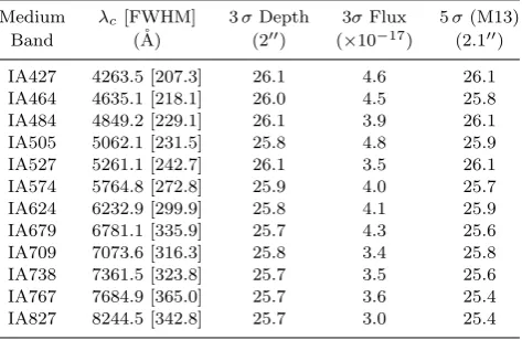
Table 1.The medium-band filters (seeTaniguchi et al. 2015a) and the depth of the data obtained with them, measured directly (3σ; 5σ can be obtained by subtracting 0.5) in 200 apertures and byMuzzin et al. 2013 (M13). We also transform our mea-sured 3σ limiting magnitude (200_{) into a flux limit (in units of} erg s−1_cm−2_{) in the case of the full flux within the 2}00 medium-band aperture being from an emission line.

Medium λc[FWHM] 3σDepth 3σFlux 5σ(M13)

Band (˚A) (200_{) (}×10−17_{) (2.1}00₎

IA427 4263.5 [207.3] 26.1 4.6 26.1

IA464 4635.1 [218.1] 26.0 4.5 25.8

IA484 4849.2 [229.1] 26.1 3.9 26.1

IA505 5062.1 [231.5] 25.8 4.8 25.9

IA527 5261.1 [242.7] 26.1 3.5 26.1

IA574 5764.8 [272.8] 25.9 4.0 25.7

IA624 6232.9 [299.9] 25.8 4.1 25.9

IA679 6781.1 [335.9] 25.7 4.3 25.6

IA709 7073.6 [316.3] 25.8 3.4 25.8

IA738 7361.5 [323.8] 25.7 3.5 25.6

IA767 7684.9 [365.0] 25.7 3.6 25.4

IA827 8244.5 [342.8] 25.7 3.0 25.4

depth (Muzzin et al. 2013) but with some exceptions (see Table1), varying from 26.2 mag (deepest: IA427, IA484 and IA527) to 25.4 mag (shallowest, IA767), measured in 2.100 apertures (5σ, seeMuzzin et al. 2013). We also obtain our own depth measurements by placing 100,000 empty/random 200apertures in each of the (native) images and determining the standard deviation. The results are presented in Table 1and compared with the depths measured inMuzzin et al. (2013), who used PSF-matched data.

2.2 Narrow-band data

We complement our medium-band data with four narrow-band studies in the COSMOS field: the CALYMHA sur-vey at z = 2.2 (Sobral et al. 2017b) and az = 3.1 survey (Matthee et al. 2017b) using the narrow-band filters NB392 and NB501, respectively, both mounted on the 2.5 m Isaac Newton Telescope’s WFC. The NB392 data (λc= 392 nm, ∆λ= 5.2 nm;Sobral et al. 2017b) have a 5σdepth of 23.7-24.5 AB magnitude and a typical PSF-FWHM of 1.800. The NB501 data (λc= 501 nm, ∆λ= 10 nm) were taken and re-duced with a similar strategy and data-quality as the NB501 data described inMatthee et al.(2017b) and have a typical 5σdepth of 24.0 AB magnitude with 1.600PSF-FWHM. Lim-iting magnitudes for NB392 and NB501 data were measured with 300_apertures.

In addition, we also use two narrow-band surveys ex-ploring S-Cam data: z = 4.8 (Perez et al. in prep) and

z = 5.7 (Santos et al. 2016); these have used the narrow-band filters NB711 and NB816, respectively (see Figure1). We note that all NB and MB selected catalogues have been obtained in similar ways, which we describe in Section2.3.

2.3 Extraction of sources

To produce the narrow- or medium-band selected catalogues (see e.g.Matthee et al. 2017b), we followSantos et al.(2016). Briefly, we start by registering theu, B,g,V,r+, i+,z+,

Y, J, H andK (Taniguchi et al. 2007;Capak et al. 2007; McCracken et al. 2012) and all the medium-band (or narrow-band) images to a common astrometric reference frame using

Swarp(Bertin et al. 2002). We extract sources with a

pri-mary 200aperture2 (but we note we also extract them with multiple apertures, includingmag-auto, a proxy of the total magnitude) usingSExtractor(Bertin & Arnouts 1996) in dual-image mode, and with each of the medium-band images as the detection image. Therefore, for each medium-band, we create a catalogue with all the detections on that band, and with the broad-band photometry extracted at the coordi-nates of each detection. We thus note that our selection is purely based on the detection of a source in a medium- or narrow-band, independently of its continuum strength.

Before creating our final catalogues, we investigate the need for any significant masking to remove low quality re-gions and diffraction patterns around bright stars. In addi-tion to removing such regions, we also find that there is a small area in the corner of the COSMOS field (_≈0.02 deg2₎

for which there is no u-band data. Given that we require

2 _{Because the NB392 and NB501 data have a broader PSF,}

pho-tometry has been done with 300apertures.

Table 2.The estimated depth of broad-band data used in our analysis (3σ). We measure these by placing 100,000 random 200 empty apertures, and computing the standard deviation of the counts and converting it to magnitudes. The 2σ and 4σ limits can be obtained by adding 0.44 and subtracting 0.31, respectively.

u3σ B3σ V3σ g3σ r3+σ i+3σ z3+σ

26.81 27.21 26.50 26.61 26.55 26.12 25.23

blue photometry to select LAEs and reject lower redshift sources (see Tables 2and 3), we mask/exclude this region for filters bluer than IA574. After masking, the contiguous survey area is 1.94-1.96 deg2_{for the medium-band filters and}

1.96 deg2 for the NB711 and NB816 filters, while the area covered by the NB392 and NB501 data is 1.21 deg2 _{and 0.85}

deg2, respectively (Matthee et al. 2016;Sobral et al. 2017b).

3 SELECTION CRITERIA: SC4K

3.1 Selection of candidate line-emitters

In order to identify sources with candidate emission lines out of all medium-band selected sources, it is necessary to estimate the continuum of each source. As the central wave-lengths of medium-bands are typically offset (see Figure1) from the central wavelengths of their overlapping broad-band, we need to investigate and apply a correction to the medium band photometry (MB0). This step/correction

as-sures that a measured medium-band excess is not dependent on the intrinsic slope of the continuum (estimated with two broad-band magnitudes, BB₋BBadjacent), similarly to

cor-rections applied for narrow-band surveys (e.g.Sobral et al. 2013; Vilella-Rojo et al. 2015). Without such correction, sources with significant colours could mimic emission lines. In practice this requires re-calibrating either MB0 or BB

photometry (or producing a new artificial BB magnitude) to assure that, on average, sources without an emission-line will have a zero colour excess (BB₋MB_≈0) regardless of their continuum colour (BB−BBadjacent). We do this by

evaluat-ing the colour dependence of BB₋MB0 on BB−BBadjacent

and parameterising it as (calculatingmandb):

BB₋MB0=m×(BB−BBadjacent) +b (1)

We then use coefficientsmandbto finally obtain:

MB = MB0+ (m×(BB−BBadjacent) +b) (2)

with the filters listed in Table 3. The coefficients m and

b are provided in Table A2. We note that for some filter combinations bothmandbare effectively zero. For sources without BB₋BBadjacent(<2σdetection in either band) we

compute a median correction which we apply per medium-band filter. Typical median corrections are at the 0.1 mag level and in the 0.0-0.3 range (see TableA2).

20 21 22 23 24 25

IA427 (AB, 2”)

-1 0 1 2 B -I A 42 7

EW0>50˚A

⌃>3(average)

20 21 22 23 24 25

IA464 (AB, 2”)

-1 0 1 2 B -I A 46 4

20 21 22 23 24 25

IA484 (AB, 2”)

-1 0 1 2 B -I A 48 4

20 21 22 23 24 25

IA505 (AB, 2”)

-1 0 1 2 V -I A 50 5

EW0>50˚A

⌃>3(average)

20 21 22 23 24 25

IA527 (AB, 2”)

-1 0 1 2 V -I A 52 7

20 21 22 23 24 25

IA574 (AB, 2”)

-1 0 1 2 r +-I A 57 4

20 21 22 23 24 25

IA624 (AB, 2”)

-1 0 1 2 r +-I A 62 4

EW0>50˚A

⌃>3(average)

20 21 22 23 24 25

IA679 (AB, 2”)

-1 0 1 2 r +-I A 67 9

20 21 22 23 24 25

IA709 (AB, 2”)

-1 0 1 2 i +-I A 70 9

20 21 22 23 24 25

IA738 (AB, 2”)

-1 0 1 2 i +-I A 73 8

EW0>50˚A

⌃>3(average)

All MB detections All candidate line-emitters Candidate LAEs after visual checks

20 21 22 23 24 25

IA767 (AB, 2”)

-1 0 1 2 i +-I A 76 7

20 21 22 23 24 25

IA827 (AB, 2”)

-1 0 1 2 i +-I A 82 7

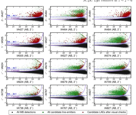
Figure 2.The colour-magnitude diagrams used for the selection of line-emitters for the 12 medium-bands. Each medium-band magnitude is plotted versus the excess colour, and we identify sources with a high enough EW (corresponding to a rest-frame EW of>50 ˚A for LAEs) and with a significant excess (average Σ>3). The selection criteria of LAEs are presented in Table3. MB detections are shown in black, candidate line-emitters (prior to individual visual checks) are shown in green and candidate LAEs in red (after visually checking all of them). We assign the broad-band detection limit to sources with no broad-band detection. It is clear from the panels that, on average, the amount and fraction of LAEs greatly decreases from the bluer (where almost all candidate line-emitters are LAEs) to the redder filters (where only a small fraction is consistent with being a LAE).

noise a given colour excess (due to a potential emission line) is and can be written as (Sobral et al. 2013):

Σ = 1−10−

0.4(BB−MB)

10−0.4(ZP₋MB)p rms2

BB+ rms2MB

, (3)

where BB and MB are the broad- and the medium-band magnitudes andZP is the zero-point of the image. We esti-mate rmsMB and rmsBB by randomly placing 200apertures

in the appropriate images and determining the standard de-viation per image. This approach takes spatially correlated noise into account. We apply an emission-line significance threshold of Σ>3, similarly to other studies (e.g.Matthee et al. 2015). In addition to Σ, we also measure the observed EW (EWobs) of potential lines as:

EWobs= ∆λMB

fMB−fBB

fBB−fMB(∆λMB/∆λBB)

, (4)

where ∆λMB and ∆λBB are the FWHM of the

medium-(see Table 1) and broad-band filters (Capak et al. 2007;

Taniguchi et al. 2015a), and fMB and fBBare the flux

densi-ties3 _{measured of the two filters.}

Typical narrow-band surveys apply a Lyα rest-frame EW (EW0) cut of≈25 ˚A (e.g.Ouchi et al. 2008), mostly to

avoid contamination from other line-emitters, as Lyαis typ-ically the line with the highest observed EW (but see also other high EW contaminants in e.g.Sobral et al. 2017b). Re-cent surveys also explored lowering this cut, showing that a few extra real Lyαsources may be recovered in those cases, which can populate the bright end (Sobral et al. 2017b, see also VUDS, e.g.Le F`evre et al. 2015), but also introduce many extra contaminants. Given that we are using wider fil-ters in comparison to the typical narrow-band filfil-ters, we are forced to use a higher observed EW cut to retrieve clean

sam-3 _{Note that as a consequence of the way we define/correct MB}

magnitudes, their flux densities (Fλ) need to be calculated with

1000 1500 2000 2500 3000 3500 4000 4500 5000 5500 6000 6500

Central rest-frame wavelength probed by MB filter ( ˚A, from photometric or spectroscopic redshift)

0 200 400 600 800 1000 1200

N

um

be

ro

fso

ur

ce

s

Ly

↵

[O

]

H

[O

]

H

↵

Candidate line-emitters Candidate LAEs

Sources with public zspec⇥10

Figure 3. Distribution of the central rest-frame wavelengths probed by the different medium-band filters (based on photometric or spectroscopic redshifts) of our continuum-bright (with accurate photometric redshifts) sample of line-emitters (green histogram) and its subset containing only our final LAEs (red histogram). The photometric redshifts used in this figure are taken fromLaigle et al.(2016). We convert each photometric value to a rest-frame wavelength assuming the source has an emission line at the central wavelength of the corresponding medium-band. The black dashed lines are the rest-frame wavelengths of the main emission lines probed. Our sample of continuum-bright line-emitters is clearly dominated by Lyαemitters, followed by a population of Hαemitters, [Oiii]+Hβemitters, and finally [Oii] emitters. We find that our Lyαselection criteria is able to remove the vast majority of lower redshift contaminants whilst maintaining the bulk of Lyαphotometric candidates (see Section3.3).

ples of line-emitters. For our analysis, we find that setting an observed EW cut from 175 ˚A to 340 ˚A from the bluest (nar-rowest) to the reddest and broader filters is able to recover clean samples of line emitters and yields an homogeneous rest-frame Lyαequivalent width cut of EW0 >50 ˚A for all

of our medium-bands. Note that our EW0 cut (for LAEs) is

about twice the typical used in narrow-band surveys (25 ˚A; see e.g.Santos et al. 2016), implying we are likely less con-taminated by lower redshift line-emitters, but that we may be less complete. We take this into account when deriving completeness corrections, but we note that, in practice, the vast majority of LAEs at high redshift show EW0 >50 ˚A;

see e.g.Ouchi et al.(2008). For an in-depth analysis of select-ing LAEs with different EW0 cuts seeSobral et al.(2017b)

and Perez et al. (in prep.).

The full selection procedure to search for candidate emission-line sources is illustrated in Figure2, which shows the medium-band colour excess versus medium-band mag-nitude for each band. It can be seen that the EW threshold is well above the scatter at bright magnitudes (. 23). In total, we identify 40,726 potential line-emitters, with each medium-band contributing with roughly 2,000-3,000 emit-ters to the sample. We note, nonetheless, that we expect our full sample of _≈40 k candidate line-emitters to still be contaminated by e.g. artefacts around bright stars, cosmic rays, and due to other image defects. In order to fully ad-dress this possibility, we visually inspect every single source in our final sample (see Section3.4), but we first filter out lower redshift emitters and isolate candidate LAEs.

3.2 Photometric and spectroscopic redshifts

In order to test how robust our emission-line selection crite-ria are, we use a large compilation of photometric and spec-troscopic redshifts (e.g. Lilly et al. 2007;Ilbert et al. 2009; Laigle et al. 2016). We use the distribution of photometric redshifts to identify the likely rough rest-frame wavelength of each emission-line picked up by the medium-bands, and show the results in Figure3. We find evidence for the

pres-ence of a large population of Hβ+[Oiii]5007and Hαemitters,

although the sample is dominated by candidate LAEs. Ex-cluding the dominating LAEs, the most common remaining sources are Hα emitters, followed by [Oiii]+Hβ. [Oii]3727

emitters represent a less frequent population among all the candidate line-emitters, and we also find evidence for some 4000 ˚A and Lyman break sources making it to the sample of potential line emitters. The relative proportion of sources is not surprising, given the combination of volume and ob-served EW distributions of all these lines (see e.g. Sobral et al. 2014;Khostovan et al. 2016;Hayashi et al. 2017).

While Figure3shows that our sample of high EW can-didate line-emitters is dominated by LAE cancan-didates, it also reveals that many other line-emitters are expected to be in the sample. This is confirmed by spectroscopic redshifts of the full sample and stresses the importance of excluding lower redshift emitters in order to produce relatively clean and complete samples of LAEs.

3.3 Selection of LAEs at z_∼2.5₋6

In order to isolate LAEs from lower redshift line-emitters (see Figure3), we apply two criteria. First, we identify the presence of a colour break blue-ward of the medium-band ex-cess emission and no significant emission bluer of that (see Table2). Secondly, we remove sources that have red colours (e.g.B₋r >0.5 forz_∼2.5;i₋z >1.0 forz_∼5.5); see Table 3. The first step selects the Lyman break, while the second criterion removes sources likely to be stars or red galax-ies with a strong Balmer break (at a rest-frame wavelength ∼400 nm) that mimics the Lyman break (see e.g.Matthee et al. 2014, 2017c). Narrow-band surveys for LAEs typi-cally apply the same/similar standard criteria (e.g. Ouchi et al. 2008;Matthee et al. 2015;Bielby et al. 2016;Santos et al. 2016), with the difference being how strict the cri-teria/flexible the cuts are and what bands are available to trace/identify the Lyman break. Some surveys conducted in the blue bands rely mostly on a high EW0 cut (e.g.

Table 3. The selection of LAEs from the sample of all line-emitters, using an observed EW threshold of EW >50×(1 +z) ˚A and Σ > 3. The relevant LAE colour selection is given in the table. Numbers of LAEs are given after visually inspecting all candidate LAEs and rejecting interlopers. As described in the Section3.3, colour criteria are based on the Lyman break technique and removing sources with very red colours red-wards of the emission-line (which indicates that the potential Lyman break is actually a Balmer break and that the line is not Lyα). We note that we explicitly perturb these colour selections with Markov chain Monte Carlo (MCMC) simulations and include the results in the errors when we estimate luminosity functions. We remove 20 confirmed lower redshift line emitters/contaminants, as described in Section3.5and we expect a≈10−20% remaining contamination. Due to a small overlap of some of the medium filters in their wings a small number (53;∼1%) of LAEs are detected as LAEs in two adjacent MB filters; these are kept in each of the filters for the full analysis.1_EW

0>5 ˚A;Sobral et al.(2017b)2EW0>25 ˚A;Santos et al.(2016);Matthee et al.

(2017b); Perez et al. in prep.

Selection Excess Lyαredshift LAE colour selection # LAE

filter filter FWHM (Section3.3) candidates

IA427 B(u) 2.42−2.59 (u > u3σ∨u−B >0.4) & (B−r+<0.5) 741

IA464 B(V) 2.72−2.90 (u > u3σ∨u−B >0.5) & (B−r+<0.8) 311

IA484 B(V) 2.89−3.08 (u > u3σ ∨u−B >0.5) & (B−r+<0.75) 711

IA505 V (B) 3.07−3.26 (u > u3σ∨u−V >1.3) & (B−r+<0.5) 483

IA527 V (B) 3.23−3.43 (u > u3σ ∨u−V >1.5) & (V −i+<1.0) 641

IA574 r+_{(V) 3.63−3.85 (u > u}

3σ) & (B > B3σ ∨B−r+>1.0) & (V −i+<0.5) 98

IA624 r+_(i+_{) 4.00−4.25 (B > B}

3σ) & (V > V3σ ∨V −r+>0.5) & (r+−i+<1.0) 142

IA679 r+_(i+_{) 4.44−4.72 (B > B}

3σ) & (V > V3σ ∨V −r+>0.5) & (r+−i+<1.0) 79

IA709 i+ _(r+_{) 4.69−4.95 (B > B3σ) & (V > V3σ) & (r}+_{> r}+

3σ ∨r+−i+>0.8) & (i+−z+<1.0) 81

IA738 i+ _(r+_{) 4.92−5.19 (B > B}

3σ) & (V > V3σ) & (r+> r+3σ ∨r+−i+>0.5) & (i+−z+<1.0) 79

IA767 i+_(z+_{) 5.17−5.47 (B > B}

3σ) & (V > V3σ) & (r+> r+3σ ∨r+−i+>0.5) & (i+−z+<1.0) 33

IA827 i+_(z+_{) 5.64−5.92 (B > B}

3σ) & (V > V3σ) & (r+> r+3σ ∨r+−i+>0.5) & (i+−z+<1.0) 35

NB3921 _{u(B) 2.20-2.24 (z−K)>(B−z)∨z}

phot= 1.7−2.8∨zspec= 2.20−2.24 159

NB5012 _g+2 _{3.08-3.16 (u > u}

3σ ∨u−g+>1) & (g+−i+<1.5) 45

NB7112 _i+_(z+_{) 4.83-4.89 (B > B2σ) & (V > V2σ) & [(r}+_{> r}+

2σ∨(r+< r +

2σ∧r+−i+>1.0)] 78

NB8162 _i+_(z+_{) 5.65-5.75 (B > B}

2σ) & (V > V2σ) & [(r+> r+2σ∨(r+< r+2σ∧r+−i+>1.0)] 192

Full SC4K sample (This study, 12 medium-band + 4 narrow-band) Total 3908

e.g.Sobral et al.(2017b), even in the bluest bands it is cru-cial to filter lower redshift contaminants out of the sample of line-emitters due to bright, high EW lines such as Ciii] and Civ(seeStroe et al. 2017a,b), particularly in wide-field surveys. We note that our colour criteria to exclude very red sources only removes extreme red sources and is based on current spectroscopic samples that show that essentially no real LAE will be removed by our cuts. However, it is possible that a handful of even more extremely red LAEs (which are interesting on themselves; see e.g.Ono et al. 2010;Taniguchi et al. 2015b;Matthee et al. 2016) may be rejected in this way.

We apply our LAE selection by taking full advantage of the deep available broad-band photometry (see Table2), which covers the wavelengths of the Lyman break and the Lyman continuum for our entire redshift range (see Figure 1). Our colour selection criteria (see Table 3) are defined such that a candidate LAE is required to either have no detection blue-ward of the medium-band (i.e. being a drop-out galaxy), or, if the continuum is bright enough, to have a strong colour break between the two broad bands adja-cent to the Lyαbreak expected wavelength. By not apply-ing too strict colour-criteria, we ensure that sources with Lyman-Werner radiation or Lyman continuum leakage are not removed from our sample, as long as they have a Ly-man break. We note that such sources are typically AGN, with high spectroscopic completeness in currently available spectroscopic surveys in COSMOS (e.g.Lilly et al. 2007).

The exact values for each criterion are determined em-pirically using the large compilation of spectroscopic and

reliable photometric redshifts discussed in Section3.2, but we also perturb these in Section4.4. Our LAE selection cri-teria selects up to∼50 % of line emitters as LAEs for the lower redshift slices (z _∼2₋3) but only_∼2₋5% of line emitters as LAEs for the highest redshift slices (z∼5−6). This is a consequence of the differences in luminosity depth in Lyα, but even more so due to the volumes and redshifts of the other main emission lines such as Hα, [Oiii]+Hβand [O_ii] which become more prominent for redder filters. Our results show that even with a high EW cut, we expect that about 50% of sources will not be Lyα in the bluest bands, while about 95-97% of sources in the red bands will be lower redshift line emitters4 _{(see Figure3). After the LAE} selec-tion, we retrieve a total of 6,156 potential Lyαemitters out of the full 40,726 potential line emitters (15%).

3.4 Visual inspection of all LAE candidates

In order to obtain a clean sample of LAE candidates, we visually inspect all the candidates for spurious detections in their corresponding medium-band. In practice, we remove i) fake sources due to diffraction patterns, ii) fake sources which are selected close to the borders of images where the

4 _{Due to the Lyman break criteria, our survey (and all}

local noise is higher, iii) sources that are clear artefacts and iv) sources which are real but that clearly have their fluxes boosted in the medium-bands due to bright halos or diffraction of nearby stars. This is the same approach taken in the large-area narrow-band surveys which we also ex-plore, namelySantos et al.(2016) andSobral et al.(2017b). From a total of 6,156 LAE candidates, we conservatively reject/exclude 2,703 sources, and end up with a sample of 3,453 LAEs. We note that due to very different local noise properties, artefacts and image quality/depth, some bands (e.g. IA574 and IA827) have very high spurious fractions of≈90 % in the initial LAE candidate sample, while other bands such as IA427 and IA679 have lower spurious frac-tions of _∼ 15₋25%. It is worth noting that due to the strict selection criteria in terms of non-detection in the op-tical in many bands, along with the high excess observed in the medium-bands, we easily select every single spuri-ous/artefact in the full COSMOS images/catalogue. We thus stress the importance of visually checking all sources for such wide area surveys or, at least, to visually check a represen-tative sub-sample and apply statistical corrections. We take into account the removal of spurious sources when comput-ing the total areas and volumes, but we note that these only remove up to ≈0.03% of the total area and thus they are completely negligible.

3.5 Spectroscopic completeness, contamination and the final sample of LAEs

Figure3 reveals that our sample of line-emitters is greatly dominated by LAEs, and we expect that our photometric se-lection will further remove contaminants. This can nonethe-less be quantified/investigated by using a relatively large number of spectroscopic redshifts of i) the full set of line emitters and ii) our samples of LAEs. Ideally, a sample that is highly complete will show that essentially all spectroscop-ically confirmed LAEs in i) will be contained in sample ii), while a highly clean sample will see most of contaminants in i) not be selected for ii).

We compile a large sample of spectroscopic redshifts in the COSMOS field (e.g.Lilly et al. 2007;Shioya et al. 2009; Le F`evre et al. 2015;Kriek et al. 2015;Cassata et al. 2015) to find that 132 sources within our sample of LAE candi-dates have a spectroscopic redshift. Out of the 132 sources, we confirm 112 as LAEs in the appropriate band. This sug-gests a contamination of about 15%, well within the range of what is typically found for large area Lyαnarrow-band sur-veys at similar redshifts (e.g.Santos et al. 2016;Sobral et al. 2017b;Shibuya et al. 2017;Harikane et al. 2017). We also in-vestigate whether there is any significant dependence of this contamination rate on redshift, Lyαluminosity or EW0. We

find that within the Poissonian errors the contamination is found to be relatively constant and to be between 10-20%, similar to those found for narrow-band surveys of LAEs (e.g. Ouchi et al. 2008;Bielby et al. 2016). In AppendixBwe pro-vide further epro-vidence of low contamination in typicalH−Ks

colours ofz_∼3 LAEs. There are only mild indications that the higher redshift and the highest luminosity samples may be slightly more contaminated (similarly to what has been found/discussed in e.g.Matthee et al. 2015,2017c;Harikane et al. 2017), but such trends require further spectroscopic follow-up of our sample (Santos et al. in prep.).

Reliable redshift identifications can also be obtained through the dual narrow-band technique (e.g.Sobral et al. 2012; Nakajima et al. 2012; Matthee et al. 2017b), where multiple unique combinations of strong emission lines can be observed in specific combinations of narrow- or medium-band filters5_{. Within the SC4K sample of LAEs, we have} already identified 27 Lyα-C_iii] emitters atz= 2.7₋3.3, one Lyα-Civemitter at z= 4.3 (an X-Ray AGN) and 22 Lyα -[Oiii] emitters atz = 3.3 (three of these [Oiii] emitters are also Ciii] emitters). One dual-emitter already had a spec-troscopic redshift. Hence, we obtain 51 additional reliable redshifts confirming all these sources as LAEs.

We also note that some of the contaminants are not easy to isolate by using broad-band colours. For example, SC4K-IA767-43371, with a redshift ofz = 5.441, is selected as a LAE candidate in both IA767 and IA827. While this source is a confirmed LAE (in IA767), the emission line in IA827 is Nv (1240 ˚A). As such, we remove this source from being a IA827 LAE. There are further 19 LAE candidates which are lower redshift interlopers and thus are removed from the final sample, either due to archival redshifts or from follow-up with AF2/WHT (Santos et al. in prep). We find that the confirmed interlopers/contaminants have a diverse na-ture. At lower redshift most are Ciii] and Civ(Sobral et al. 2017b;Stroe et al. 2017a), while at higher redshift there is a mix of [Oiii]+Hβand [Oii]. We stress that neither of these class of sources could easily be removed by adjusting our se-lection criteria and certainly not without compromising our completeness, which we currently estimate to be at the level of_∼85₋90 %. After removing the 19 spectroscopically con-firmed interlopers, our final sample of medium-band selected sources contains 3434 candidate LAEs.

3.6 UV continuum properties of SC4K LAEs

In the process of selecting LAEs we find sources which have no continuum counterpart in the COSMOS data. These are typically found in very deep narrow-band or IFU studies (e.g.Ouchi et al. 2008;Wisotzki et al. 2016;Oyarz´un et al. 2017), but here we also find them in shallower data. In our samples,_≈10% of LAEs have no continuum detection around the narrow- or medium-band. These LAEs likely oc-cupy the lower stellar mass range of our sample and may have higher escape fractions due to their very high EWs (see e.g. Verhamme et al. 2017; Sobral et al. 2017b). We note that due to the fixed broad-band depths, the fraction of candidate LAEs without rest-frame UV detections becomes larger with redshift, from just_∼1₋2% atz_∼2.5 to_∼10 % atz∼5 and reaching 30% for our highest redshift sources. For sources without a rest-frame UV detection, we assume that the continuum flux is an upper limit based on the mea-sured rmsBBand derive lower limits for their EWs. We note

that by stacking our LAEs in the rest-frame UV (F814W, HST),Paulino-Afonso et al.(2017a) find they have a typi-cal rest-frame UV luminosity ofMU V ∼ −20, which ranges

5 _{Here we use line-emitters identified in NB711 (Perez et al. in}

Redshift (z)

2.5 3.0 3.5 4.0 4.5 5.0 5.5 6.0 R.A.

(deg.)

149.6 149.8 150.0 150.2 150.4 150.6 150.8 151.0 D ec. (d eg .)

1.4 1.6 1.8 2.0 2.2 2.4 2.6

2.4 2.8 3.2 3.6 4.0 4.4 4.8 5.2 5.6

R

ed

sh

ift

(

z

)

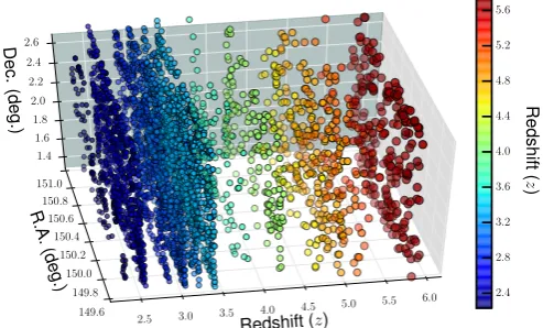
Figure 4.The 3D distribution of the SC4K sample presented in this paper in the full 2 deg2_{COSMOS field (see TableA1),}

show-ing all LAEs from the 16 different redshift slices, colour coded by redshift (blue to red from lower to higher redshift). The red-shift is computed using the central wavelength of the medium-or narrow-band filter. SC4K probes roughly 4,000 LAEs selected over a total volume close to∼108_Mpc3_{(see Table4for volumes}

probed per filter).

fromMU V =−19.2±0.2 for our lowest redshift sample (the deepest in Lyα) to up toMU V ∼ −21 at higher redshift (see Paulino-Afonso et al. 2017a).

3.7 Final sample: SC4K

Our sample of medium-band selected LAEs consists of 3434 sources (see Table3), visually inspected for spurious detec-tions. We complement our medium-band LAEs with four narrow-band studies (Table3) in the COSMOS field which follow the same methodology as in this paper. We add 159 LAEs atz_∼2.23 (CALYMHA survey;Sobral et al. 2017b) and 45 sources atz ∼3.1 (Matthee et al. 2017b), selected with narrow-bands NB392 and NB501. In addition, we also include 78 LAEs at z ∼ 4.8 (Perez et al. in prep) and 192 LAEs at z _∼ 5.7 (Santos et al. 2016), selected with the narrow-bands NB711 and NB816, respectively. Our final sample of LAEs contains 3908 sources. We name this sample of _∼4,000 (4k) LAEs, obtained by “slicing” the COSMOS field (Figure 4), as SC4K. For an example and description of the catalogue, see TableA1. Our survey is roughly equiv-alent to a very wide, low resolution (R ∼ 20−80) IFU Lyαsurvey covering all the way from z _∼2.2 toz _∼6. A 3D view (showing the full COSMOS field and redshift as a depth dimension) of SC4K is shown in Figure4.

4 METHODS AND CORRECTIONS

4.1 Lyαluminosities and survey volumes

We compute Lyα luminosities for each of our LAE candi-dates per filter/redshift slice by using i) their estimated Lyα

fluxes in 200apertures (FLyα; see e.g.Sobral et al. 2017b) and ii) the luminosity distance (DL) corresponding to Lyαlines detected at the central wavelength of each filter. Luminos-ity distances (DL) range from 20×103Mpc atz ≈2.5 to

Table 4.The Lyαsurvey co-moving volumes per redshift/filter slice assuming top-hat filter profiles for medium- and narrow-band filters. We provide the filter name and the Lyα volume corre-sponding to the 50% transmission points in the normalised filter profile. The two final columns on the right present the limiting luminosity limit (log10LLyα/erg s−1) for each slice, by using the

formal flux limits from Table1and the 30% completeness limit that we measure with out methodology (see Section4.2.1).

Filter Area Volume LLyα,3σ LLyα30%

(deg2_{) (10}6_Mpc3_{) (log}

10) (log10)

IA427 1.94 4.0 42.4 42.5

IA464 1.94 4.2 42.5 42.9

IA484 1.94 4.3 42.5 42.7

IA505 1.94 4.3 42.6 42.7

IA527 1.94 4.5 42.5 42.7

IA574 1.96 4.9 42.7 43.0

IA624 1.96 5.2 42.8 42.9

IA679 1.96 5.5 43.0 43.1

IA709 1.96 5.1 42.9 43.1

IA738 1.96 5.1 43.0 43.3

IA767 1.96 5.5 43.0 43.4

IA827 1.96 4.9 43.0 43.4

NB392 1.21 0.6 42.3 42.3

NB501 0.85 0.9 42.9 43.0

NB711 1.96 1.2 42.6 42.9

NB816 1.96 1.8 42.5 42.5

Total 1.96 61.5 42.4-43 42.5-43.4

55_×103_{Mpc atz}

≈5.8. Lyαluminosities are then calculated as LLyα = 4πFLyαD2L. We find that our “formal” 3σ limit MB detections correspond to Lyαluminosity limits ranging from 1042.4_{erg s}−1_{atz= 2.5 to 10}43.0_{erg s}−1_{atz= 5.8 (see}

Table4for luminosity limits per filter).

Paulino-Afonso et al.(2017a) measured the rest-frame UV sizes of our LAEs, concluding they have half-light-radii in the range_≈0.1₋0.200_{(≈0.7−1.3 kpc), and thus} signif-icantly smaller than our 200apertures. However, due to the use of ground-based imaging (with a larger PSF) and the fact that we are tracing Lyαand not the rest-frame UV, the 200apertures may be missing some flux. We thus study how the fluxes computed in 200_{apertures compare with fluxes} de-rived from using an estimate of the full flux using e.g. mag-auto. We find an average ratio (Flux[mag−auto]/Flux[200_]) of ≈1.03±0.26 (median of 1.02). There is no systematic dif-ference in our sample as a whole nor any significant trend with redshift. Therefore, in this study we do not apply any further aperture correction and base our measurements on our directly measured 200_{aperture quantities (see discussion} inDrake et al. 2017b).

We compute the co-moving volumes probed by each of the medium-bands by approximating them to top-hat filters (using the measured FWHM; Table1). We find co-moving volumes within (4.0−5.5)×106Mpc3 per medium-band and a total co-moving volume of 5.7_×107_Mpc3 _{over all}

12 medium-bands; see Table4. The sum of all narrow-band volumes contributes with a modest volume of 4.5_×106_Mpc3_,

6.2×107Mpc3. We note that while our survey is only sen-sitive to the more typical and bright Lyαemitters, it pro-vides a unique opportunity to explore the bright end of the Lyαluminosity function mostly for the first time, being fully complementary to other previous surveys. For example, we probe a volume _≈50,000 times larger than MUSE (Drake et al. 2017a) and _≈ 50₋60 times the volumes of typical 1 deg2 narrow-band surveys (Ouchi et al. 2008) and still a factor of a_∼2₋3 larger than current_∼10₋20 deg2_surveys

with Hyper-Suprimecam (e.g.Konno et al. 2017).

4.2 Corrections to the Lyαluminosity function

4.2.1 Completeness correction

Sources with weak emission lines or with low EWs may be missed by our selection criteria, causing the measured num-ber density of sources to be underestimated. To estimate the line flux completeness we followSobral et al.(2013), adapted for Lyα studies byMatthee et al. (2015). Briefly, for each medium-band we obtain a sample of non-emitters at the red-shift we intend to study from the appropriate MB catalogue. To do so, we use the sources which are not classified as line-emitters (we exclude the line-line-emitters) and, from these, we select sources which are consistent with being at a redshift ±0.2 of the Lyα redshift for a given filter. We do this by i) applying the same Lyman break selection as we did for the sample of line-emitters and ii) by selecting sources with photometric redshifts within_±0.2 (Laigle et al. 2016) of the redshift window shown in Table3. We check that our method leads to a distribution in MB magnitudes of non-emitters in agreement with that of the LAEs, with a tail of _∼2₋5% brighter sources. Overall, our empirical approach leads to a sample of non-line emitters that is slightly brighter than that of LAEs, and thus can be seen as a conservative approach in estimating completeness corrections that does not require making any assumptions to create fake/mock sources.

Our procedure results in samples of non-line-emitters per MB filter that are at roughly the same redshift as our LAEs and allow us to estimate our line-flux completeness with an empirical/data approach. To do so, we add emis-sion line flux to sources in steps of 10−18_{erg s}−1_cm−2_{, which}

results in increasing the flux of the medium- and broad-bands depending on the filter’s FWHM. For each step in flux added, we apply our emission-line selection criteria and identify those that, with the flux added, now make it into a new sample of line emitters and compare those with the total sample that was flux-boosted. By determining the frac-tion that we retrieve (after applying our Σ and EW cuts; see Section3.1) as a function of added line-flux in comparison with the full sample, we obtain a completeness estimation for each flux, which we apply to our luminosity functions. We only calculate the Lyαluminosity function for luminos-ity bins in which we find a completeness of 30% or higher at the lowest luminosity limit of the bin; these are in the range LLyα = 1042.5−43.4erg s−1 (see Table 4). Our lowest luminosity bin is the one affected by the largest incomplete-ness and thus the one with the highest completeincomplete-ness cor-rection being applied, which is typically a factor of≈2. We find that the completeness functions strongly depend on line flux, with completeness typically growing from 30% to 90%

42.5 42.7 42.9 43.1 43.3 43.5 43.7

log

(L

/erg s

)

0.5 0.6 0.7 0.8 0.9 1.0

output

,

filter

profile

/

input

,

Sc

hec

hter

IA827 medium-band filter (S-cam) NB816 narrow-band filter (HSC)

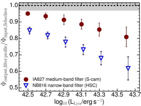
Figure 5.The observed ratio between 10,000 observed Lyα lu-minosity functions using the real filter profiles and a Schechter input simulated sample of LAEs assuming tophat filters. Our re-sults highlight the need to correct for filter profile effects which pushes sources from intrinsically bright to observed fainter bins, and highlights that the corrections are particularly important for narrow-band surveys, but are still relevant for medium-band sur-veys.

in_≈0.4₋0.5 dex increases in Lyαluminosity, and reaching ≈100% with a further∼0.5 dex increase.

4.2.2 Filter profile effects and corrections

As discussed in detail in e.g.Sobral et al.(2013) andMatthee et al.(2015), due to the non-top-hat shape of narrow-band filters, sources can be observed at a low transmission (al-most no source is observed at full transmission when a filter is well described by a Gaussian function), particularly once survey volumes are large. As a result, assuming a top-hat fil-ter will cause a complex underestimation of the flux, which is manifested in the luminosity function as a transfer of in-trinsically bright sources towards observed fainter sources. For an intrinsic Schechter distribution, and particularly for the exponential regime (bright end), this effect results in an underestimation of the number density of the brightest emit-ters (as they can only be detected as bright over a small red-shift range corresponding to the filter’s peak transmission), and sometimes an overestimation of the faintest sources (as brighter sources detected away from peak transmission will look fainter). However, the necessary corrections depend on i) the filter profile, ii) the intrinsic shape of the luminosity function and iii) the depth and survey volumes.

While medium-bands are broader than narrow-bands and in general better fitted by a top-hat, a full investigation of the role of the filter profiles is still required. We estimate potential corrections for each filter by simulating ten million sources with an input random redshift distribution6_{which is} wide enough to cover down to zero transmission by each fil-ter on the blue and red wings. We generate these ten million sources with a luminosity distribution given by the observed

6 _{Note that the output distribution is not random and follows}

(completeness corrected) luminosity function, following So-bral et al. (2013). By convolving the full population with i) the real filter profile and ii) the top-hat approximation we can determine the number density ratio between i) and ii) per luminosity and derive corrections based on the filter profile; an example for IA827 and the NB816 (from HSC) filters is shown in Figure5(see also FigureC1).

Our results show that the use of medium-band filters results in smaller corrections (see also AppendixC1) than those derived for typical narrow-band filters (Figure5). This is because fluxes are only significantly underestimated at the wings of the medium-band filters, which correspond to a much smaller fractional volume than for narrow-band filters. We also note that the input shape of the luminosity func-tion is crucial for the estimated filter profile effect: while an observed Schechter function leads to a large correction in the exponential part, a bright end which is observationally described by a much slower decline with luminosity (e.g. a power-law with a shallow slope) results in smaller correc-tions (see full discussion in AppendixC1). Our results thus mean that while for previous deep surveys mostly tracing the faint-end power-law component of the Schechter func-tion the correcfunc-tions could be relatively small, for the bright end (under a Schechter assumption) the corrections can be large, close to a factor of 2-3 for narrow-band filters at the highest luminosities, while they can be a factor of 1.2-1.3 for medium-bands (see FigureC1).

While the filter profile effects can be small for medium-bands, we still take them into account by applying a statis-tical correction to each luminosity bin. This produces our final luminosity function (LF). We provide a more detailed analysis and discussion of the effects, assumptions and cor-rections due to the various filter profiles when contrasted to top-hat approximations in AppendixC1. We also note that indirect statistical tests for our corrections can be obtained when comparing our results with e.g. MUSE (Drake et al. 2017b) and other IFU surveys which are not affected by filter profile effects (see Section5.1).

4.3 Flux robustness and errors: random and systematic

Due to errors in the photometry, both in the MB and BB magnitudes, estimated Lyαfluxes will be subject to errors and, in some cases, also prone to potential systematic ef-fects. We study these errors and their potential role in the derivation of the LyαLF. Briefly, we assume that each MB and BB magnitudes and their uncertainties are described by normal distributions centred on the measured value and with the width that is equal to its associated 1σ error. We then perturb each galaxy magnitude 10,000 times by ran-domly picking values from their individual probability dis-tributions. We use these perturbed magnitudes to compute the LyαLF. We do not find any systematic difference, show-ing that the errors on the MB and BB photometry have no systematic effect in our methodology. We use the difference between the median value and the 16th and 84th percentiles of the perturbed number density distribution as the lower and upper errors on the number density for each luminosity bin. We find small variations due to this effect, with a median error of _≈0.03 error in log₁₀(Φ). This is particularly sub-dominant when compared to other sources of uncertainty,

42.5 42.7 42.9 43.1 43.3 43.5 43.7 43.9 Observed log10(LLy↵/erg s 1)

-0.5 -0.4 -0.3 -0.2 -0.1 0.0 0.1 0.2

Error

in

log

10

(

/Mpc

3)d

lo

gL

1

IA427 (z=2.5)

Poissonian error + Selection error + Completeness correction + Filter profile correction + Flux error correction

Figure 6.An example of the different error contributions to the Lyαluminosity bins from different sources of uncertainty which are taken in series in our analysis. We show bins with bin widths that increase with increasing Lyαluminosity. These include: Pois-sonian, perturbations to the selection criteria (from line emitters to LAEs; see Table3), line flux completeness, filter profile correc-tions and flux errors. We find that selection perturbation errors are most important at the faintest luminosities, but they still contribute to the brightest bins.

but we still add it (0.03 dex) at the end in quadrature (see Figure6).

4.4 Completeness-contamination errors in the LAE selection and final errors

While the flux and EW selection/limits can be taken into account for corrections and accounted for in errors (see Sec-tion4.2.1), there are other sources of uncertainties that are linked with the photometric or colour-colour criteria applied to select LAEs/filter lower redshift sources (Section 3.3). While no single cut is perfect (even more so due to pho-tometric errors), it is possible to perturb the selection and conduct a Markov chain Monte Carlo (MCMC) analysis in order to estimate the effects of varying the selection in the derivation of the LyαLF and propagated quantities. Here we implement such an analysis. We perturb the LAE selection criteria described in Table3in a i)±0.2 dex interval around each colour-colour and photometric cut, independently and ii) by randomly varying by+0.31

−0.44the 3σmagnitudes

(corre-sponding to varying non-detection limits in the range 2−4σ, from the least to the most conservative cuts) of bands trac-ing bluer of the Lyman-limit, used to reject interlopers. We run a MCMC simulation, with 10,000 iterations for each fil-ter, randomly picking sets of values inside the full explored range, assuming all have an equal probability (flat prior). We then calculate the selection criteria errors as the difference between the median value and the 16th and 84th percentiles within each luminosity bin for all realisations.

An example of the estimation of the full errors affecting log10(Φ) can be found in Figure6forz= 2.5 (IA427). We

bins where the Poissonian errors are very small (see Fig-ure6). The errors from perturbing the selection criteria are roughly a factor of up to 2.5 the Poissonian error per bin at the bins probing the faintest luminosities (with the largest number of sources), while they can be as low as 0.2-0.8 of the Poissonian errors if the bin is populated with only 5-10 sources (where the Poissonian error is already large). We also find that perturbation errors are more important (larger) at

z _∼2.5₋2.8 andz >4 than they are at z_∼3₋3.3. This roughly coincides with jumps in the selection criteria and whenever different colours/bands are used (see Table3).

We add our estimated perturbation errors in quadrature to the Poissonian errors, noting that they are particularly important for the faint end where the Poissonian errors are an underestimation of the full uncertainties. We then scale the errors by the line flux completeness correction and the filter profile correction, which we assume we know with 30% accuracy (and thus add an extra 30% of such corrections to the errors, taking a conservative approach). We note that we do not add any errors due to cosmic variance, but that given the very large volumes and the multiple redshift slices, we expect these to be just a small fraction of our full er-rors that are much larger than the formal Poissonian erer-rors. Finally, even though our samples are expected to be con-taminated by interlopers at the 10-15% level, similarly to other narrow-band surveys, our LAE selection-completeness implies we may be missing 10-15% of real LAEs (when we transform the sample of line emitters into candidate LAEs), and thus in our analysis we do not apply any corrections for this contamination or completeness, as they should roughly cancel out.

4.5 Redshift binning

Our multiple redshift slices allow to trace LAEs across well defined cosmic times fromz_∼2 toz_∼6. We can also com-bine the slices to produce a global LyαLF or obtain slightly broader redshift slices which are populated by a much larger number of sources, and that overcome even more cosmic vari-ance. We bin all our z _∼2.5₋6 slices (IA427 through to IA827) in order to produce a global high redshift LF and compare it with similar measurement made with the MUSE instrument (e.gDrake et al. 2017b) or with slit observations (e.g. Cassata et al. 2011). We also split the sample into 5 different redshift bins in the following way:

• z_∼2.2 (z= 2.22_±0.02; NB392) • z∼2.5 (z= 2.5±0.1; IA427)

• z_∼3.1 (z= 3.1_±0.4; IA464, IA484, IA505, IA527) • z∼3.9 (z= 3.9±0.3; IA574, IA624)

• z_∼4.7 (z= 4.7_±0.2; IA679, IA709) • z∼5.4 (z= 5.4±0.5; IA738, IA767, IA827)

When producing redshift binned LFs, we only use the volumes associated with a given medium-band if that spe-cific filter provides the necessary depth for a completeness above 30%.

4.6 Schechter, power-law and combined fits

The Schechter function (Schechter 1976) is a widely used parametrization of the LF, defined by three parameters:

the power-law slope α, the characteristic number density Φ? _{and the characteristic luminosity L}?_{. Observations up} to extremely low luminosities are necessary to accurately constrain the power-law slope α (e.g Dressler et al. 2015; Drake et al. 2017b). Our medium-bands cover “typical” lu-minosities and higher, thus not probing much fainter than L?_{, and do not allow to measureαon their own. However,} several studies have been able to obtain good constraints onαfromz _∼2 toz _∼6 (e.g.Dressler et al. 2015;Drake et al. 2017b;Santos et al. 2016;Konno et al. 2016), which has been shown to be very steep (<₋1.5) and potentially varying fromα≈ −1.7 atz= 2.2 (Konno et al. 2016;Sobral et al. 2017b) to α_{≈ −}2 (or even steeper; seeDrake et al. 2017b) by z _∼6 (Dressler et al. 2015; Santos et al. 2016; Drake et al. 2017b). We therefore fit Schechter functions by fixing/varyingαbetween₋1.6 and₋2.0, but we also explore fits withα fixed to−1.8 at all redshifts in order to inves-tigate the potential redshift evolution of L?

Lyα and Φ∗Lyα at fixedα. Finally, we also fit α explicitly by combining our results with ultra-deep observations.

In addition to fitting Schechter functions, we also fit power-laws of the form log10Φ =Alog10LLyα+B to the full LFs and compare these with Schechter fits. Finally, we also explore combinations of a Schechter for lower luminosi-ties and a power-law at higher luminosiluminosi-ties when a single function yields a very bad fit on its own (see Section5). For all LFs, we follow a MCMC approach for the fits, perturb-ing each bin independently within its asymmetric Gaussian error probability distribution and fitting for 10,000 re-alisations per LF. We take the median of all the best fits as the most likely combination of parameters and estimate the errors by computing the 16th and 84th percentiles for all 10,000 realisations per LF estimation. We note that due to degeneracies in the parameters, these errors can some-times exaggerate the errors on individual parameters (i.e., parameters are linked and only allowed to vary within some specific relation and not independently), but they are gener-ally well constrained. For each best-fit we also compute the correspondingχ2

redand use these to obtain the medianχ2red

and the 16th and 84th percentiles of all realisations.

4.7 X-ray and radio properties: AGN candidates within our LAEs

41.0 41.5 42.0 42.5 43.0 43.5 44.0 44.5 45.0

Observed log

10

(L

Lyα

/erg s

−

1

)

-8.0

-7.0

-6.0

-5.0

-4.0

-3.0

-2.0

-1.0

log

10

(

Φ

/Mpc

−

3

)d

lo

gL

−

1

α

=

−

1

.

93

log

Φ

=

−

3

.

45

log

L

= 42

.

93

S-SC4K

L

Lyα

SC4K

(2.5

<

z

<

6)

2.9< z <6.6(Drake+17a) 2.9< z <6.6(Drake+17b) 3.0< z <6.5(Bina+16) 2.0< z <3.0(Cassata+11) 3.0< z <4.6(Cassata+11) 4.6< z <6.6(Cassata+11)

All LAEs (SC4K) Removing X-ray+Radio X-ray+Radio LAEs only Power-law fit (bright-end)

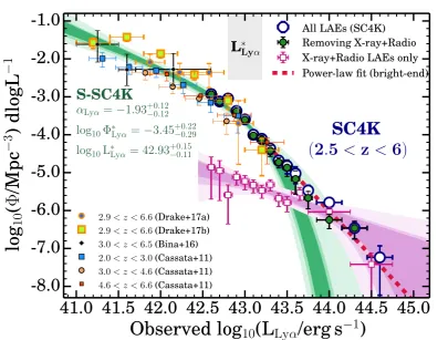
Figure 7.The combined global LyαLF at 2.5 < z <6. Our large samples of luminous LAEs, obtained over a co-moving volume of 0.6×108_Mpc3 _{are able to constrain the bright end of the LyαLF for the first time down to number densities of∼10}−7_Mpc−3 _and

Lyαluminosities of∼1044.5_{erg s}−1_{. We find a significant excess of bright LAEs at the highest luminosities when compared to a single}

Shechter function and show that is likely driven by a population where Lyα is AGN-driven. We compute a proxy for the AGN Lyα

LF with X-ray and radio AGN among our sample (1 and 2σ contours shown for Schechter function fits). We also compare our results with recent MUSE/VLT (Bina et al. 2016;Drake et al. 2017a,b) and VIMOS/VLT observations (e.g.Cassata et al. 2011), showing a very good agreement in the L∗

Lyαrange where all studies overlap. Deeper, smaller volume studies from the literature allow to cover the

sub-L?

Lyαluminosity regime, being perfectly complementary to our approach. Overall, we show the LyαLF determined over 4 orders of

magnitude in Lyαluminosity and 6 orders of magnitude in number densities atz∼2.5−6 resulting in the ‘synergy’ LyαLF (S-SC4K; 2.5< z <6) and the 1, 2 and 3σconfidence levels when fitting a Schechter function up to 1043.3_{erg s}−1_{(we also show the power-law fit}

done for higher luminosities). Results are provided in Table5.

for redshifts 2.7< z <3.5 and 3.5< z <6, respectively. We also identify a clear relation between the X-ray AGN frac-tion and Lyαluminosity of LAEs (see Calhau et al. 2018), qualitatively similar to what has been found at lower red-shift (Wold et al. 2014,2017) and also found and discussed inOuchi et al.(2008) andMatthee et al.(2017b).

In the VLA radio data (1.4 GHz and 3 GHz; see Schin-nerer et al. 2010;Smolˇci´c et al. 2017) we identify 62 indi-vidual sources, with these being dominated by the 3 GHz detections (61), and we class these as AGN. Out of these, 30/62 are also X-ray sources. We therefore find a total of 141 AGN sources among the SC4K sample of LAEs, yielding a total AGN fraction of 3.6_±0.3%. If we split the sample in three redshift ranges, we find that the AGN fraction slowly declines from z _∼2.2₋2.7 (4.7_±0.7%) to z _∼ 2.7₋3.5 (4.4±0.4%) and then drops significantly at z ∼ 3.5−6 (1.2_±0.4%). Concentrating on radio AGN within our sample of LAEs, we find that the (radio) AGN fraction is relatively constant (1.9_±0.4%) at z _∼ 2.2₋3.5 and then drops to 0.9_±0.2% atz_∼3.5₋6.

5 RESULTS

5.1 The global LyαLF at z_∼2.5₋6

In Figure7 we present the global LyαLF at z ∼2.5−6, determined with a total volume of close to _∼ 108_Mpc3_.

Our results probe Lyα luminosities from _∼ 1042.5_{erg s}−1

to∼ 1044.5_{erg s}−1_{, covering 2 orders of magnitude in Lyα}

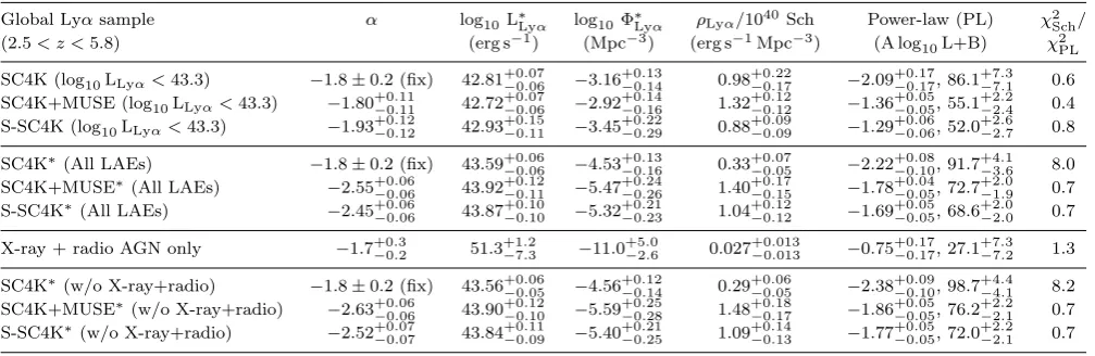
luminosity with a single survey. Down to our observational limits, we find that the global LyαLF atz∼2.5−6 resem-bles a single or double power-law (or a double Schechter, but not a single Schechter function) and extends to lumi-nosities and number densities that reach into what is ex-pected from the quasar luminosity function (e.g. Richards et al. 2006) and follow-up of quasars in Lyα(e.g.Borisova et al. 2016). Fitting the global SC4K Lyα LF leads to a power-law of −2.22+0₋₀._.08₁₀log₁₀(LLyα) + 91.7+4₋3..16 (see Table

5), which describes the data significantly better than a sin-gle Schechter function (χ2Sch/χ2PL ≈ 8; see Table5). If we