Geometric Representations of Random Hypergraphs

Geometric representations of random hypergraphs

Abstract

We introduce a novel parametrization of distributions on hypergraphs based on the geom-etry of points inRd. The idea is to induce distributions on hypergraphs by placing priors on point configurations via spatial processes. This prior specification is then used to infer condi-tional independence models or Markov structure for multivariate distributions. This approach supports inference of factorizations that cannot be retrieved by a graph alone, leads to new Metropolis-Hastings Markov chain Monte Carlo algorithms with both local and global moves in graph space, and generally offers greater control on the distribution of graph features than currently possible. We provide a comparative performance evaluation against state-of-the-art, and we illustrate the utility of this approach on simulated and real data.

Keywords: Abstract simplicial complex, Computational topology, Copulas, Factor models, Graphical models, Random geometric graphs.

Contents

1 Introduction 1

1.1 Related work . . . 1

1.2 Contributions . . . 2

2 Background and preliminaries 3 2.1 Graphical models . . . 3

2.2 Geometric graphs . . . 5

2.3 Random geometric graphs . . . 10

3 Geometric representations of random hypergraphs 11 3.1 Prior specifications . . . 12

3.2 Sampling from prior and posterior distributions . . . 13

3.2.1 Prior sampling . . . 14

3.2.2 Posterior sampling . . . 15

3.3 Convergence of the Markov chain . . . 15

4 Results 16 4.1 Illustration of modeling advantages . . . 16

4.1.1 The nerve determines the junction tree factorization . . . 16

4.1.2 Subgraph counts in RGGs are a function ofQ . . . 17

4.2 Simulation studies . . . 20

4.2.1 Gis in the Space Generated byA . . . 20

4.2.2 Gaussian graphical model . . . 22

4.2.3 Factorization Based on Nerves . . . 24

4.2.4 GOutside the Space Generated byA . . . 28

4.3 Comparative performance analysis with state-of-the-art . . . 30

4.3.1 Scalability . . . 33

4.4 Real data analysis . . . 34

4.4.2 Daily exchange rates data . . . 36

5 Discussion 36

A Filtrations and Decomposability in Random Geometric Graphs 42

A.1 Example . . . 43

1

Introduction

Consider the problem of making inference on the dependence structure among random variables

X1, ..., Xp ∈Rp, frommreplicated observations. The dominant formalism for this problem, is that

of graphical models (Lauritzen, 1996). In this formalism. the focus is on the first two moments

of the observation vector,X ={X1, ..., Xp}, and the dependence structure is specified in terms of

pairwise relations, which define an undirected graph. If such a graph is decomposable, inference is

typically carried out efficiently. Here we detail a new approach for the construction of distributions

on undirected graphs, motivated by the problem of Bayesian inference of the dependence structure

among random variables.

1.1

Related work

It is common to model the joint probability distribution of a family of p random variables

{X1, . . . , Xp}in two stages. First specify theconditional dependence structureof the distribution,

then specify details of the conditional distributions of the variables within that structure (seep. 1274

ofDawid and Lauritzen 1993, orp. 180 ofBesag 1975, for example). The structure may be summa-rized in a variety of ways in the form of a graphG = (V,E)whose verticesV ={1, ..., p}index the

variables{Xi}and whose edgesE ⊆ V × V in some way encode conditional dependence. We

fol-low the Hammersley-Clifford approach (Besag, 1974;Hammersley and Clifford, 1971), in which

(i, j) ∈ E if and only if the conditional distribution ofXi given all other variables{Xk: k6=i}

depends onXj, i.e., differs from the conditional distribution ofXi given{Xk : k 6=i, j}. In this

case the distribution is said to be Markov with respect to the graph. One can show that this graph

is symmetric orundirected,i.e., all the elements ofE are unordered pairs.

The simultaneous inference of a decomposable graph and marginal distributions in a fully

Bayesian framework was approached in (Green,1995) using local proposals to sample graph space.

A promising extension of this approach called Shotgun Stochastic Search (SSS) takes advantage

of parallel computing to select from a batch of local moves (Jones et al., 2005). A stochastic

search method that incorporates both local moves and more aggressive global moves in graph

space has been developed by Scott and Carvalho (2008). These stochastic search methods are

intended to identify regions with high posterior probability, but their convergence properties are

still not well understood. Bayesian models for non-decomposable graphs have been proposed by

Roverato (2002) and byWong, Carter, and Kohn (2003). These two approaches focus on Monte

Carlo sampling of the posterior distribution from specified hyper Markov prior laws. Their

em-phasis is on the computational problem of Monte Carlo simulation, not on that of constructing

efficient exploration of the model space and a simple and flexible family of distributions on graphs

that can reflect meaningful prior information.

Erd¨os-R´enyi random graphs (those in which each of the p₂ possible undirected edges (i, j)

is included inE independently with some specified probabilityα ∈ [0,1]), and variations where

the edge inclusion probabilities αij are allowed to be edge-specific, have been used to place

in-formative priors on decomposable graphs (Heckerman et al.,1995;Mansinghka et al.,2006). The

number of parameters in this prior specification can be enormous if the inclusion probabilities

are allowed to vary, and some interesting features of graphs (such as decomposability) cannot be

expressed solely through edge probabilities. Mukherjee and Speed(2008) developed methods for placing informative distributions on directed graphs by usingconcordance functions(functions that

increase as the graph agrees more with a specified feature) as potentials in a Markov model. This

approach is tractable, but it is still not clear how to encode certain common assumptions within

such a framework.

For the special case of jointly Gaussian variables {Xj}, or those with arbitrary marginal

dis-tributions Fj(·) whose dependence is adequately represented in Gaussian copula form Xj = F_j−1 Φ(Zj)

for jointly Gaussian {Zj} with zero mean and unit-diagonal covariance matrix C,

the problem of studying conditional independence reduces to a search for zeros in the precision

matrixC−1_{. This approach (see Hoff, 2007, for example) is faster and easier to implement than}

ours in cases where both are applicable, but is far more limited in the range of dependencies it

allows. For example, a three-dimensional model in which each pair of variables is conditionally

independent given the third cannot be distinguished from a model with complete joint dependence

of the three variables (we return to this example in Section4.2.3).

1.2

Contributions

In this article we establish a novel approach to parametrize spaces of graphs. For any inte-gers p, d ∈ _N, we show in Section 2.2 how to use the geometrical configuration of a set {vi}

of p points in Euclidean space _Rd _{to determine a graph G = (V,E) on V = {v}

1, ..., vp}. Any

prior distribution on point sets{vi}induces a prior distribution on graphs, and sampling from the

posterior distribution of graphs is reduced to sampling from spatial configurations of point sets—

a standard problem in spatial modeling. Relations between graphs and finite sets of points have

arisen earlier in the fields of computational topology (Edelsbrunner and Harer,2008) and random

geometric graphs (Penrose, 2003). From the former we borrow the idea ofnerves, i.e., simplicial

complexes computed from intersection patterns of convex subsets ofRd; the1-skeletons (collection

As a side benefit our approach also yields estimates of the conditional distributions given the

graph. The model space of undirected graphs grows quickly with the dimension of{X1, . . . , Xp}

(there are 2p(p−1)/2 _{undirected graphs on p vertices) and is difficult to parametrize. We propose}

a novel parametrization and a simple, flexible family of prior distributions on G and on Markov probability distributions with respect to G (Dawid and Lauritzen, 1993); this parametrization is

based on computing the intersection pattern of a system of convex sets in_Rd_{. The novelty and main}

contribution of this paper is structural inference for graphical models, specifically, the proposed

representation of graph spaces allows for flexible prior distributions and new Markov chain Monte

Carlo (MCMC) algorithms.

From the random geometric graph approach we gain understanding about the induced

distribu-tion on graph features when making certain features of a geometric graph (or hypergraph)

stochas-tic.

2

Background and preliminaries

2.1

Graphical models

The graphical models framework is concerned with the representation of conditional

dependen-cies for a multivariate distribution in the form of a graph or hypergraph. We first review relevant

graph theoretical concepts and then relate these concepts to factorizing distributions.

AgraphGis an ordered pair(V,E)of a setV ofverticesand a set E ⊆ V × V ofedges. If all

edges are unordered (resp., ordered), the graph is said to beundirected(resp.,directed). All graphs

considered in this paper are undirected, unless stated otherwise. Ahypergraph, denotedH, consists

of a vertex setV and a collectionKof unordered subsets ofV (known ashyperedges); a graph is

the special case where all the subsets are vertex pairs. A graph iscompleteifE =V × Vcontains

all possible edges; otherwise it isincomplete. A complete subgraph that is maximal with respect to inclusion is aclique. Denote byC(G)andQ(G), respectively, the collection of complete sets and

cliques ofG. Apathbetween two vertices{vi, vj} ∈ V is a sequence of edges connectingvi tovj.

A graph such that any pair of vertices can be joined by a unique path is atree. Adecomposition

of an incomplete graphG = (V,E)is a partition ofV into disjoint nonempty sets(A, B, S)such

that S is complete in G andseparates A and B, i.e., any path from a vertex in A to a vertex in

B must pass throughS. Iterative decomposition of a graphG such that at each step the separator

Si is minimal and the subsetsAi andBi are nonempty generates theprime componentsof G, the

collection of subgraphs that cannot be further decomposed. If all prime components of a graph

whose vertices are its prime components P(G); this is called itsjunction treerepresentation. A

junction tree is a hypergraph.

Let P be a probability distribution on _Rp _{and X = (X}

1, . . . , Xp) a random vector with

dis-tribution P. Graphical modeling is the representation of the Markov or conditional dependence

structure among the components{Xi}in the form of a graphG= (V,E). Denote byf(x)the joint

density function of{Xi}(or probability mass function for discrete distributions— more generally,

density for an arbitrary reference measure). The distributionP (and hence its density f(x)) may

depend implicitly on a vectorθof parameters, taking values in some setΘG, which in some cases

will depend on the graphG; writeΘ = tΘGfor the disjoint union of the parameter spaces for all

graphs onV.

Each vertexvi ∈ V is associated with a variableXi, and the edgesE determine how the

distri-bution factors. The densityf(x)for the distribution can be factored in a variety of ways associated

with the graphG(Lauritzen,1996,p. 35). It may be factored in terms of complete setsa∈C(G):

f(x) = Y

a∈C(G)

φa(xa|θa), (2.1a)

or similarly in terms of cliques a ∈ Q (assuming f is positive, according to the

Hammersley-Clifford theorem); ifG is decomposable thenf(x)may also be factored in junction-tree form as:

f(x) =

Q

a∈P(G)ψa(xa |θa) Q

b∈_S(G)ψb(xb |θb)

, (2.1b)

where P(G) and S(G) denote the prime factors and separators of G, respectively, and where

ψa(xa |θa)denotes the marginal joint density for the componentsxafor prime factorsa ∈P(G)

and ψb(xb | θb) that for separators b ∈ S(G) (Dawid and Lauritzen, 1993, Eqn. (6)). In the

Gaussian case, a similar factorization to (2.1b) holds even for non-decomposable graphs (Roverato,

2002, Prop. 2).

The prior distributions required for Bayesian inference about models of the form (2.1) may

be specified by giving a marginal distribution on the set of all graphs G ∈ Gp on p vertices and

conditional distributions on eachΘG, the space of parameters for that graph:

p(G, θ) =p(G)p(θ| G), G ∈Gp, θ∈ΘG (2.2)

whereθ ∈ΘGdetermines the parameters{θa :a∈C(G)}or{θa :a∈P(G)}and{θb :b∈S(G)}.

(1993) offer a rigorous framework for specifying more general prior distributions onΘG. Such

pri-ors, calledhyper Markov laws, inherit the conditional independence structure from the sampling

distribution, now at the parameter level. The hyper Inverse Wishart, useful when the factors are

multivariate normal, is by far the most studied hyper Markov law. Most previously studied mod-els of the form (2.2) specify very little structure on p(G)(Giudici and Green, 1999; Heckerman

et al., 1995; Roverato, 2002)— typically p(G) is taken to be a uniform distribution on the space

of decomposable (or unrestricted) graphs, or perhaps an Erd¨os-R´enyi prior to encourage sparsity

(Mansinghka et al., 2006), with no additional structure or constraints and hence no opportunity to

express prior knowledge or belief.

Two inference problems arise for the model specified in (2.2): inference of the entire joint

posterior distribution of the graph and factor parameters,(θ,G), or inference of only theconditional

independence structure, which entails comparing different graphs via the marginal likelihood

Pr{G |x} ∝

Z

ΘG

f(x|θ,G)p(G)p(θ| G)dθ.

Inference aboutGmay now be viewed as a Bayesian model selection procedure (seeRobert,2001,

p. 348).

2.2

Geometric graphs

Most methodology for structural inference in graphical models either assumes little prior

struc-ture on graph space, or else represents graphs using high dimensional discrete spaces with no

obvi-ous geometry or metric. In either case prior elicitation and posterior sampling can be challenging.

In this section we propose parametrizations of graph space that will be used in Section 2.3 to

specify flexible prior distributions and to construct new Metropolis/Hastings MCMC algorithms with local and global moves. The key idea for this parametrization is to construct graphs and

hypergraphs from intersections of convex sets in_Rd_.

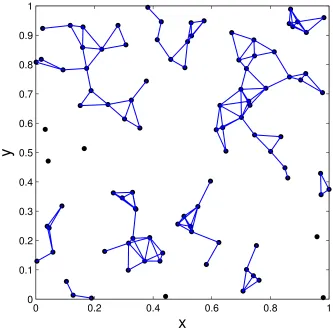
We illustrate the approach with an example. Fix a convex region A ⊂ _Rd _{and let V ⊂ A be}

a finite set of p points. For each number r ≥ 0, the proximity graph Prox(V, r) (see Figure 1)

is formed by joining every pair of (unordered) elements in V whose distance is 2r or less, i.e.,

whose closed balls of radius rintersect. As r ranges from0to half the diameter ofA, the graph Prox(V, r) ranges from the totally disconnected graph to the complete graph. This example is a

particular case of a more general construction illustrated in Figure2; hypergraphs can be computed

from properties of intersections of classes of convex subsets in Euclidean space. The convex sets

0 0.2 0.4 0.6 0.8 1 0

0.1 0.2 0.3 0.4 0.5 0.6 0.7 0.8 0.9 1

x

y

Figure 1: Proximity graph for100vertices and radiusr= 0.05.

Definition 2.1 (Nerve). Let F = {Aj, j ∈I} be a finite collection of distinct nonempty convex

sets. ThenerveofF is given by

Nrv(F) =

(

σ⊆I : \

j∈σ

Aj 6=_∅

) .

The nerve of a family of sets uniquely determines a hypergraph. We use the following three nerves

in this paper to construct hypergraphs (for more details, seeEdelsbrunner and Harer,2008).

Definition 2.2 ( ˇCech Complex). LetV be a finite set of points in _Rd and r > 0. Denote by _Bd the closed unit ball in _Rd. The Cech complexˇ corresponding toV and r is the nerve of the sets

Bv,r =v+r_Bd,v ∈ V. This is denoted by Nrv(V, r,Cechˇ ).

trian-gulationcorresponding toV is the nerve of the setsCv =x∈_Rd_{: kx−vk ≤ kx−uk, u∈ V}

forv ∈ V. This is denoted by Nrv(V,Delaunay), and the setsCv are calledVoronoi cells.

Definition 2.4 (Alpha Complex). Let V be a finite set of points in _Rd _{and r > 0. The Alpha}

complex corresponding to V and ris the nerve of the sets Bv,r ∩Cv, v ∈ V. This is denoted by

Nrv(V, r,Alpha).

−1 0 1

−1.5 −1 −0.5 0 0.5 1 1.5

x

y

−1 0 1

−1.5 −1 −0.5 0 0.5 1 1.5

x

y

−1 0 1

−1.5 −1 −0.5 0 0.5 1 1.5

x

y

−1 0 1

−1.5 −1 −0.5 0 0.5 1 1.5

x

y

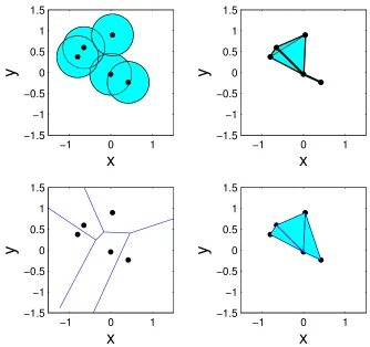
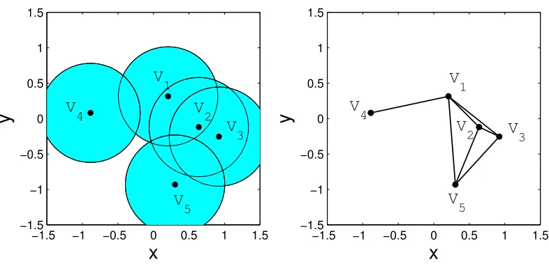
Figure 2: (a) A set of vertices inR2 are used to construct a family of disks of radiusr = 0.5. (b)

The nerve of this convex set. This is an example of a ˇCech complex. (c) For the same vertex set the Voronoi diagram is computed. (d) The nerve of the Voronoi cells is obtained. This is an example of the Delaunay triangulation. Note that the maximum clique size of the Delaunay is bounded by the dimension of the space of the vertex set plus one; such a restriction does not apply to the ˇCech complex.

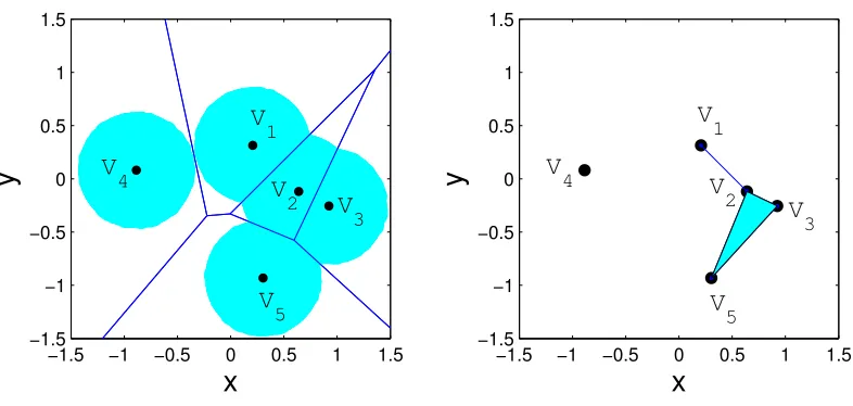
Here we illustrate the idea of nerve and specifically, the idea of alpha complex. Consider the

vertex set displayed in Table1andr= 0.5. The setsBv,r∩Cvand the corresponding nerve (alpha

complex) are illustrated in Figure3. Since the set indexed byV4 does not intersect with any other

−1.5 −1 −0.5 0 0.5 1 1.5 −1.5 −1 −0.5 0 0.5 1 1.5

x

y

−1.5 −1 −0.5 0 0.5 1 1.5 −1.5 −1 −0.5 0 0.5 1 1.5

x

y

5 V5

V

4

V

4

Figure 3: (a) Intersection of balls and Voronoi cells computed using r = 0.5and the vertex set listed in Table1. (b) The corresponding Alpha complex.

Coordinate V1 V2 V3 V4 V5

x 0.2065 0.6383 0.9225 −0.8863 0.3043

y 0.3149 −0.1193 −0.2544 0.0816 −0.9310

Table 1: Vertex set used for generating a family of sets and the corresponding nerve.

with the set indexed by V2, therefore there will be an edge joiningV1 andV2 in the nerve. V2, V3

andV5 intersect as pairs, therefore, the edges of the triangle with verticesV2, V3 andV5 will be in

the nerve. Since the sets indexed byV2,V3 andV5 also intersect as a triad, the facet or face of the

triangle is also included in the nerve.

The nerve of a family of sets is a particular class of hypergraphs known as (abstract) simplicial

complexes.

Definition 2.5(Abstract simplicial complex). LetV be a finite set. Asimplicial complexwith base

setV is a familyKof subsets ofV such thatτ ∈ Kandσ ⊆ τ impliesσ ∈ K. The elements ofK

are called simplices, and the number of connected components ofKis denoted](K).

The nerve of a collection of sets is always a hypergraph; in simple cases, only vertex pairs arise

so the1-skeleton determines a unique graph.

simplex τ ∈ K. Thep-skeletonof K is the collection of allτ ∈ K such that |τ| ≤ p+ 1. The

elements of thep-skeleton are calledp-simplices and the1-skeleton is just a graph (more precisely,

it isV ∪ E for a uniquely determined graphG = (V,E)).

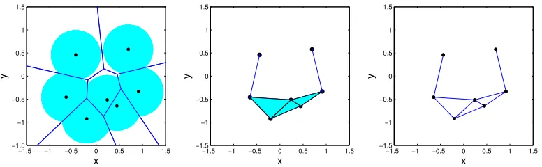
The 1-skeleton of a nerve is the graph obtained by considering only nonempty pairwise

inter-sections. The process of obtaining the nerve and the1-skeleton from a family of sets is illustrated

in Figure4. Different families of convex sets in_Rd_{induce different restrictions in graph space: for}

the Delaunay triangulation and the Alpha complex, for example, clique sizes cannot exceedd+ 1.

Although no such blanket restriction applies to the ˇCech complex, for this complex some graphs

are still unattainable— for example, no ˇCech complex can include a star graph whose central node

has degree higher than the “kissing number,”i.e., maximal number of disjoint unit hyperspheres

touching a given hypersphere, 6 ford= 2, 12 ford= 3,etc.

The ˇCech and Alpha complexes are hypergraphs indexed by a finite setV = {V1, . . . , Vp} ⊂

Rd and a size parameter r ≥ 0. Each induces a parametrization on the space of hypergraphs

(V, r) 7→ H(V, r). The classA of convex sets used to compute the nerve determines the space

of hypergraphs. To keep the notation simple,Awill be implicit whenever obvious by the context.

We will useA(V, r)to denote a generic element ofA for either the ˇCech or the Alpha complex.

Similarly,1-skeletons of nerves induce a parametrization of the spaces of graphs(V, r)7→ G(V, r).

Two principal advantages of this approach are:

1. For each family of convex sets{A}, the number of parameters needed to specify the graph

Gor hypergraphHgrows only linearly with the number of vertices;

2. The hypergraph parameter space will be a subset of_Rd_{, a very convenient parameter space}

−1.5 −1 −0.5 0 0.5 1 1.5

−1.5 −1 −0.5 0 0.5 1 1.5 x y

−1.5 −1 −0.5 0 0.5 1 1.5

−1.5 −1 −0.5 0 0.5 1 1.5 x y

−1.5 −1 −0.5 0 0.5 1 1.5

−1.5 −1 −0.5 0 0.5 1 1.5 x y

Figure 4: (a) Given a set of vertices and a radius (r = 0.5) one can computeAi =Ci ∩Bi, where Ciis the Voronoi cell for vertexiandBiis the ball of radiusrcentered at vertexi. (b) The Alpha

for MCMC sampling.

2.3

Random geometric graphs

In Section 2.2we demonstrated how the geometry of a set V ofppoints in_Rd _{can be used to}

induce a graphG. In this section we explore the relation between prior distributions onrandomsets

V of points in_Rd and features of the induced distribution on graphsG, with the goal of learning how to tailor a point process model to obtain graph distributions with desired features.

Definition 2.7 (Random Geometric Graph). Fix integersp, d ∈ _N and letV = (V1, . . . , Vp) be

drawn from a probability distributionQon(_Rd₎p_{. For any classAof convex sets in}

Rdand radius

r >0, the graphG(V, r,A)is said to be aRandom Geometric Graph(RGG).

While Definition2.7 is more general than that of (Penrose, 2003, p. 2), it still cannot describe

all the random graphs discussed in (Penrose and Yukich, 2001) (for example, those based onk -neighbors cannot in general be generated by nerves). For A we will use closed balls in _Rd _or

intersections of balls and Voronoi cells; most often Q will be a product measure under which

the{Vi}will bepindependent identically distributed (iid) draws from some marginal distribution

QM onRd, such as the uniform distribution on the unit cube[0,1]d or unit ball Bd, but we will

also explore the use of repulsive processes for V under which the points {Vi} are more widely

dispersed than under independence. It is clear that different choices forA,Qand rwill have an

impact on the support of the induced RGG distribution. To make this notion precise we define

feasible graphs.

Definition 2.8 (Isomorphic). Write G1 ∼= G2 for two graphs Gi = (Vi,Ei) and call the graphs

isomorphicif there is a 1:1 mappingχ: V1 → V2 such that(vi, vj) ∈ E1 ⇔ χ(vi), χ(vj)

∈ E2

for allvi, vj ∈ V1.

Definition 2.9 (Feasible Graph). Fix numbers d, p ∈ _N, a class A of convex sets in _Rd, and a distribution Qon the random vectors V in (_Rd₎p_{. A graph Γ is said to be feasible if for some}

numberr >0,

Pr{G(V, r,A)∼= Γ}>0.

In contrast to Erd¨os-R´enyi models, where the inclusion of graph edges are independent events,

the RGG models exhibit edge dependence that depends on the metric structure ofRdand the class Aof convex sets used to construct the nerves.

There is an extensive literature describing asymptotic distributions for a variety of graph

degree (for an encyclopedic account of results for the important case of1-skeletons of ˇCech

com-plexes, seePenrose, 2003). Several results for the Delaunay triangulation, some of which

gener-alize to the Alpha complex, are reported in (Penrose and Yukich, 2001). Regarding the support

on the distribution of hypergraphs induced by the complexes, generally, this is an area of open research (personal communication with H. Edelsbrunner). Recent work byKalhe(2014) surveys

some of this literature, focusing on random simplicial complexes. The monograph by Penrose

(2003) discusses the relationship betweenQand subgraph counts, the degree distribution, and the

percolation threshold, in Chapters 3, 4 and 10, respectively

Penrose(2003, Chap. 3) gives conditions which guarantee the asymptotic normality of the joint distribution of the numbersQjofj-simplices (edges, triads,etc.), foriidsamplesV = (V1, . . . , Vp)

from some marginal distributionQM onRd, as the numberp=|V|of vertices grows and the radius rp shrinks.

Simulation studies suggest that the asymptotic results apply approximately for p ≥ 24–100.

By this we mean that sometimes24is sufficient (the distribution of the vertices is approximately multivariate normal), and sometimes 100 may be required (distribution of the vertices far from

being multivariate normal).

3

Geometric representations of random hypergraphs

We develop a Bayesian approach to the problem of inferring factorizations of distributions of

the forms of (2.1),

f(x) = Y

a∈C(G)

φa(xa |θa) or Q

a∈P(G)ψa(xa|θa) Q

b∈_S(G)ψb(xb |θb)

.

In each case we specify the prior density function as a product

p(θ,G) = p(θ | G)p(G) (3.1)

of a conditional hyper Markov law forθ ∈Θand a marginal RGG law onG. We use conventional

methods to select the specific hyper Markov distribution (hyper Inverse Wishart for multivariate

normal sampling distributions, for example) since our principal focus is on prior distributions

for the graphs, p(G). Every time we refers to hyper Markov laws, it will be in the strong sense

according toDawid and Lauritzen(1993). We also present MCMC algorithms for sampling from

3.1

Prior specifications

All the graphs in our statistical models are built from nerves constructed in Section2.2from a

random vertex setV ={Vi}p_i=1 ⊂ _Rd_{and radiusr > 0. Since the nerve construction is invariant}

under rigid transformations (this is, transformations that preserve angles as well as distances) ofV

or simultaneous scale changes inV andr, restricting the support of the prior distribution onV to the unit ball_Bd_{does not reduce the model space:}

Proposition 3.1. Every feasible graph in _Rd may be represented in the form G(V, r,A) for a

collectionV ofppoints in the unit ball_Bdand forr = 1_p.

Proof. Let G = (V,E) ∼= G(V, r,A) be a feasible graph with |V| = p vertices. Every edge

(vi, vj)∈ E has length dist(vi, vj)≤2rso, by the triangle inequality, every connected component

ΓiofGwithpivertices must have diameter no greater than the longest possible path length,2r(pi−

1), and so fits in a ball Bi of diameter 2r(pi −1). The union of these balls, centered on a line

segment and separated byr(2 + 1/p), will have diameter less thanr(2p−1). By translation and linear rescaling we may taker = 1/pand bound the diameter by2, completing the proof.

We fixr= 1_p and simplify the notation by writingG(V,A)instead ofG(V, r,A)forA =Cechˇ orA =Alpha or, ifAis understood, simplyG(V). Thus we can induce prior distributions on the

space of feasible graphs from distributions on configurations ofppoints in the unit ball in_Rd.

Foriid uniform drawsV = (V1, . . . , Vp) fromBd, the expected number of edges of the graph

G(V, r,A)is bounded above byE[#E]≤ n₂

(2r)d_{; forr=} 1

p in dimensiond= 2this is less than

E[#E]<2, leading to relatively sparse graphs. We often take larger values ofr(still small enough for empty graphs to be feasible), to generate richer classes of graphs. A limit to how largermay

be is given by the partial converse to Prop.3.1,

Proposition 3.2. The empty graph on p vertices cannot be expressed as G(V, r,Cechˇ ) for any

V ⊂_Bd_{withr ≥ p}1/d₋₁−1_.

Proof. LetV ={V1, . . . , Vp} ⊂Bdbe a set of points andr >0a radius such thatG(V, r,Cechˇ )is

the empty graph. Then the ballsVi+rBdare disjoint and their union withd-dimensional volume pωdrdlies wholly within the ball(1 +r)Bdof volumeωd(1 +r)d(whereωd =πd/2/Γ(1+d/2)is

the volume of the unit ball), sop <(1 + 1_r)d_.

Slightly stronger, the empty graph may not be attained asG(V, r,Cechˇ )for anyr≥1/[(p/pd)1/d−

1]wherepdis the maximum spherical packing density inRd. Ford= 2, this gives the

3.2

Sampling from prior and posterior distributions

Let Q be a probability distribution on p-tuples in _Rd, p(G) the induced prior distribution on graphs G(V,Cechˇ ) for V ∼ Q with r = 1_p, and let p(θ | G) be a conventional hyper Markov law (see below). We wish to draw samples from the prior distributionp(θ,G)of (3.1) and from the

posterior distributionp(θ,G |x), given a vectorx= (x1, ..., xm)ofiidobservationsxj

iid

∼f(x|θ), using the Metropolis/Hastings approach to MCMC (Hastings, 1970; Robert and Casella, 2004,

Ch. 7).

We begin with a random walk proposal distribution in_Bdstarting at an arbitrary pointv ∈_Bd_,

that approximates the stepsV(0)_{, V}(1)_{, V}(2)_{, ... of a diffusionV}(t)_on

Bdwith uniform stationary

distribution and reflecting boundary conditions at the unit sphere∂_Bd_.

The random walk is conveniently parametrized in spherical coordinates with radius ρ(t) =k

V(t)kand Euler angles— ind=2dimensions, angleϕ(t)— at stept. Informally, we take indepen-dent radial random walk steps such that(ρ(t))dis reflecting Brownian motion on the unit interval (this ensures that the stationary distribution will beUn(_Bd_{)) and, conditional on the radius, angular}

steps from Brownian motion on thed-sphere of radiusρ(t)_.

Fix someη >0. Ind= 2dimensions the reflecting random walk proposal(ρ∗, ϕ∗)we used for step(t+ 1), beginning at(ρ(t), ϕ(t)), is:

ρ∗ =R[ρ(t)]2+ζ_ρ(t)η

1/2

, ϕ∗ =ϕ(t)+ζ_φ(t)η/ρ(t)

foriidstandard normal random variablesnζρ(t), ζ_φ(t) o

, where

R(x) =x−21₂(x+ 1)

is xreflected (as many times as necessary) to the unit interval. Similar expressions work in any

dimension d, with ρ∗ = R[ρ(t)_]d _+ζ(t) ρ η

1/d

and appropriate step sizes for the (d−1) Euler

angles.

For small η > 0this diffusion-inspired random walk generates local moves under which the proposed new point (ρ∗, ϕ∗) is quite close to (ρ(t)_{, ϕ}(t)_{) with high probability. To help escape}

local modes, and to simplify the proof of ergodicity below, we add the option of more dramatic

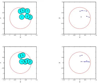
“global” moves by introducing at each time step a small probability of replacing(ρ(t)_{, ϕ}(t)_)with

a random draw(ρ∗, ϕ∗)from the uniform distribution on_Bd(see Figure5). Let q(V∗ _{| V)denote}

the Lebesgue density atV∗ _∈(

Bd)p of one step of this hybrid random walk forV = (V1, . . . , Vp),

−1.5 −1 −0.5 0 0.5 1 1.5 −1.5

−1 −0.5 0 0.5 1 1.5

x

y

−1.5 −1 −0.5 0 0.5 1 1.5 −1.5

−1 −0.5 0 0.5 1 1.5

x

y

−1.5 −1 −0.5 0 0.5 1 1.5 −1.5

−1 −0.5 0 0.5 1 1.5

x

y

−1.5 −1 −0.5 0 0.5 1 1.5 −1.5

−1 −0.5 0 0.5 1 1.5

x

y

Figure 5: This figure illustrates a global move. (a) The current configuration of the points. (b) The graph implied by this configuration. (c) The proposal configuration which is obtained by randomly moving one vertex. (d) The graph implied by the proposed move.

3.2.1 Prior sampling

To draw sample graphs from the prior distribution begin with V(0) _{∼ Q(dV) and, after each}

time step t ≥ 0, propose a new move to V∗ ∼ q(V∗ | V(t)). The proposed move from V(t) (with induced graphG(t) _{= G(V}(t)_{)) toV}∗ _(andG∗_{) is accepted (whereupon V}(t+1) _{= V}∗_{) with}

probability1∧H(t), the minimum of one and the Metropolis/Hastings ratio

H(t)= p(V

∗_{) q(V}(t) _|V∗₎ p(V(t)_)q(V∗ _|V(t)₎.

OtherwiseV(t+1) _{= V}(t)_{; in either case sett ← t+1 and repeat. Note the proposal distribution}

q(· | ·)leaves the uniform distribution invariant, soH(t) ≡ 1forQ(dV) ∝ dV and in that case

3.2.2 Posterior sampling

After observing a random sample X = x = (x1, . . . , xm) from the distribution xj ∼ f(x | θ,G), let

f(x|θ,G) =

m Y

i=1

f(xi |θ,G)

denote the likelihood function and

M(G) =

Z

ΘG

f(x|θ,G)p(θ| G)dθ (3.2)

the marginal likelihood forG. For posterior sampling of graphs, a proposed move fromV(t)_toV∗

is accepted with probability1∧H(t) _for

H(t) = M(G

∗_)p(V∗_{) q(V}(t)_|V∗₎

M(G(t)_)p(V(t)_)q(V∗ _|V(t)₎. (3.3)

For multivariate normal data X and hyper inverse Wishart hyper Markov law p(θ | G), M(G)

from (3.2) can be expressed in closed form for decomposable graphs G(V). efficient algorithms

for evaluating (3.2) are still available even if this condition fails.

The model will typically be of variable dimension, since the parameter spaceΘGfor the factors

may depend on the graphG=G(V). Not all proposed moves of the point configurationV(t) V∗ will lead to a change in G(V); for those that do we implement reversible-jump MCMC (Green,

1995;Sisson, 2005) using the auxiliary variable approach ofBrooks et al. (2003) to simplify the

book-keeping needed for non-nested movesΘG ΘG∗.

3.3

Convergence of the Markov chain

Denote byG˙(p, d,A)the finite set of feasible graphs withpvertices in_Rd_{,i.e., those generated}

from1-skeletons of A-complexes. For each G ∈ G˙(p, d,A) letVG ⊂ (_Bd₎p _{denote the set of all}

pointsV ={V1, . . . , Vp} ∈(Bd)p for whichG ∼=G(V,1_p,A), and setµ(G) =Q VG

. Then

Proposition 3.3. The sequenceG(t) _{= G(V}(t)_,1

p,A)induced by the prior MCMC procedure

de-scribed in Section 3.2.1 samples each feasible graph G ∈ G˙(p, d,A)with asymptotic frequency

µ(G). The posterior procedure described in Section3.2.2samples each feasible graph with

asymp-totic frequencyµ(G | x), the posterior distribution ofG given the dataxand hyper Markov prior

Proof. Both statements follow from the Harris recurrence of the Markov chain V(t) constructed in Section 3.2. For this it is enough to find a strictly positive lower bound for the probability of

transitioning from an arbitrary point V ∈ (_Bd₎p _{to any open neighborhood of another arbitrary}

pointV∗ ∈ (_Bd₎p _{(Robert and Casella, 2004, Theorem 6.38, pg. 225). This follows immediately}

from our inclusion of the global move in which allppoints{Vi}are replaced with uniform draws

from(_Bd₎p_.

It is interesting to note that while the sequenceG(t)_=G(V(t)_,1

p,A)is a hidden Markov process,

it is not itself Markovian on the finite state spaceG˙(p, d,A); nevertheless it is ergodic, by Prop.3.3.

4

Results

Here we illustrate the use of the proposed parametrization using simulations and real data.

These numerical examples provide us with an opportunity to test priors that encourage sparsity,

and MCMC algorithms that allow for local as well as global moves by design.

4.1

Illustration of modeling advantages

4.1.1 The nerve determines the junction tree factorization

Here we use a junction tree factorization with each univariate marginalXi associated to a point Vi ∈Rd(the standard graphical models approach). In this case, specifying the class of sets to

com-pute the nerve and the value forrdetermines a factorization for the joint density of{X1, . . . , Xp}.

We illustrate withp= 5points in Euclidean space of dimensiond= 2.

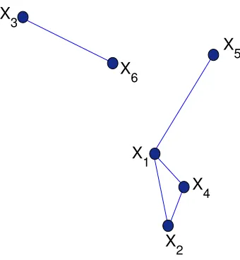
Let (X1, X2, X3, X4, X5) ∈ R2 be a random vector with densityf(x) and consider the vertex

set displayed in Table1(also shown as solid dots in Figures3and6).

For an Alpha complex withr = 0.5the junction tree factorization (2.1b) corresponding to the

graph in Figure3is

f(x) = ψ12(x1, x2)ψ235(x2, x3, x5)ψ4(x4)

ψ2(x2)

,

we will denote the factorization as [1,2][2,3,5][4]. In the case where the factors are potential

functions rather than marginals we will use{·}instead of[·]. Similarly, for the ˇCech complex and

r= 0.7the factorization corresponding to the graph in Figure6is

f(x) = ψ1235(x1, x2, x3, x5)ψ14(x1, x4)

ψ1(x1)

−1.5 −1 −0.5 0 0.5 1 1.5 −1.5 −1 −0.5 0 0.5 1 1.5

x

y

−1.5 −1 −0.5 0 0.5 1 1.5 −1.5 −1 −0.5 0 0.5 1 1.5

x

y

Figure 6: (a) ˇCech complex computed usingr = 0.7and the vertex set listed in Table1. (b) The

1-Skeleton of the ˇCech complex.

4.1.2 Subgraph counts in RGGs are a function ofQ

In this subsection we illustrate how the distribution of particular graph features changes as a

function of the sampling distribution of the random point setVand contrast this with Erd¨os-R´enyi

models. Specifically we will focus on the number of edges (2-cliques) Q2 and the number of

3-cliquesQ3.

The two spatial processes we study forQareiiduniform draws from the unit square[0,1]2 _in

the plane, and dependent draws from the Mat´ern type III hard-core repulsive process (Huber and

Wolpert, 2009), using ˇCech complexes with radiusr = 1/√150 ≈ 0.082 in both cases to ensure

asymptotic normality (Penrose, 2003, Thm. 3.13). In our simulations we vary both the number

of variables (graph size)pand the Mat´ern III hard core radius ρ. Comparisons are made with an

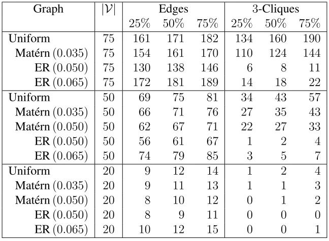
Erd¨os-R´enyi model with a common edge inclusion parameter. Table 2 displays the quartiles for

Q2 and Q3 as a function of the graph size p, hard core radius ρ, and Erd¨os-R´enyi edge inclusion

probabilityp. Figures7, 8, and9show the joint distribution of(Q2, Q3)for{Vi}

iid

∼ Un([0,1]2_),

for a Mat´ern III process with hard core radiusρ= 0.35, and for draws from an Erd¨os-R´enyi model

140 160 180 200 220 240 100

150 200 250 300 350 400 450

Edge Count

3−Clique Count

Figure 7: Edge counts and 3-Clique counts from 2,500 simulated samples of

G(V,1/√2·75,Cechˇ ) where |V| = 75 and Vi iid∼ Un([0,1]2), 1 ≤ i ≤ 75. The multivari-ate normal appears as a reasonable approximation for the joint distribution, as suggested by (Penrose,2003, Thm.3.13). ˇCech radius isrn= 1/

√

2n.

130 140 150 160 170 180 190 200 210 60

80 100 120 140 160 180 200 220 240 260

Edge Count

3−Clique Count

Figure 8: Edge counts and 3-Clique counts from 2,500 simulated samples of

140 150 160 170 180 190 200 210 220 5

10 15 20 25 30 35 40

Edge Count

3−Clique Count

Figure 9: Edge counts and3-Clique counts from1 000simulated samples of an Erd¨os-R´enyi graph with edge inclusion probability ofp= 0.065.

Graph |V| Edges 3-Cliques

25% 50% 75% 25% 50% 75%

Uniform 75 161 171 182 134 160 190

Mat´ern(0.035) 75 154 161 170 110 124 144

ER(0.050) 75 130 138 146 6 8 11

ER(0.065) 75 172 181 189 14 18 22

Uniform 50 69 75 81 34 43 57

Mat´ern(0.035) 50 66 71 76 27 35 43

Mat´ern(0.050) 50 62 67 71 22 27 33

ER(0.050) 50 56 61 67 1 2 4

ER(0.065) 50 74 79 85 3 5 7

Uniform 20 9 12 14 1 2 4

Mat´ern(0.035) 20 9 11 13 1 1 3

Mat´ern(0.050) 20 8 10 12 0 1 2

ER(0.050) 20 8 9 11 0 0 0

ER(0.065) 20 10 12 15 0 0 1

Table 2: Summaries of the empirical distribution of edge and 3-clique counts for ˇCech complex random geometric graphs with radiusr = 0.082, for vertex sets sampled fromiiddraws from the unit square from: a uniform distribution, a hard core process with radius ρ = 0.035, and from Erd¨os-R´enyi (ER) with common edge inclusion probabilities ofα= 0.050andα= 0.065.

These simulations illustrate that by varying the distribution Q we can control the joint

large cliques. Joint control of these features is not possible with an Erd¨os-R´enyi model with a

common edge inclusion probability and it is not obvious how to encode this type of information in

the concordance function approach ofMukherjee and Speed(2008).

In Section A we proposed a procedure for generating decomposable graphs, and noted that

the graphs induced by this algorithm are similar to those constructed without the decomposability

restriction. In Figure22we display a simulation study of the distribution of edge counts for a RGG

and the restriction to decomposable graphs. These distributions are very similar.

4.2

Simulation studies

We develop four examples. The first example illustrates that our method works when the graph encoding the Markov structure of underlying density is contained in the space of graphs spanned

by the nerve used to fit the model. In the second example we apply our method to Gaussian

Graphical Models. The third example shows that the nerve hypergraph (not just the 1-skeleton)

can be used to induce different groupings in the terms of a factorization, and therefore a way

to encode dependence features that go beyond pairwise relationships. In the fourth example we

compare results obtained by using different filtrations to induce priors over different spaces of

graphs.

4.2.1 Gis in the Space Generated byA

Let(X1, . . . , X10)be a random vector whose distribution has factorization:

fθ(x) = ψθ(x1, x4, x10)ψθ(x1, x8, x10)ψθ(x4, x5)ψθ(x8, x9)ψθ(x2, x3, x9)ψθ(x6)ψθ(x7)

ψθ(x4)ψθ(x8)ψθ(x9)ψθ(x1, x10)

(4.1a)

The Markov structure of (4.1a) can be encoded by the geometric graph displayed in Figure10.

We transform variables if necessary to achieve standardUn(0,1)marginal distributions for each

Xi, and model clique joint marginals with a Clayton copula (Clayton,1978, orNelsen,1999,§4.6),

the exchangeable multivariate model with joint distribution function

Ψθ(xI) = 1−pI+ X

i∈I x−θ_i

−1.5 −1 −0.5 0 0.5 1 1.5 −1.5

−1 −0.5 0 0.5 1 1.5

x

y

V

8

V

5

V

9

V

2

V

4

V

6

V

7

V

1

V

3

V

10

Figure 10: Geometric graph representing the model given in (4.1a). For this example graphs are constructed to be decomposable and the clique marginals are specified as Clayton copulas.

and density function

ψθ(xI) =θpI

Γ(pI+ 1/θ)

Γ(1/θ) 1−pI+

X

i∈I x−θ_i

!−pI−1/θ

Y

i∈I xi

!−1−θ

(4.1b)

on[0,1]pI _{for someθ ∈Θ = (0,∞), for each clique[v}

i : i∈I]of sizepI.

We drew250samples from model (4.1) withθ = 4. For inference aboutG we setA =Alpha andr = 0.30, with independent uniform prior distributions for the verticesVi

iid

∼Un(_B2_{)on the unit}

ball in the plane. We used the random walk described in Section3.2to draw posterior samples with

Algorithm1 applied to enforce decomposability. To estimateθ we take a unit Exponential prior

walk proposal distribution with reflecting boundary conditions atθ= 0,

θ∗ =θ(t)+ε,

with εt ∼ Un(−β, β) for fixedβ > 0. We drew 1 000 samples after a burn-in period of 25 000

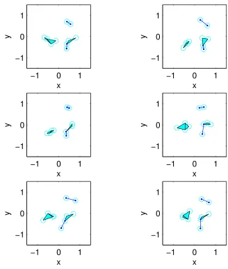
draws. The three models with the highest posterior probabilities are displayed in Table3. The

geo-metric graphs computed from six posterior samples (one every100draws) are shown in Figure11;

note that the computed nerves appear to stabilize after a few hundred iterations while the actual

position of the vertex set continues to vary.

Graph Topology Posterior Probability

[1,4,10][1,8,10][4,5][8,9][2,3,9][6][7] 0.963 [1,4,10][1,8,10][4,5][8,9][2,3,9][6][5,7] 0.021 [1,4,10][1,8][4,5][8,9][2,3,9][6][7] 0.010

Table 3: The three models with highest estimated posterior probability. The true model is shown in bold (see Figure10). Hereθ= 4.

4.2.2 Gaussian graphical model

We use our procedure to perform model selection for the Gaussian graphical model X ∼

No(0,ΣG), where G encodes the zeros in Σ−1. We adopt a Hyper Inverse Wishart (HIW) prior

distribution forΣ| G. The marginal likelihood (in the parametrization ofAtay-Kayis and Massam,

2005, Eqn (12)) is given by

M(V) = (2π)−pN/2 IG(V)(δ+N, D+X

T_X)

IG(V)(δ, D)

, (4.2)

where

IG(δ, D) =

Z

M+_(G)

|Σ|(δ−2)/2e−12<Σ,D>dΣ

denotes the HIW normalizing constant. This quantity is available in closed form for weakly

decom-posable graphsG(V), but for our unrestricted graphs (4.2) must be approximated via simulation.

For our low-dimensional examples the method of (Atay-Kayis and Massam, 2005) suffices; for

larger numbers of variables we recommend that of (Carvalho et al., 2007). We set δ = 3 and

−1 0 1 −1 0 1 x y

−1 0 1

−1 0 1

x

y

−1 0 1

−1 0 1

x

y

−1 0 1

−1 0 1

x

y

−1 0 1

−1 0 1

x

y

−1 0 1

−1 0 1

x

y

−1 0 1

−1 0 1

x

y

−1 0 1

−1 0 1

x

y

−1 0 1

−1 0 1

x

y

Figure 11: Geometric graphs corresponding to snapshots of posterior samples (one every 100 iterations) from model of (4.1a). For this example graphs are constructed to be decomposable and the clique marginals are specified as Clayton copulas.

We sampled300observations from a Multivariate Normal with mean zero and precision matrix

          

18.18 −6.55 0 2.26 −6.27 0

−6.55 14.21 0 −4.90 0 0

0 0 10.47 0 0 −3.65

2.26 −4.90 0 10.69 0 0

−6.27 0 0 0 27.26 0

0 0 −3.65 0 0 7.41

X 3

X 1 X

6

X 5

X 2

X 4

Figure 12: Graph encoding the Markov structure of the model given by precision matrix (4.3).

whose conditional independence structure is given by the graph in Figure 12. We fit the model described in Section 3 using a uniform prior for each Vi ∈ B2 and r = 0.25. We employed

hybrid random walk proposals in which we move all five vertices {Vi} independently according

to the diffusion-inspired random walk described in Section3.2with probability0.85; replace one

uniformly selected vertexVi with a uniform draw fromUn(B2)with probability0.05; and replace

all five vertices with independent unoform draws fromUn(_B2)with probability0.10. We sampled

1 000observations from the posterior after a burn in of750 000. Results are summarized in Table4

Graph Topology Posterior Probability

[1,2,4][1,5][3,6] 0.152 [1,5][2,3,4][2,3,6] 0.072 [1,2,3,4,6][1,5] 0.069 [1,4][2,4][2,3,6] 0.055 [1,2,4][2,3,4][1,5][3,6] 0.052

Table 4: The five models with highest estimated posterior probability. The true model is shown in bold.

4.2.3 Factorization Based on Nerves

While Gaussian joint distributions are determined entirely by the bivariate marginals, and so

possible for other distributions. The familiar example of the joint distribution of three Bernoulli

variablesX1,X2,X3 each with mean1/2, withX1andX2independent butX3 = (X1−X2)2(so

that{Xi}are onlypairwiseindependent) has only the complete set{1,2,3}in its factorization.

Consider now a model with the graphical structure illustrated in Figure13whose density

func-tion, if it is continuous and strictly positive ((seeLauritzen,1996, Prop.3.1)), admits the

complete-set factorization:

f(x| G, θ) =cGφ(x1, x2)φ(x1, x6)φ(x2, x6)·φ(x3, x4, x5). (4.4a)

For illustration we will take eachφ(·)to be a Clayton copula density (see (4.1b)). For simplicity

we specify the same valueθ = 4for each association parameter, sof(x | G, θ)is given by (4.4a)

with

φ(x, y) = 5 (x−4+y−4−1)−9/4 (x y)−5 (4.4b)

φ(x, y, z) = 30(x−4+y−4+z−4 −2)−13/4(x y z)−5. (4.4c)

In earlier examples we associated graphical structures (i.e., edge sets) with 1-skeletons of

nerves. We now associatehypergraphical structures (i.e., abstract simplicial complexes that may

include higher-order simplexes) with the entire nerves, with maximal simplices associated with

complete-set factors. For example: the Alpha complex computed from the vertex set displayed in

Table 5 with r = 0.40has {3,4,5}{1,2}{1,6}{2,6} as its maximal simplices (Figure 14). By

V

2

V

1 V₆

V

3

V

5

V

4

−1 −0.5 0 0.5 −0.5

0 0.5 1

x

y

V

2

V

1

V

6

V

3

V

4

V

5

Figure 14: Alpha complex corresponding to the vertex set in Table5andr=√0.075.

Coordinate V1 V2 V3 V4 V5 V6

x −0.0936 −0.4817 0.0019 0.0930 0.2605 −0.5028

y 0.6340 0.7876 0.0055 0.0351 −0.0702 0.2839

Table 5: Vertex set used for generating a factorization based on nerves.

associating a Clayton copula to each of these hyperedges we recover the model shown in (4.4).

We use the same prior and proposal distributions constructed in Section3.2from point

distribu-tions in_Rd; what has changed is the way the nerve is being used: as a hypergraph whose maximal hyperedges represent factors. One complicating factor is the need to evaluate the normalizing

fac-tor cG for each graph G we encounter during the simulation; unavailable in closed form, we use

Monte Carlo importance sampling to evaluate cG for each new graph, and store the result to be

reused whenGrecurs.

We anticipate that uniform draws Vi

iid

∼ Un(_B2)will give high probability to clusters of three or more points within a ball of radiusr, favoring higher-dimensional features (triangles and

phe-nomenon, we compare results for uniform draws with those from a repulsive process under which

clusters of three or more points are unlikely to lie within a ball of radiusr, hence favoring

hyper-graphs with only edges.

We began by sampling650observations from model (4.4) withA =Alpha andr = 0.40, with

independent uniform prior distributions for the verticesVi

iid

∼Un(_B2)on the unit ball in the plane. The Metropolis/Hastings proposals for the vertex set are given by a mixture scheme:

• A random walk for each Vi as described in Section 3.2, with step size η = 0.020. This

proposal is picked with probability0.94

• An integer1≤k ≤6is chosen uniformly and, givenk, a subset of sizekfrom{1,2,3,4,5,6}

is sampled uniformly; the vertices corresponding to those indices are replaced with random

independent draws from Un(_B2). This proposal is picked with probability 0.06, 0.01 for eachk.

Forθwe used the same standard exponential prior distribution and reflecting uniform random walk

proposals described in Example4.2.1.

Using5 000posterior samples after a burn-in period of95 000iterations, the models with

high-est posterior probability are summarized in Table6.

To penalize higher-order simplexes we used a Strauss repulsive process (Strauss,1975)

condi-tioned to haveppoints in_Bdas prior distribution for the vertex set, with Lebesgue density

g(v)∝γ#{(i,j):dist(vi,vj)<2R}

for some0< γ≤1, penalizing each pair of points closer than2R. Simulation results for this prior

(withR = 0.7randγ = 0.75) are summarized in Table7. The posterior mode is far more distinct

for this prior than for the uniform prior shown in Table6.

Maximal Simplices Posterior Probability

{3,4,5}{1,2}{2,6}{1,6} 0.609

{1,2,6}{3,4}{4,5}{3,5} 0.161

{3,5}{1,6}{3,4}{1,2}{2,6} 0.137

Maximal Simplices Posterior Probability

{3,4,5}{1,2}{2,6}{1,6} 0.824

{1,2,6}{3,4,5} 0.111

{1,2,6}{3,4}{3,5}{4,5} 0.002

Table 7: Highest posterior factorizations with Strauss prior (true model is shown in bold).

In a further experiment withγ = 0.35, the posterior was concentrated on factorizations without

any triads.

4.2.4 GOutside the Space Generated byA

In the simulation studies of Sections 4.2.1–4.2.3the class of setsAused to compute the nerve

was known. In this example we investigate the behavior of our methodology when the class of

convex sets used to fit the model differs from that used to generate the true graph. We consider

three possibilities: A =Alpha in_R2,A =Alpha in_R3 andA = Cech inˇ _R2. We performed two experiments: one when the graph is feasible for each the three classes, and another example where the graph could be generated by only two of the classes.

First consider a model with junction tree factorization:

fθ(x) =

ψθ(x1, x3)ψθ(x2, x3, x4)ψθ(x5)

ψθ(x3)

, (4.5)

whose conditional independence structure given by the graph of Figure 15. Again, the clique

marginals are specified as a Clayton copula with θ = 4. We simulated 300 samples from this

distribution.

We fitted the model with each of the three classes of convex sets using the Metropolis Hastings

algorithm of Section 3.2 with random walk proposals on _Bd (where d = 2 or 3, depending on

A). Algorithm 1was used to enforce decomposability, usingr = 0.40andη = 0.020. The same exponential prior and uniform reflecting random-walk proposals for θ were used as in Example

4.2.1. Results of1 000samples after a burn-in period of50 000draws are summarized in Table8.

Not surprisingly, the posterior mode coincided with the true model in all three cases.

The second model we considered has junction tree factorization:

fθ(x) =

ψθ(x1, x2, x4)ψθ(x1, x3, x4)ψθ(x1, x4, x5)

(ψθ(x1, x4))2

−1.5 −1 −0.5 0 0.5 1 1.5 −1.5

−1 −0.5 0 0.5 1 1.5

x

y

V

1

V

5

V

2

V

3

V

4

Figure 15: Graph encoding the Markov structure of the model given in (4.5).

Nerve HPP Models Posterior

Alpha in_R2 [1,3][2,3,4][5] 0.964 [1,3][2,3,4][1,5] 0.012 [1,3,4][2,3,4][5] 0.012

Alpha inR3 [1,3][2,3,4][5] 0.982

[1,3][2,3][3,4][5] 0.011 [1][2,3,4][5] 0.003

ˇ

Cech in_R2 _{[1,3][2,3,4][5] 0.595}

[1,2,3,4][5] 0.179 [1,2,3,4,5] 0.168

Table 8: Models with highest posterior probability. The table is divided according to the class of convex sets used when fitting the model. The true model is shown in bold.

The corresponding graph cannot be obtained from an Alpha complex in _R2, but it is feasible for an Alpha complex in _R3 (Figure16) or a ˇCech complex in _R2. Using the same Clayton clique marginals before, we sampled 300 observations from this distribution and fitted the model using

the three classes of convex sets. Results from 1 000 samples after a burn-in period of 75 000

−1 −0.5

0 0.5

1

−1 −0.5 0

0.5 1 −1

−0.5 0 0.5 1

V

2

V

3

V

5

V

4

V

1

Figure 16: Graph encoding the Markov structure of the model given in (4.6).

Nerve HPP Models Posterior

Alpha in_R2 [1,2][1,3,4][1,4,5] 0.214 [1,2,4][1,3,4][1,3,5] 0.115 [1,2,4][1,3,4][3,4,5] 0.112 Alpha inR3 [1,2,4][1,3,4][1,4,5] 0.976

[1,2,3,4][1,4,5] 0.016

[1,2,4][1,3][1,4,5] 0.009 ˇ

Cech in_R2 [1,2,4][1,3,4][1,4,5] 0.758 [1,2,4][1,3,4][1,3,5] 0.177 [1,2,4][1,3,4][4,5] 0.148

Table 9: Models with highest posterior probability, for each class of convex sets. The true model (shown in bold) is unattainable for Alpha complexes in_R2.

mode (unlike the previous example, or Sections4.2.1and4.2.3). The posterior mode for the ˇCech

complex in_R2 and the Alpha complex in_R3 both match the true model.

4.3

Comparative performance analysis with state-of-the-art

We compared the performance of our method to Feature Inclusion Stochastic Search (FINCS),

proposed byScott and Carvalho(2008), and the adaptive LASSO as described in the paper byFan et al.(2009). The criterium for the comparison was given by estimating the counts of specific

the absolute counts for the following subgraphs: triangles, 4-cycles, 5-cycles, 3-stars, 4-stars, and

5-stars, for the true graph and for the estimated network by our method and its competitors, then

we computed the absolute difference between the counts for the true and estimated graph and then

divided by the count for the true graph. We denote by an∗the counts of induced subgraphs; this measures the performance of the methods under decomposability. We generated the set of true

networks from an Erd¨os-R´enyi random graph model withα= 0.05, so we are in a regime that can

be called sparse.

To fit our method, we assumed an uniform distribution on the unit ball in R3 for the vertex

set and for the radius of each vertex an Ex(0.1) as priors. For the positions of the vertices we used the same proposals as in Examples 4.2.1 - 4.2.4. For each radius we implemented a

mix-ture of random walks reflecting at 0as proposal. We used the nerve corresponding to the Cech

complex. We set up FINCS with a probability of 0.1 for resampling moves and a probability

of 0.1 for global moves. For the adaptive LASSO we set up γ = 0.5 and Ω was initialized as

the inverse of the sampled covariance matrix. Subgraphs were counted using the igraph

com-mand graph.subisomorphic.lad. When computing the normalized error, we adopted the convention

0/0 = 0. For the induced subgraphs, we only compute the error of the Bayesian procedure and

Lasso over the set of non-decomposable graphs. For the simulation displayed in Table10all100

graphs were non-decomposable.

Results are summarized in Table10. Our method incurred into less errors on average compared

to our competitors for almost all subgraphs. The exception was the5−star. We also observed that

FINCS outperformed the LASSO for almost all regimes, with exception of the5−star.

We performed another simulation, now assuming an exponential random graph model for the

true graph. The simulation of the true graphs was implemented using the R package statnet. We

Subgraph Bayes FINCS Lasso

triangles 0.083±0.07 0.125±0.17 0.208±0.12

4- cycles 0.062±0.10 0.123±0.16 0.166±0.10

5- cycles 0.086±0.07 0.112±0.14 0.124±0.08

3- stars 0.103±0.08 0.139±0.12 0.211±0.08

4- stars 0.087±0.08 0.096±0.16 0.115±0.11

5- stars 0.201±0.10 0.183±0.14 0.174±0.06

4- cycles∗ 0.146±0.12 0.930±0.07 0.229±0.12

5- cycles∗ 0.128±0.13 1±0 0.174±0.08

Figure 17: Here we compare the true model, which was sampled from the ERGM used in Table

11, and the fitted model, using our method (again, as in Table11). The edges that were added by our method (with respect to the true graph) are highlighted in red. The edges that were deleted by our method are highlighted in green.

used the formula edges+triangles+kstar(3), with coef=c(-3.2,0.95,0.005); this specification

encour-ages the presence of triangles and 3-stars. These choices produce graphs with twice the 3-stars and

3 times more triangles than an Erd¨os-R´enyi withα = 0.05, while having approximately the same

density. The objective of this experiment is to investigate the behavior of our method when the true graph has more structure than the typical realization of an Erd¨os-R´enyi model. Results are

summarized in Table 11; they are similar to what was observed in the previous experiment. We

observed an improvement regarding the counts of triangles, this is not surprising since geometric

random graphs tend to have more triangles than realizations from an Erd¨os-R´enyi model. In Figure

17we compare the true model (as generated from the ERGM just described) and the fitted model

for a single realization. In this regime, graphs tend to be non-decomposable. We estimated the

proportion of decomposable graphs from a sample of 1,000 networks sampled from the ERGM

used to obtain the simulation in Table 11, and obtained 0.302 as the result. For the simulation

Subgraph Bayes FINCS Lasso triangles 0.071±0.04 0.134±0.14 0.217±0.09

4- cycles 0.067±0.06 0.121±0.12 0.154±0.04

5- cycles 0.075±0.09 0.118±0.11 0.131±0.13

3- stars 0.092±0.07 0.144±0.14 0.236±0.12

4- stars 0.086±0.09 0.115±0.15 0.117±0.10

5- stars 0.214±0.09 0.122±0.13 0.121±0.06

4- cycles∗ 0.152±0.12 0.720±0.07 0.214±0.10

5- cycles∗ 0.133±0.10 0.720±0.13 0.163±0.08

Table 11: Estimated normalized errors for counts of specific subgraphs for our method, FINCS and adaptive LASSO. The true graphs were sampled from an ERGM that encouraged the presence of triangles and 3-stars.

4.3.1 Scalability

Here we discuss scalability of the proposed method and of the competing methods (Fan et al.

(2009),Scott and Carvalho(2008)) to better appreciate the cost incurred in producing the errors in

Tables10and11. Since the implementation of the proposed and competing methods available to

us are in different programming languages, which influence greatly the actual runtime, we outline

such a discussion in theory, in terms of key quantities that influence scalability, including number

of nodesn, number of edgesm, and number of cliquesk. We also distinguish two tasks: the task of estimating the parameter of a model-based representation of a (hyper)graph, and the task of

generatingb(hyper)graphs from an estimated model-based representation.

Regarding the task of estimating parameters from an observed (hyper)graph, the proposed

meth-ods requires estimating parameters{V}, r, and the estimation complexity scales asO(S(n) +k3_),

whereS(n)denotes the complexity of matrix multiplication.1 The method byScott and Carvalho

(2008) requires estimating parametersG, and the estimation complexity scales as O(S(n) + k).

The lasso requires estimating parametersΣ−1_{, and the estimation complexity scales asO(n}3_).

Regarding the task of generating b (hyper)graphs from an estimated model-based

representa-tion, the proposed methods scales as O(bn2_{). This is because the complexity of computing the}

2-skeleton of the Cech complex scales asO(n2_{). Alternative representations lead to different}

scal-ing: computing the Delaunay triangulation scales as O(nlogn), and computing the the Alpha

complex scales as O(n2_{). The method by Scott and Carvalho (2008) scales as O(bnm), where}

typicallymis much larger thann. For the lasso, this statement does not apply.

1_{The parameterkin this case is actually the number of prime components, but this quantity is typically in the same}

To illustrate how our method scales up with respect to the number of variables, we ran the

ex-periment summarized in Table12. We obtained the graphs from the nerves of ˇCech complexes and

employed the method proposed by (Atay-Kayis and Massam, 2005) to compute the normalizing

constants of non-decomposable graphs. The MCMC was performed on a 2.5GHz desk computer with 4GB of RAM. Our method was implemented using Matlab (MathWorks).

N Variables Burn-in N Iterations Time

4 50,000 10,000 7m

40 50,000 10,000 2h11m

400 50,000 10,000 3d2h17m

Table 12: This experiment illustrates how our method scales up with respect to the number of variables.

4.4

Real data analysis

4.4.1 Fisher’s Iris data

We applied our method to Fisher’s Iris data set. Variables include: sepal length (1), sepal width

(2), petal length (3), and petal width (4). The objective is to find the conditional independence

structure given a family of distributions for the likelihood (e.g. Gaussian, Clayton copula). A

summary of the distribution of this data set is given in Table13

We first describe the specification we used for the random geometric graph, then we will make

our choices for the Hyper-Markov law and the likelihood explicit. For the RGG we assumed an

uniform distribution of the vertices on the unit ball in _R3 _{and for the radius of each vertex an}

Ex(0.1), distribution was assumed. For the positions of the vertices we used the same proposals as in Examples4.2.1-4.2.4. For each radius we used a mixture of random walks reflecting at0as

proposal. For the likelihood function and Hyper-Markov law we used the following specifications:

Variable SL SW PL PW

Sepal length 0.4043

Sepal width 0.0938 0.1040

Petal length 0.3033 0.0714 0.3046

Petal width 0.0491 0.0476 0.0488 0.0754

A multivariate normal distribution for the likelihood with an HIW as Hyper-Markov law.

For our choice for the likelihood and Hyper-Markov law, we adopted the same values for the

hyperparameters as (Roverato, 2002) did, this is, the prior for the precision matrix centered at I

and δ = 3. We used the method proposed by (Atay-Kayis and Massam, 2005) to deal with the

normalizing constants of non-decomposable graphs. We ran the MCMC with300 000iterations as

burn-in and kept the last10 000for analysis.

Results for the first choice are summarized in Table 14. Here we display the9 models with

highest posterior probability. All the posterior probability was concentrated in this models. Our

posterior mode coincides with the one reported by (Roverato, 2002), but we obtained different

results for the rest of the models. We attribute this difference to the fact that we used different

priors for graph space; ours being non-uniform.

We conducted another simulation, where we assessed the robustness of the inference for the

Maximal Simplices Posterior Probability

{1,2}{1,3}{2,4}{3,4} 0.3465

{2}{1,3}{3,4} 0.2835

{1,3}{2,3}{4} 0.1999

{1,2}{1,3}{4} 0.1540

{1,2}{1,4}{2} 0.0116

{1,4}{2}{3,4} 0.0026

{1,2}{1,3}{3,4} 0.0016

{1,3}{2,3}{3,4} 0.0002

{1,4}{1,3}{2,3}{3,4} 0.0001

Table 14: Highest posterior factorizations with uniform prior and Gaussian distribution for Fisher’s Iris data set.

Maximal Simplices Frequency as posterior mode

{1,2}{1,3}{2,4}{3,4} 0.68

{1,3}{2,3}{4} 0.16

{1,2}{2,3}{2,4} 0.08

{1,4}{2,4}{3,4} 0.04

{1,4}{1,3}{2} 0.04