Policy instruments to control Amazon fires:a simulation approach

1 Policy instruments to control Amazon fires: a simulation approach

Abstract

Agricultural fires are a double-edged sword that allow for cost-efficient land management in the tropics but also cause accidental fires and emissions of carbon and pollutants. To control fires in Amazon, it is currently unclear whether policy-makers should prioritize command-and-control or incentive-based instruments such as REDD+. Aiming to generate knowledge about the relative merits of the two policy approaches, this paper presents a spatially-explicit agent-based model that simulates the causal effects of four policy instruments on intended and unintended fires. All instruments proved effective in overturning the predominance of highly profitable but risky fire-use and decreasing accidental fires, but none were free from imperfections. The performance of command-and-control proved highly sensitive to the spatial and social reach of enforcement. Side-effects of incentive-based instruments included a disproportionate increase in controlled fires and a reduced acceptance of conservation subsidies, caused by the prohibition of reckless fires, and also indirect deforestation. The instruments that were most effective in reducing deforestation were not the most effective in reducing fires and vice-versa, which suggests that the two goals cannot be achieved with a single policy intervention.

2 1 Introduction

Fire is one of the major socio-environmental challenges facing the humid tropics, including the Amazon Basin. On the one hand, fire is an efficient tool to prepare, weed and fertilize land, and it provides profit and subsistence to a wide range of farmers from smallholders to large cattle ranchers. On the other, it is a source of escaped fires and atmospheric pollutants, a potential cause of soil degradation and a threat to rainforests, biodiversity and farmers' assets and health (Nepstad et al. 2001 and 2007, Mendonça et al., 2004, Chen et al., 2011, Carmenta et al., 2013). Furthermore, the likelihood of disastrous wildfires this century is increased by predicted climate and vegetation changes linked to a higher frequency of extreme droughts, (Malhi et al., 2009, Chen et al. 2011, Coe et al, 2013, Davidson et al, 2012). For example, in 1998 fires in the Brazilian Amazonian state of Roraima affected over 5 million hectares of forest (Cochrane, 2009, p.17), while 2015 was the hottest year in the amazon over the last century (Jiménez-Muñoz et al., 2016).

Preventing an increase in the prevalence of fires in the Amazon and elsewhere requires policies that internalize externalities (Malhi et al., 2009, Sorrensen, 2009, Carmenta et al, 2013). In Brazil, one of the federal government’s main responses to the fire problem is the controlled burn law, which replicates the ban-surveillance-sanction approach that proved highly successful for deforestation. Yet, to-date, there is no assessment of the impact of this policy on fires. Interventions are also occurring at local scales, including incentive-based initiatives of payment for avoided deforestation and avoided forest degradation (REDD+), as well as municipal actions supporting mechanized land preparation substituting for slash-and-burn (Simões and Schmitz, 2000, Börner et al., 2007 and 2013, SEMA-AC, 2011).

The evaluation of impacts and limitations of command-and-control and incentive-based approaches to policy requires reliable empirical evidence. However, empirical work cannot provide definite answers without being guided by refutable hypotheses. This paper seeks to contribute with such hypotheses by developing an analytical device that represents the Amazon fire system both in the absence and presence of intervention. This is achievable with an agent-based, spatially-explicit simulation model. Policies, such as agricultural subsidies or payment ecosystem services (PES), aim to influence decisions with supra-individual consequences made by heterogeneous individuals. Policy interventions inevitably trigger a chain of connected processes whose net impact on the key state variables is not easy to intuit from pure reasoning without the support of an analytical tool. It is in this particular sense that a simulation model is useful (Zhao et al, 2012).

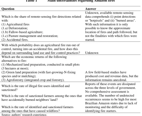
3 Two are the main reasons for adopting agent-based modelling. First, its bottom-up approach enables multiple possibilities of individual and collective reactions to policy, including those that would prevent desired outcomes from being achieved or would favor undesired results. Second, it generates results with a level of heterogeneity/variability which reasonably resembles the data available for policy evaluation. However, regarding this second reason, a clarification is needed. Part of the richness of the results is very hard to reduce to refutable hypotheses that may guide policy evaluation. As producing such hypotheses is one of our main goals, we opted for a causal inference approach to simulation analysis (Marshall and Galea, 2014). This means focussing on comparing policy outcome variables in baseline and policy scenarios, rather than exposing the plethora of patterns the variables describe across time and space. The model presented in this paper is a tool to build knowledge on the potential results of policy options to reduce Amazon fires. Due to the scarcity of knowledge on this topic, we opt to focus the modelling effort on detailing a few key components of the Amazon fire system, mainly farmer behavior and policy instruments, and incorporate other aspects in a rather stylized way. This approach strives to maximize the usefulness of the exercise for empirical work, because scant existing evidence (table 1) does not allow for testing of the intricate hypotheses that would be yielded by a more comprehensive model. There is a further methodological reason for adopting a simple (or stylized) model. A clear trade-off exists between realism (the number and detail of real-world natural and social processes represented) and identification of causal effects (the confidence that observed variations in outcome variables are strictly due to variations in policy). Simulation models are different from models with analytic (pen-and-paper) solutions in that they do not necessarily yield identification. Non-linearity and stochasticity, coupled with endogeneization of most variables, makes it hard to track the causes of the observed behavior of the main variables (Marshall and Galea, 2014). This difficulty grows with realism (El-Sayed et al., 2012, Cederman and Giradin, 2007, Townsley and Birks, 2008). We opt first of all for causal effect identification and pay the cost of reduced realism by greatly simplifying the Amazon fire system. The main benefits are the clarity and the empirical refutability of the hypotheses about the impacts of policy that can be derived from the results.

The policy background is synthesized in the next section and the model is presented in section three. The results are analyzed and interpreted in section four, followed by a brief conclusion.

Table 1 [here] 2 Fire policy in Brazil

2.1 Brief overview

4 against agricultural fires that have a high probability of turning into uncontrolled fires and causing major damage (Brasil, 1998, Steil, 2009). However, in practice, permit granting is marginal (Toniolo, 2008, p.193-194, Carmenta et al., 2013, Cammelli, 2014, p. 13, Costa, 2004, p. 184), enforcement is rare (IBAMA-PA, 2015) and recent fieldwork1 indicated that few state and local governments execute these functions. The main barriers for the farmers are the transaction costs of obtaining the documents demanded by permit requisition, especially the proof of land ownership, travelling often long distances from farms to environmental offices in urban areas (Carmenta et al., 2013, Cammelli, 2014, p.48).

Second, subsidies have been used to reduce fire and offer different routes for promoting the technological transition of smallholders to fire-free agriculture; mechanization and agroforestry. These include subsidies for mechanized land preparation offered by some municipal governments, generally together with extra financial support for agricultural inputs (Börner et al, 2007, Emater, 2015b, Simões and Schmitz, 2000). Alternatively, pilot projects are used to stimulate agroforestry systems, which combine trees, crops and animals in the same plot without resort to fire or inputs. The agroforestry pathway tends to be funded by NGOs and public institutions, and is advocated as “greener” and more sustainable than mechanization (Serra, 2005, Arco-verde, 2008, MMA, 2009). However, progress on these fronts tends to be inhibited by constraints facing the targeted farmers, including lack of access to capital and credit, labor, inputs and rural extension services. Two of these constraints are critical for the shift to agroforestry. First, labor, since agroforestry requires a higher working effort, at least initially (Arco-verde, 2008, p.93). Second, credit, as public and private banks still lack a standardized methodology to estimate the profitability of agroforestry systems with sufficient certainty (Emater, 2015a, Kato, 2015).

Third, PES represent incentive-based instruments to reduce fires. An exemplar scheme was the Proambiente program, based on payment for avoided deforestation and multiple related ecosystem services including reduced wildfire risk. This program provided payment and technical support between 2004 and 2008 to enable four thousand smallholder households across the nine states of Legal Amazon to adopt fire-free practices (Hall, 2008, Neto, 2008, p.20, Wunder et al., 2009). Another example is the Bolsa Floresta program, which transfers cash to forest-dependent communities conditional on forest conservation and avoided carbon emissions. In some cases, transfers are conditional also on the control and reduction of fire use (Börner et al., 2013). However, at present PES programs in the Amazon are restricted to a few projects with only localized impacts. This contrasts with the growing number of papers arguing that incentive-based instruments are the best way to conserve tropical forests and control fires (e.g. through payments for reduced emissions from deforestation and degradation (REDD+; Barlow et al, 2012; Aragão and Shimabukuro, 2010).

2.2 Simulated policy instruments

5 The model simulates the impacts of simplified representations of three of the classes of policy instruments, namely the controlled burn law (i.e. command-and-control), a subsidy scheme for transition to fire-free agriculture through mechanization and PES schemes (technical details are found in appendices A and B).

A command-and-control (C&C) instrument was simulated by assuming that the environmental authority bans and sanctions only “reckless fires”, i.e., agricultural fires with high probability of running out of control and turning into accidental fires. Accounting for the low spatial resolution (1 km2 cells) of remote-sensing fire detections that fire monitoring by the Brazilian government is based on (Vasconcelos et al., 2013, INPE, 2015, PREVFOGO, 2015), the modelled landscape used in our simulations was divided into “monitoring zones” of 1 km2. Monitoring can only effectively identify fire-users where a zone intersects a single farm (as opposed to parts of multiple farms occupying the same zone). Reckless fires detected in single-farm zones (herein, enforcement-effective zones) generate a fine of fixed value per hectare which is applied to the owner. It is assumed that farmers know perfectly in which zones enforcement is effective.

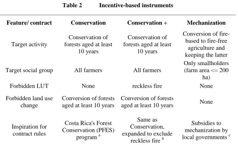
Second, subsidy schemes, also referred as “incentive-based instruments”, are represented as voluntary contracts of three modalities. Each modality targets the promotion of a specific mix of land use and technology (LUT) that can be developed in the parcels in which landscape is subdivided. This includes not only PES schemes but also the subsidy to fire-free agriculture (table 2). The agroforestry route is not modelled for consisting in complex mixes of crops, trees and cattle which take highly heterogeneous and mostly experimental forms in the literature (Serra, 2005, Arco-verde, 2008, MMA, 2009).

The total annual subsidy received by a farmer is the product of the number of parcels with the target activity by a fixed per-hectare basis subsidy. All contracts have a five-year lifetime and are renewable indefinitely. Payment of subsidies occurs every year and is conditional on the compliance of contractual norms (table 2). If any norm is violated, the farmer must return all annual payments received since the start of the current contract. This stiff penalty of early contract termination is employed to assure time-consistency (Gulati and Vercammen, 2006).

Table 2 [here] 3 The model

3.1 Presentation strategy

6 i.e. the translation of concepts into an implementable procedure of algorithms and equations, is left to appendices and supplementary material. This simplified presentation strategy adheres to the fundamental ODD+D principle of gradually introducing the reader to model details.

3.2 Description of the model

Here we present a brief summary of the detailed description found in appendices A and B. 3.2.1 Purpose

The model is a tool to build knowledge on the impacts and limitations of command-and-control and incentive-based policy instruments designed to command-and-control agricultural and accidental fires in the Brazilian Amazon.

3.2.2 Entities, state variables and scales

Four kinds of entities populate the model: farmers (decision-makers), parcels (spatial units), government and nature.

There are four combinations of land use and technology (LUTs, herein) a land parcel can be allocated with. Three of them are agricultural land uses, namely, agriculture based on “controlled fires” (hereafter “controlled fires”), agriculture based on “reckless fires” and “fire-free agriculture” (herein “fire-free”). Reckless fires are conducted without any measure of control such as firebreak construction, burning against the wind or the avoidance of dry periods of the year. Controlled fires take place with the proper control measures, and fire-free agriculture without the use of fire. The remaining land use is forest. Parcels with agricultural LUTs can be converted to forest. In the year when the conversion is made, the parcel’s forest age is set to zero. Therefore, the amount of above-ground forest biomass accumulated in the parcel becomes positive only one year after conversion, which incorporates the delayed regeneration observed in practice (Neeff and Santos, 2005).

Farmers decide the LUT portfolio that prevails on a particular set of parcels (farm). They are characterized by their (i) farm, i.e., the set of parcels controlled, (ii) wealth, (iii) accumulated local data on LUTs and accidental fires, (iv) point estimates for parameters behind the probability of accidental fires which is herein referred to as “risk” (see 3.2.3 below) and (v) status regarding subsidy contracts.

7 Nature is an observer or “higher-level controller” (Grimm et al, 2010) that decides which parcels are affected by accidental fires at each time step. It is the only entity that knows the true risk parameters and also the values of the random component of parcels’ risk (see “define-burned-parcels in next subsection an on appendix B). The government is also an observer. It sanctions reckless fires in the C&C simulations and also offers and monitors voluntary contracts in the incentive-based simulations.

Regarding scale, one time step represents one year, simulations were run for 40 years, one grid cell represents 1 hectare and the model landscape comprises 100 x 100 hectares, i.e., 100 km2.

3.2.3 Process overview and scheduling

There are three classes of simulations. Baseline simulations, in which no policy instrument is active, simulations in which only the C&C instrument is active and simulations in which only incentive-based instruments are active. The last class subdivides into three, each comprising a particular kind of subsidy contract (section 2.2 above).

In baseline and C&C simulations, nine modules are processed in the following order: calculate-profit, implement-LUT-portfolio, LUC-cost-account, define-burned-parcels, sanction-rule-breakers, calculate-actual-profit, update-risk-parameters, store-LUT-portfolio-in-memory, and update-forest-age-after-burn. In incentive-based simulations, the same procedures are processed together with two extra procedures: (i) subsidy-payment-account which is deployed right after "implement-LUT-portfolio" and; (ii) update-contract-duration, deployed right after "LUC-cost-account".

The main features of the modules are described below

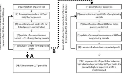
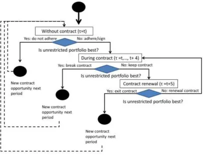
Calculate-profit (figure 1) defines the LUT portfolio to be implemented in each time step using whole-farm expected profit optimization. Instead of seeking the best LUT portfolio globally, the algorithm identifies the best LUTs for each parcel locally by taking as given the best LUTs of neighboring parcels (queen criteria of contiguity was adopted). In other words, it makes assumptions about neighboring best LUTs. Since this profit-calculation is done sequentially for all parcels, the best LUTs of some neighboring parcels may not yet be defined (i.e., remain unknown) at the stage where the best LUT of a given parcel is to be defined. To mitigate against this, identification of best LUTs for all parcels is iterated until it stops yielding an increase in whole-farm expected profit. Due to limited wealth and the costs of changing between land-uses, farmers prioritize parcels with the highest degree of physical suitability. In incentive-based simulations, "calculate-profit" is subdivided into two sub-procedures (route B of figure 1); one that imposes compliance to contract norms (“restricted identification”) and one that does not (“unrestricted identification”). Both these sub-procedures are executed at every step, generating the information that forms the basis of farmers’ decisions on voluntary contracts.

8 function of two classes of factors. First, variables indicating the parcel's own and neighboring parcels' LUTs. Second, fixed ‘risk parameters’ that measure the intensity with which LUTs influence risk. Whether an accidental fire occurs in a parcel is determined by the probability level (risk) and by a standard Gaussian disturbance representing non-observables behind risk. Further details, including the functional form linking LUTs with risk, are found on appendix B, section B.8 (with the complete description of the functional form detailed in appendix C. It is helpful to clarify that fire spread is not modelled. Accidental fire is conceived, for simplicity, as a point event, completely restricted to the parcel where it takes place. Parcels accidentally burned generate zero actual profit. For simplicity, it assumed that the above-ground biomass of forested parcels is fully eliminated by accidental fires (defined as “functional deforestation” by Barlow et al., 2012).

Update-risk-parameters is executed by farmers. Such entities are ignorant of true risk parameters but are able to estimate them. For this, they apply a statistical routine to accumulated local data on LUTs and accidental burns. Only their own parcels and parcels within 100 m of farm boundaries are observed by the farmers. At each time step, parameters are re-estimated after data update.

Implement-LUT-portfolio assigns best LUTs for parcels processed by calculate-profit and previous LUTs for remaining parcels. This is preceded, in incentive-based simulations, by the choice between the LUT portfolio designed to comply with contract norms and the unrestricted LUT portfolio. The choice criterion is to pick the option with the highest whole-farm expected profit.

Update-contract-duration is only part of incentive-based simulations. It defines contract status in the basis of (i) LUT portfolio choice made in the previous procedure and (ii) current contract duration. The possible statuses or actions towards contracts are sign or don’t sign, keep or break, and renewal or exit

3.2.4 Design concepts

Theoretical and empirical background: profit and risk spillovers

9 al, 2003, Stouffer and Bierregaard, 1995). It therefore seems valid to assume that availability of forest resources) in a forested unit of land increase with the amount of forest in the vicinity. Third, surrounding forests mitigate risk (Brando et al., 2013). The magnitudes in which forest services are provided, and the profit made out of forest products, are assumed to be positively correlated with above-ground biomass of the forest accumulated in the source parcel.

It is assumed that risk increases with the agglomeration of fire-based agriculture. Since accidental fires impose economic losses to farmers, this assumption creates a force that favors dispersion of fire-based agriculture (table 3; better detailed in “expected profit function subsection” below).

Table 3 [here] Empirical data

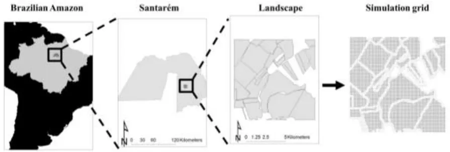
The land property structure, initial location of forest and non-forested parcels and values for physical suitability come from empirical GIS data describing the condition in 2010 of a 10 x 10 km square sub-area of Santarém municipality, in the Brazilian Amazon converted into a 100 x 100 cell digital grid (figure 2, details on SM.1). Physical suitability is measured in terms of slope of terrain, distance to roads and urban centers. Land use change cost was estimated from secondary data (SM.2). Forest-growth follows the empirical above-biomass (logistic) growth function estimated by Neeff and Santos (2005).

10 Figure 2 The modelled landscape in the Brazilian Amazon and the gridded version

used in simulations

Individual Decision Making: statement of the decision problem The problem solved each time step by the i-th farmer is:

Max _{𝜏

𝑘}𝑘=1𝐾𝑖 ∑ 𝑟 𝑒_(𝜂

𝑘, 𝜏𝑘, 𝜏𝑘′, 𝜏𝑘𝑒, 𝛽̂, 𝛾) 𝐾_𝑖

𝑘=1

s. t. ∑ 𝐶(𝜏_𝑘, 𝜏_{𝑘,𝑡−1})

𝐾_𝑖

𝑘=1

≤ 𝑊, 𝛽̂ = f(D)

Where parcels are indicated by k and the following definitions apply: re(.) ≡ expected profit function, ηk ≡ physical suitability, τk ≡ k-th parcel’s LUT, τk’≡ vector with LUTs of neighboring parcels owned by the i-th farmer, 𝜏_𝑘𝑒 _{≡ vector with forecasted LUTs of}

neighboring parcels owned by other farmers, 𝛽̂ ≡ vector with estimated parameters for the accidental fire prediction model (or “risk model”), γ ≡ vector with policy variables including LUT restrictions and magnitudes of subsidies and fines, C(.) ≡ LUT change cost (computed by “LUC-cost-account” procedure), τk,t-1 ≡ previous LUT, W ≡ wealth, f(.) ≡ function representing the estimation of 𝛽̂, D ≡ current data on observed accidental fires (automatically updated; see “update-contract-duration” above).

In a nutshell, farmers choose the LUT portfolio that yields the highest farm-level expected profit, given the norms of prevailing policy (γ), knowledge on the likelihood (risk) of accidental fire occurrence (𝛽̂), forecasts for neighbors LUT choices (𝜏_𝑘𝑒_{), and the constraints}

11 The model reduces to a computational implementation of the problem just described. Results generated are a set of solutions to the problem for all agents at all time steps.

Individual Decision Making: solution of the decision problem

The farmer’s decision problem is solved with the “calculate-profit” procedure (figure 1, section 3.2.3) which seeks to represent Amazonian farmers’ decision-making. Multiple studies attest the influence of capital on land use decisions, here called “wealth”, and of the parcel-scale factors determining physical suitability, being them slope of the terrain and distance to roads and urban centers (Deadman et al., 2004, Sorrensen, 2000 and 2004, Moran et al., 2002, Scatena et al., 1996, McCraken et al. 2002). In particular, the wealth allocation principle of giving priority to parcels whose costly conversion is, due to physical factors, more profitable, is supported by empirical evidence that proximity to roads, urban centers and flat terrain have positive effects on deforestation (Pfaff, 1999, Pfaff et al., 2007).

The procedure is also designed as a bounded rationality shortcut to the search for the best among all possible portfolios, which amount to a number of alternatives whose order of magnitude is of 1018 for a 30-hectare farm, the smallest size considered. Two approaches to land use economics are reconciled by the LUT choice algorithm. The multi-output approach (e.g., Just et al, 1983, Fezzi and Bateman, 2011), for which farmers’ choice is guided by whole-farm profit, and the recent spatially-explicit models (e.g., Irwin and Bockstael, 2001, Parker and Meretsky, 2004), which emphasize heterogeneity and spatial externalities at parcel-level.

Expected profit function

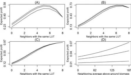
Parcel-level expected profit function is re = ηθ(1-p) – C(.) + S(γ), with η ≡ physical suitability, θ ≡ deterministic profit, p ≡ probability of the parcel to be accidentally burned or simply “risk”, C(.) ≡ LUT change cost, S(γ) ≡ fine (negative value) or subsidy (positive value) assigned by policy. The main forces driving LUT choice in the model, the agglomerative and dispersive forces (table 3), are captured by two components, θ and p. To simplify language, only the product θ(1-p) is hereafter referred as “expected profit function”. The arguments of θ and p are metrics for three classes of variables, (i) own-parcel LUT, (ii) neighboring parcels’ LUTs, (iii) forest biomass either (iii.a) in the parcel (if occupied with forest) or (iii.b) in neighboring parcels. Details on the metrics and how they enter the functional forms of θ and p are provided in appendix C. Agglomerative and dispersive forces captured by θ are indicated with “[θ]” in table 3 and those captures by p with “[p]”. Expected profit functions are shown in figure 3. Farmers optimize an average of these functions weighted by physical suitability. For non-forest LUTs, the horizontal axis measures the degree of agglomeration in terms of neighboring parcels2 with the same LUT as the reference parcel. The higher the average forest biomass in neighboring parcels, the higher the curve. For the case of forest, the agglomeration degree is measured as neighboring parcels’ average above-ground biomass of forest. Higher curves represent higher levels of parcel’s own forest biomass. As the figure shows, expected profit functions are concave as agglomeration has

2

12 decreasing returns for all non-forest LUTs, what is in line with standard assumptions in economics (see, for instance, Mas-Colell et al., 1995, p.133-137, Varian, 1992, section 2.1, Doole and Kingwell, 2015, 2.1). This stems from the positive effect of agglomeration on both deterministic profit and risk.

For the case of forest, agglomeration has opposite effects, positive for deterministic profit and negative for risk, yielding, thus, increasing returns. However, the expected profit of forest is concave in forest age, or equivalently, in own-parcel biomass, what stems from the logistic function driving forest growth (obtained from Neeff and Santos, 2002). Such concavity is attested by the bottom left of figure 3, where there is a decreasing distance in between two subsequent curves. Such is also the case for non-forest land uses. Consequently, the expected profits of all LUTs are concave in neighboring average forest biomass.

Concavity is merely an expression, in the form of expected profit, of the more general idea of agglomerative and dispersive forces, in particular the forces specified in table 3. The optimal agglomeration level is the lowest for reckless fire as such LUT, by definition, has higher probabilities of turning into an accidental fire, for each agglomeration level. Also influent in such respect is a low level of scale economy (table 3). In contrast, fire-free has the highest optimal agglomeration level due to zero reliance on fire, and thus, low exposure to accidental fires and also to a high level of scale economy (table 3). All non-forest LUTs are supported by forest services, what explains the positive effect of surrounding forest biomass in their expected profits. Forest is subjected to returns from agglomeration as the process increases its capacity to generate services that provide self-support (table 3). The low expected profit forest is assumed to generate accounts for the still relevant deforestation level (~5,000km2/year, Godar et al., 2014) suggesting that forest is still seen as secondary in terms of economic return.

13 Note: shifted curves correspond, from down to up, to the following levels of average forest biomass in the neighboring parcels: 56 (age of 11, inflection point of forest growth function, Neeff and Santos, 2002), 144.25 (age of 25), 192.71 (age of 50).

Figure 4 Expected profits of the three agricultural LUTs compared

Learning

Farmers learn about true risk parameters by re-estimating them every time step from accumulated local information on LUT and accidental fires.

14 Farmers interact among themselves only indirectly, mediated by parcels, and locally.

3.2.5 Initialization

The initial condition includes 26 farmers with heterogeneous farms. Each farmer has a set of estimated risk parameters and a level of wealth. In C&C simulations, parcels may also differ with regard to inclusion in enforcement-effective zones. All simulations, of all three kinds, have the same initial conditions, which are generated from GIS data on land property and forested and non-forested parcels.

Clarifications on LUT assignment are needed. Initial LUTs are assigned to parcels before simulations were run by a landscape generating code which is separate from the model simulation code. This assures that all simulations depart from the same landscape, i.e., from the same LUTs for each of all ten thousand parcels. Initial LUTs are attributed first as forested or non-forested on the basis of the 2010 land use map of the Brazilian Amazon, developed by INPE-EMBRAPA (2012). In a second step, non-forested parcels are randomly assigned, with equal probability, to one of the three agricultural LUTs or zero-age forest (freshly abandoned land). Random assignment is inevitable as available remotely-sensed data does not allow for distinguishing the three forms of fire here considered namely, reckless, controlled and accidental. Satellite-derived data on fire hotspots (MODIS) only register point or area fire detections without any information on underlying land use or fire control measures (see user guides on UMD, 2016). Additionally, it is also not possible to precisely identify fire-free agriculture in INPE-EMBRAPA (2012). The assignment with uniform probability creates a checkerboard of non-forest LUTs that corresponds to the lowest degree of agglomeration. This gives opportunity for policy instruments to work, as higher degrees of agglomeration would restrict LUT change.

3.2.6. Input Data

The model does not use input data to represent time-varying processes. 3.2.7 Submodels

See appendix B.

4 Results and discussion

This section presents the criteria for analysing results and the analysis itself. Five potential lessons are proposed as hypotheses to guide empirical research. Three of them refer to the impact of the policy instruments, and the four remaining comprehend undesired side-effects. It is detailed how potential lessons stem from simulation results by showing patterns described by the main variables.

15 The impact of policy instruments is conceived as a causal effect (in the sense of Morgan and Winship, 2007, chap.2), at landscape-level, on a set of outcome variables. It can be trivially calculated because the policy simulations (treatment states) differ from the baseline simulation (control state) strictly due to the presence of policy instruments. All exogenous variables, except those that characterize instruments, take the same values across all simulations and the few variables randomly assigned make no difference in outcomes3. Therefore, any difference in endogenous variables found by comparing baseline and policy simulations must therefore be the result of policy interventions.

Additionally, only one voluntary contract is available in a given incentive-based simulation and none of them are available in simulations of command-and-control policy. This “single-instrument” approach allows for capturing the individual effect of each instrument rather than the mixed effect of multiple instruments.

The dynamics of the model requires a decision on the time window to be taken as the basis for calculating causal effects. Baseline and policy simulations may differ when compared step by step and thus the causal effect could also be calculated step-wise which would yield a short-run appreciation. But this study focusses on the long-run causal effects, which capture the net result, on each outcome variable, of direct and indirect effects of policy. The option for the long-run is in line with the literature on dynamic economic modelling of environmental policy (e.g., Van der Werf and Di Maria, 2012).

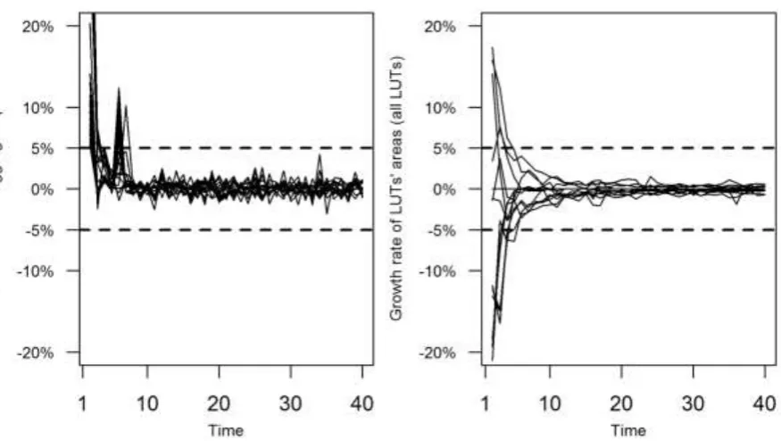
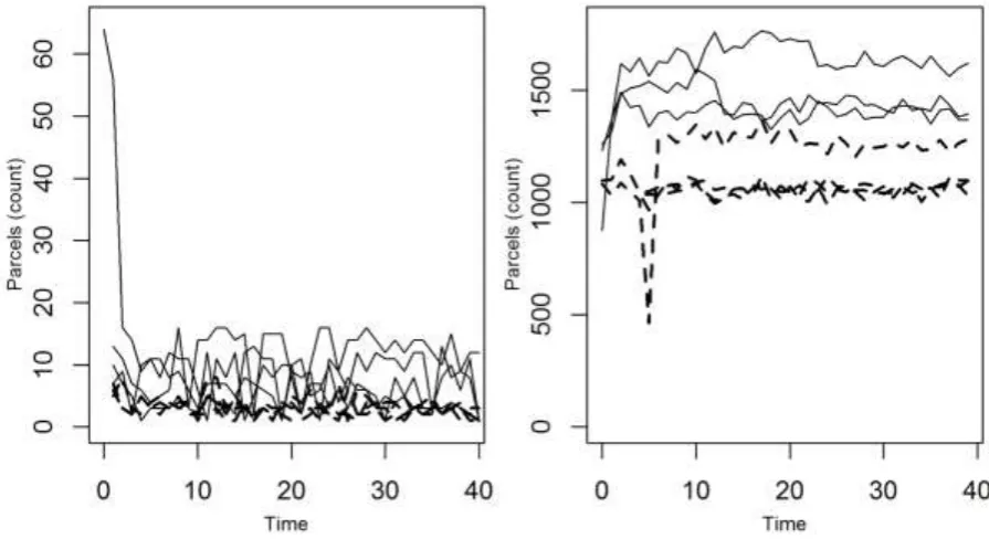
The long run is assumed to start when the change in aggregate actual profit and land use become negligible (figure 5 below). However, absolute stagnation was never observed with negligible growth prevailing even after a large number (500) of iterations. The long run is assumed to start when aggregate profit has grown for less than 5% in the last five consecutive steps. All simulations reach that point at t = 40 at the latest (but generally well before that, see figure 5). This is, therefore, the reference step for computing long-run causal effects. The rationale for basing analysis on the long run relates to the fact that agents' best responses to policy instruments are observable only after LUT portfolios were optimized. The latter is indicated by profit and landscape stagnation, given the gradual improvement approach farmers follow (section 3.2.4 above). It should also be highlighted that it is in such period that constraints are less stringent, being them either wealth or data on accidental fires, and then response to policy becomes mainly a matter of choice.

The policy instruments can be implemented in multiple “intensity levels”, as varying magnitudes of the fine and the subsidies. The set of intensity levels considered in simulations is L = {0.1,0.2,…,1}. All monetary values in the model are expressed as shares of the (landscape-wide) maximum parcel-level profit. Thus, a fine (subsidy) of $0.1/hectare reduces (increases) the profit yielded by a parcel in exactly 10% of the maximum parcel-level profit.

3

16 In summary, the long run causal effect on the v-th outcome variable of the p-th instrument implemented in the l-th intensity level is δvp,l(t = 40) = Wv0(t = 40) -Wvp,l(t = 40), with the superscript “0” indicating the baseline simulation and W the level of the outcome variable. The three outcome variables considered are counts of parcels with a particular type of fire among (i) accidental fires, (ii) reckless fires and (iii) agricultural fires (reckless and controlled fires). Conclusively, the long run causal effects capture avoided fires of the three kinds detailed.

Two of the instruments, C&C and mechanization, have a reach which is limited, in the spatial and social dimensions respectively. In contrast, all farmers were exposed to the two conservation instruments. To tackle different treatment groups, results are also presented for smallholders (farm size not above 200 hectares, which is the limit for mechanization) and medium-to-large landholders (farm area above 200 hectares; also denoted as “medium-to-large”).

Figure 5 Stagnation of aggregate profit (left) and landscape (right) before the long run (t = 40), all simulations.

4.1.2 Sensitivity tests

17 ordering of LUTs, leading to simulations that are excessively different from the one whose results are evaluated in the main text (next subsection). To avoid this, all parameters of a class (risk or LUT) receive the same percent shock. The results are found in SM.3.

4.2 Short-run dynamics

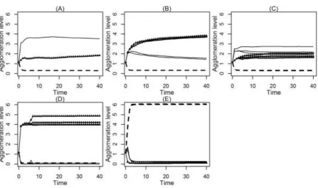
The short-run dynamics of the model is synthesized by the trend of a single workhorse state variable, the average number of neighboring parcels with a given LUT. This measure for the agglomeration level determines the expected profits of the LUTs (section 3.2.4) and, therefore, the long-run LUT portfolios. The short run dynamics is a history of a race that is won in the very beginning (figure 6). The initial condition allocates the four LUTs randomly with uniform probability to non-forested parcels, resulting in an average agglomeration level of 1.10 parcels for agricultural LUTs4. For such agglomeration level, the LUT that yields the highest expected profit quickly becomes dominant in the baseline simulation (around t = 5) and remains so in the long run. Such is the case of reckless fire, which is the most profitable LUT up to an agglomeration level of 2 parcels (figure 4).

In the baseline, it is observed a feedback in which the agglomeration and spatial diffusion of reckless fire reinforce each other. Such feedback is broken by policy instruments right in the first time step. Fines and subsidies work as exogenous shocks on the expected profit yielded by LUTs, overturning the advantage of reckless fire and opening space for the other two agricultural LUTs. In all policy simulations except Mechanization, which directly incentivizes fire-free, it is controlled fire that dominates in the long run (figure 6). Conservation, the only instrument without a restriction or subsidy against reckless fire, proved to be the least effective in reverting the LUT’s dominance.

The baseline trend is consistent with studies advocating the existence of a self-sustaining dominance of fire use (fire lock-in) in the Brazilian Amazon, with emphasis in the dependence of smallholders on slash-and-burn agriculture (Costa, 2004, Nepstad et al, 2001, section 2, Cammelli, 2014, section 4.2.3). There are also widespread claims in the literature that, as our policy simulations show, intervention is needed in order to break the lock-in. This belief, adhering to the originally proposition of technological lock-in (Arthur, 1989), is also confirmed by research on fire use. In Börner’s et al (2007) simulations, policies promoting fire-free technologies and also taxing slash-and-burn proved successful. More recently, among smallholders participating in a PES program in Amazonas state, Börner et al (2013, p.56), found weak evidence of a reduction in deforestation, which probably means that the rate of expansion of slashed and burned area decreased. Van Vliet et al (2013) argue that policy based on conditional cash transfers has restrained shifting cultivation.

A novelty of our paper is the process driving the agricultural fire lock-in, which connects the initial land use condition (an historical event in the sense of Arthur, 1982) with agglomeration induced by scale economies (spatially-explicit processes which create increasing returns also in line with Arthur, 1989).

4

18 Figure 6 Agglomeration level of agricultural LUTs, all simulations (baseline (A), C&C (B), Conservation (C), Conservation+ (D), Mechanization*(E))

Caption: solid line = reckless fires, solid line with triangles = controlled fires, dashed line = fire-free agriculture. Agglomeration level in the vertical axis. Note: For mechanization, only parcels belonging to smallholdings (the instruments’ target) were considered.

4.3 Analysis of results

Five main “potential lessons” synthesizing what could be learnt from the results are here presented and discussed. By “lessons” it is not meant recommendations to be put in practice but rather hypotheses about the impacts and limits of policy instruments whose validity is yet to be tested using empirical data. These potential lessons are robust to multiple values of parameters, as attested by sensitivity analysis (SM.3).

4.3.1 Relative effectiveness of instruments

19 Effectively, the coarse spatial resolution of fire-monitoring frees smallholders from costly fines. Smallholders are only impacted by the C&C instrument indirectly, through spatial spill-overs of the reactions of medium-to-large landholders, an effect with negligible magnitude (figure 7). This yields the first potential lesson (PL).

(PL 1) If fire monitoring is based on remote sensing with low spatial resolution, banning reckless fire may exert low impact on accidental fires and on total fire use. Moreover, smallholders may remain unexposed to enforcement.

This finding echoes that of Godar et al (2014), who show that smallholders are the social group least impacted by Brazilian deforestation policy due to the limited spatial resolution of deforestation monitoring and the political acceptability and cost-effectiveness . Additionally, Assunção et al (2013) argue that higher resolution monitoring would increase the effectiveness of deforestation policy. Finally, Börner et al (2015) found no statistically significant impact of field-based enforcement on deforestation of patches below 25 hectares, which is the current resolution of real time monitoring of deforestation in Brazil.

In this study the mechanization subsidy performed best for all three outcome variables (figure 7), considering only the social group exposed to it, namely, smallholders. Stimulating farmers to stop using fire, whether in a reckless or controlled manner, seems to be the most effective path to reduce accidental fires and, obviously, total fire use. Only in avoiding reckless fires, mechanization is matched by any other instrument, in particular conservation+. The latter is the only other incentive instrument that restricts fire use but, in contrast with mechanization incentives, it does not compensate for compliance. Consequently, we conclude that:

(PL 2) Subsidies to shift from fire-based to mechanized agriculture may prove more effective in reducing fires than either C&C or conservation instruments.

Effectiveness of the incentive was proportional to how directly it impacted fire use, as revealed by the impact rank of the three incentive instruments, which, for most of outcome variables and intensity levels, was, in decreasing order, mechanization, conservation+ and conservation (considering only groups exposed to the instrument). Conservation is the least direct instrument due to the absence of clauses regulating fire use, whereas conservation+ prevents reckless fire use only by incentivizing farmers to avoid converting 10 year old forest to reckless fires. Mechanization is the most direct instrument. Such results are compatible with the claim by Ferraro and Kiss (2002) that payments are most effective whether directly remunerating the desired environmental benefit.

The almost negligible impact of C&C policy on smallholders (Table 4) do not mean ineffectiveness but instead reveal negligible exposure (treatment by policy) driven by limited enforcement. Analogously, the negligible impact of mechanization subsidies on medium-to large-farms is caused by the focus on smallholders.

20 incentives. The LUT choice is discrete and once a LUT is promoted to the top of the profit rank, further increasing its profitability exogenously does not change the rank and, therefore, incentives remain the same. This is consistent with theory which sustains that policy can only have its effectivity increased while there are open opportunities to change incentives (e.g. Becker, 1968). This “decreasing return” of instruments is especially relevant given that neither of them could reduce the accidental fire rate below 12% of the landscape from a baseline level of 26%. Consequently:

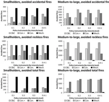
(PL 3) Command-and-control and incentive-based instruments may be effective in altering land use and fire level, but such effectiveness is limited.

Figure 7 Long run causal effects of instruments*, vertical axis: avoided fires measured as counts of parcels (hectares); horizontal axis: instrument intensity (fine or subsidy)

Caption: “C&C” stands for command-and-control policy and “Con+”, “Con” and “Mech.” for the three incentive-based instruments (section 2.2). In each plot, the effects are shown for intensity levels from 0.1 to 1. 4.3.2 Side-effects of instruments

21 fire is mandatory but not subsidized, farmers face the income loss imposed by the restriction as an opportunity cost of signing a conservation+ contract. Second, reckless and controlled fires are, respectively, the first and second most profitable LUTs in the initial condition of all simulations (section 4.2). Therefore, to compensate for the opportunity cost, reckless fire use and also the lower-ranked fire-free are replaced by controlled fire use.

The compensation through disproportionate expansion of controlled fire use (see figure 6) can be understood by remembering that agglomeration of a LUT is driven by scale economies. Hence, the larger the area of controlled fire is, the more diluted is the fixed cost it incorporates. Making fire-breaks is an example of a fire control measure with fixed cost when aimed at protecting land uses outside the areas to be treated with fire. The relevance of this example is attested by the positive correlation between firebreak investment and value of land use under risk found by Bowman et al. (2008), who analysed data from a protected area in our study region, Santarém.

If agricultural fires are seen as undesirable for other reasons beside accidental fire risk (e.g. smoke and derived air pollutants and GHGs, and soil degradation), results suggest that forest conservation payments are not the most efficient instruments to address the issue5. This is also true for C&C instrument as it considerably increased controlled fires (figure 6). Of course, a “conservation++” contract forbidding reckless fire and controlled fire could be designed, and it would probably be more effective at avoiding accidental fires, at least for farmers motivated to sign the contracts. However, the number of farmers entering the scheme would likely be smaller. This is supported by the fact that the total number of farmers willing to sign a forest conservation contract is smaller when reckless fire is forbidden and the payment is below 0.4/hectare (table 6). It is only above this value that the reckless fire restriction has no impact on the total number of signed contracts.

Summing up, the incorporation of restrictions to fire use into PES programs in the Brazilian Amazon is necessary to assure an acceptable "return" for the payments, i.e. the quality of conserved forest. However, the simulations suggest that farmers need to be compensated for the cost of complying with restrictions in order to achieve the double PES goals of an acceptable return and desirable geographical reach. Without this, policy-makers would have to accept both a relevant level of agricultural fires and a reduced amount of land kept as forest. This finding leads to the fourth potential lesson.

(PL 4) The conditioning of conservation payments on the prohibition of reckless fires may be effective to avoid subsidized forest from being accidentally burned. However, as a side-effect, controlled fires may increase considerably and the whole area of conserved forest might fall. The practical relevance of this potential lesson is attested by Leiva-Montoya’s (2013) interviews with participants of the ongoing PES program “Bolsa Floresta”. He found that 77% of the interviewees judged the household-targeted payment insufficient to cover the costs of compliance with deforestation and fire use restrictions. In a relevant number of

5_{Moreover, in practice, during extreme droughts, as observed, for instance, in 2005, 2007 and 2010 (Stosic et}

22 programs (see Pattanayk et al. 2010, Appendix table 2), compliance monitoring is imperfect and detection of violations is probabilistic. If payments partially cover compliance cost, theoretically (see Ferraro, 2008, p.811), partial compliance would tend to prevail at a level in which its cost balances payments.

Still, that fires may undermine environmental gains brought by incentives to avoid deforestation is argued by Friess et al (2015), Aragão and Shimabukuro (2010) and Barlow et al (2012). Their results show a clear need to introduce fire restrictions in REDD programs. This is already taking place in the Juruá and Rio Negro protected areas of Amazonas (Börner et al, 2013, p.18, Leiva-Montoya, 2013 p.38), where payments for forest conservation are conditional on the adoption of fire control measures (e.g. firebreaks ) and on norms restricting the frequency and extent of burning (Börner et al, 2013).

Now, turning to the mechanization instrument, it quadruples fire-free area, promoting the LUT to a degree of diffusion (16%) that has no parallel in the other simulations (figure 6). It is also observed a significant shift from fire-based to fire-free agriculture. In the baseline, the area occupied by the former is 18 times larger than the area occupied by the latter. However, with a mechanization subsidy of R$0.4, based area is only 3 times larger than that of fire-free.

Even with such major impact on the fire-free area, only marginal unwanted indirect land use change could be found at farms exposed to the subsidy (see SM.3 table SM.3.13). In the case of the mechanization instrument, the unwanted indirect land use change is the replacement of forests by fire-free, which, even though not incentivized, is not ruled out by the contract and could theoretically happen due to the high agglomerative potential of fire-free. But the side-effect is not driven by spill-overs. It is, indeed, very straightforward. Smallholders explore the possibility of converting forest to fire-free in the first period in order to start receiving the mechanization subsidy in the third period. It is exactly what happens in the sensitivity simulation with highest share of indirect land use (table SM.3.13).

This side-effect should not be thought as irrelevant for being caused by a caveat in contractual rules. In theory, the issue could be solved by not remunerating the keeping of free, except in parcels where the LUT replaced based agriculture. However, the fire-based agriculture currently replaced may have taken the place of forest. To solve the problem in practice, recently deforested parcels should be not remunerated, but, still, the definition of "recently" may be a matter of dispute.

23 can be considerably mitigated if only a particular land use change, which does not, obviously, coincides with deforestation, is accurately subsidized. Synthesizing the discussion:

(PL 5) Indirect deforestation induced by mechanization subsidy may be kept low if the conversion of forests to mechanized agriculture is not direcly subsidized.

However, mechanization may also have negative social and environmental impacts depending on how it is introduced. If cash flow and credit access are below the levels required for regular and minimum fertilizer application, income will fall in the short term. It will also fall in the long term when soils worn-out by slash-and-burn are not rehabilitated before tractor introduction, which can only lead to further degradation (Reichert et al., 2014). A mechanization subsidy, thus, has to cover the cost of sustainable soil management required by tractor introduction.

Figure 8 Counts of forested parcels accidentally burnt, only subsidized parcels (left) and all parcels (right), Conservation (solid line) and Conservation+ (dashed) contracts.

Table 6 [here] Table 7 [here]

24 Without public action, the current number of ignitions by farmers, combined with increased drought hazard and fire-prone vegetation, seems set to lead to disastrous wildfires, biodiversity loss, GHG emissions, and the spread of health-damaging pollutants (Balch, 2014, Jacobson et al., 2014, Malhi et al., 2009, Davidson et al, 2012). Alarmingly, there is no clear evidence that current Brazilian fire policies are promoting a relevant reduction of Amazon fires (see Sorrensen, 2009, Carmenta et al., 2013, Arima et al., 2007 and Costa, 2004). To better understand the impacts and limitations of policy options, we developed and applied an analytical tool to a small fraction of the Brazilian Amazon, identifying five potential lessons. The instruments evaluated cover a relevant fraction of the menu of choices in practice faced by policymakers, ranging from a negative incentive to abandon only reckless fires (C&C instrument), where compliance cost is fully borne by landholders, to a positive incentive where government fully pays for the cost of ceasing to use both reckless and controlled fires (mechanization).

For the social groups exposed to them, all policy instruments proved effective in overturning the predominance of highly profitable and risky fire use and also in decreasing accidental fires. However, none of them were free from imperfections. A ban enforced with fines performed worse than incentive-based instruments due to inadequate monitoring of compliance, leaving smallholders immune to sanctions. Forest conservation subsidies avoided deforestation but not forest degradation by fire. Such subsidies, when made conditional on the avoidance of reckless fires, did ensure reduced forest degradation, but the price paid was increased controlled fire use and less avoided deforestation. A subsidy to shift from fire-based to fire-free agriculture was the most effective instrument to avoid fire use and accidental fires, but it indirectly incentivised deforestation. Furthermore, for most intensity levels, the instruments that were more effective at reducing deforestation were not more effective at reducing fires, and vice versa (table 7). Thus, even within the wide spectrum of policy options examined, an instrument to achieve, with high impact, the double goal of total fire reduction and forest protection could not be found (except for intensity levels 0.1 and 0.2, see table 7). This is likely due to the impossibility of achieving multiple goals with a single instrument, as the Tinbergen rule proposes (Knudson, 2009).

Finally, due to the artificial nature of the data generated by the simulations, the results obtained are far from definitive, and only a point of departure for empirical research aimed at refuting the lessons learned. Nevertheless, the study has contributed a crucial first step towards analysing the impacts of policy on Amazonian fires by providing clear-cut hypotheses for further study.

25 (SM.1) and results involving them can only be extrapolated, with care, for the subgroup of farms from between 100 and 200 hectares.

26 Appendix A ODD+D description of the model

I.Overview I.i Purpose

I.i.a What is the purpose of the study? The model is a tool to build knowledge on the impacts and limitations of command-and-control and incentive-based policy instruments designed to control agricultural and accidental fires in the Brazilian Amazon.

I.ii.b For whom is the model designed? Researchers of Amazon fires and policy-makers I.ii Entities, state variables, and scales

I.ii.a What kinds of entities are in the model? Four kinds of entities. First, the decision makers that manage land, called "farmers". Second, spatial units, called "parcels". The latter kind of entity does not make decisions, but executes natural processes (forest growth, forest degradation, etc.) and is employed by farmers to process calculations required by land use and technology (LUT) choice. Third, an observer entity, called "nature", decides which parcels accidentally burn. Fourth, an observer entity, called "government", sanctions reckless fires in the command-and-control policy scenario and offers and monitors voluntary contracts in the incentive-based policy scenarios.

I.ii.b By what attributes (i.e. state variables and parameters) are these entities characterized? (immutable initial conditions, which are equal across all simulations, are denoted by "[i.i.c]"; state variables, by “[s]”).

(1) Farmers are characterized by: (1.a) Farm, i.e., set of parcels controlled [i.i.c]; (1.b) LUT portfolio choice [s]; (1.c) wealth or accumulated stock of whole-farm profits [s]; (1.d) point estimates for risk parameters [s]; (1.e) accumulated local data on fires and LUTs [s]; (1.f) contract status (regarding incentive-based instruments) [s];

(2) Parcels are characterized by: (2.a) location [i.i.c]; (2.b) farmer in control [i.i.c]; (2.c) physical suitability [p]; (2.c) LUT [s]; (2.d) age of forest, (2.e) above-ground forest biomass (AGB) [s]; (2.f) inclusion in enforcement-effective zone [i.i.c]; (2.g) whether accidentally burned or not [s];

(3) Nature is characterized by: (3.a) true risk parameters [i.i.c]; (3.b) values for standard Gaussian disturbance behind accidental fires [s];

(4) Government is characterized by: (4.a) Active policy instrument [i.i.c]; (4.b) level of intensity for policy (value of fine or subsidy) [i.i.c].

27 I.ii.d If applicable, how is space included in the model? With a two dimensional flat landscape whose basic unit is an autonomous processing unit referred as "parcel". The model is spatially explicit and operates in a landscape whose division among private owners comes from real data (Rural Environmental Land Registry, SM.1) and remains fixed across simulations. The initial condition for land use is also partially defined by data.

I.ii.e What are the temporal and spatial resolutions and extents of the model? One time step represents one year, simulations were run for 40 years, one grid cell represents 1 ha and the model landscape comprises 100 x 100 hectares.

I.iii Process overview and scheduling

I.iii.a What entity does what, and in what order? (names of procedures are preceded by an indication of the entities that run them, as follows: [F] for farmer, [P] for parcel, [G] for government and [N] for nature)

(A) In baseline and command-and-control policy simulations, the following nine modules are executed in the following order: [P&F] calculate-profit, [P&F] implement-LUT-portfolio, [F] LUC-cost-account, [N] define-burned-parcels, [G] sanction-rulebreakers, [F] calculate-actual-profit, [F] risk-parameters, [F] store-LUT-portfolio-in-memory, [P] update-forest-age-after-burn.

The first iteration differs only regarding the absence of the procedure "update-risk-model-parameters" (since farmers have no local data at t = 0).

(B) In incentive-based policy simulations, the same procedures are processed together with two extra procedures: (i) [F] subsidy-payment-account which is deployed right after "implement-LUT-portfolio" and; (ii) [F] update-contract-duration, deployed right after "LUC-cost-account". In procedure (ii), decisions on signing, keeping and renewing a subsidy contract are made. One additional peculiarity of incentive-based simulations is that the "calculate-profit" procedure is subdivided in two sub-procedures, one calculates profit without imposing compliance with contract rules and the other forces compliance (B.1 and B.2 of appendix B).

II. Design concepts

II.i.a Which general concepts, theories or hypotheses are underlying the model’s design at the system level or at the level(s) of the submodel(s) (apart from the decision model)? What is the link to complexity and the purpose of the model?

28 Bateman, 2011); Parcel-level heterogeneity and spatial externalities of land uses (Irwin and Bockstael, 2001, Parker and Meretsky, 2004).

II.i.b On what assumptions is/are the agents’ decision model(s) based?

Farmers are boundedly rational and choose LUT portfolio in the basis of a local (parcel-level) optimization procedure adjusted to incorporate farm-level information; Current wealth is a limiting factor of LUT portfolio change due to cost of land use change; It is necessary to form expectations on the LUTs to be developed at third-party parcels in the neighborhood of farm boundaries. This is done by assuming that previous step LUTs will be kept; Farmers are ignorant of true risk parameters and the value of the random disturbance behind accidental fires; Data for estimating risk parameters is collected locally and accumulated stepwise over time.

II.i.c Why is a/are certain decision model(s) chosen? There are two reasons. First, standard global optimization, i.e., finding the best among all possible portfolios is highly computing-intensive. Once there are four LUTs, the number of alternative portfolios is equal to four elevated to a power equal to farm’s area. For a 30 hectare farm, the smallest farm size in the model, the number of potential portfolios has an order of magnitude of 1018.Second, empirical studies of Amazon farmers' behavior show that land management decisions are driven by parcel-scale factors and limited by capital/wealth (Deadman et al., 2004, Sorrensen, 2000 and 2004, Moran et al., 2002, Scatena et al., 1996, McCraken et al. 2002). In particular, econometric results (e.g., Pfaff, 1999, Pfaff et al., 2007), reveal that proximity to roads, urban centers and low inclination of land, the three variables captured by the model's physical suitability, positively influence the conversion of forests to agriculture. This causality is the basis of the model's wealth allocation principle of giving priority to parcels whose costly conversion is, due to physical factors, more profitable.

29 II.i.e At which level of aggregation were the data available? Land use change cost data: at the level of production factors (man-days, input quantities/output, etc.), see SM.2; Forest growth model: at the parcel (stand) level; Land property and initial land use data: parcel level, 30 m resolution data.

II.ii Individual Decision Making

II.ii.a What are the subjects and objects of decision-making? On which level of aggregation is decision-making modeled? Are multiple levels of decision making included? Farmers decide on the allocation of parcels among alternative LUTs. Nature decides, based on LUT configuration, which parcels accidentally burn. No other entity is capable of decision making. Government only implements pre-defined rules regarding farmer sanctioning.

II.ii.b What is the basic rationality behind agents’ decision-making in the model? Do agents pursue an explicit objective or have other success criteria? Farmers are boundedly rational and seek the portfolio that maximizes whole-farm expected profit. Nature is substantively rational in the sense it does not face barriers for gathering and processing information but has no particular goal. Government does not follow a decision model, it simply implement rules (non-deliberate action).

II.ii.c How do agents make their decisions? Se II.ii.a and II.i.b above and appendix B.

II.ii.d Do the agents adapt their behavior to changing endogenous and exogenous state variables? And if yes, how? ("exo" stands for exogenous variables and "endo" for endogenous).

Yes, farmers adapt to: (1) LUTs of third-party parcels (exo), which create profit and risk spill-overs that influence LUT allocation at the boundary of farms; (2) Knowledge of the true process behind accidental burns, measured by accumulated local data on LUTs and accidental fires (endo. and exo.). This drives change of LUT portfolios due to changed perceived risk associated with LUT mosaics; (3) Own-wealth (endo.), which, being updated by whole-farm profit, becomes less stringent as a constraint on chosen portfolios; (4) Forest growth (exo.), which engenders profit and risk spill-overs that may lead farmers to reconsider LUT portfolios and their statuses regarding conservation contracts.

II.ii.e Do social norms or cultural values play a role in the decision-making process? No, there is no direct interaction among farmers and institutions are abstracted (apart from policy which is immutable during simulations).

II.ii.f Do spatial aspects play a role in the decision process? Yes, a crucial role through spill-overs of parcel-level risk and profit and also by signaling to agents that accidental burns emerge (also) from particular spatial configurations of LUTs.

30 II.ii.h To which extent and how is uncertainty included in the agents’ decision rules? Agents face two sources of uncertainty while searching for the best LUT portfolio. First, the best LUT portfolio of neighbors is unknown. Second, there is the uncertainty related with the true generating process behind accidental burns coming from (i) ignorance of the true risk parameters and (ii) randomness of unobservables. While (i) is mitigated with the accumulation of local data, (ii) is irreducible, and, therefore, accidental burns are always uncertain events in the model, even after farmers’ point estimates for risk parameters have become sufficiently close to true values.

II.iii Learning

II.iii.a Is individual learning included in the decision process? How do individuals change their decision rules over time as a consequence of their experience? Yes, farmers learn about the true process behind accidental burns, as described in appendix B, B.13.

II.iii.b Is collective learning implemented in the model? No. II.iv Individual Sensing

II.iv.a What endogenous and exogenous state variables are individuals assumed to sense and consider in their decisions? Is the sensing process erroneous? Farmers sense the risk of accidental burns associated with LUT configurations. This sensing is improved with local data accumulation but may prove wrong when estimates of risk parameters do not match the true values which are known only by nature.

II.iv.b What state variables of which other individuals can an individual perceive? Is the sensing process erroneous? Farmers observe the behavior of neighbors, but exclusively with regard to LUTs allocated to parcels bordering their own farm. On the basis of this, they try to forecast current LUTs of such proximate third-party parcels, but such forecasts may prove wrong.

II.iv.c What is the spatial scale of sensing? Local, parcel scale, restricted to own-parcels and third-party parcels within 100 meters from farm boundaries.

II.iv.d Are the mechanisms by which agents obtain information modelled explicitly, or are individuals simply assumed to know these variables?

(1) Farmers: (1.a) The mechanism of accumulation of information on accidental fires and LUTs is modelled explicitly. It is assumed that farmers know the specification of the true function behind accidental burns, which is a standard probit and estimate the parameters with local data; (1.b) Information on LUTs of proximate third-party parcels is obtained through direct observation;

(2) Nature and government know all the information they need to act.