Maximum likelihood estimation for multiscale Ornstein Uhlenbeck processes

warwick.ac.uk/lib-publications

Original citation:

Zhang, Fan and Papavasiliou, Anastasia. (2018) Maximum likelihood estimation for

multiscale Ornstein-Uhlenbeck processes. Stochastics.

Permanent WRAP URL:

http://wrap.warwick.ac.uk/97268

Copyright and reuse:

The Warwick Research Archive Portal (WRAP) makes this work by researchers of the

University of Warwick available open access under the following conditions. Copyright ©

and all moral rights to the version of the paper presented here belong to the individual

author(s) and/or other copyright owners. To the extent reasonable and practicable the

material made available in WRAP has been checked for eligibility before being made

available.

Copies of full items can be used for personal research or study, educational, or not-for profit

purposes without prior permission or charge. Provided that the authors, title and full

bibliographic details are credited, a hyperlink and/or URL is given for the original metadata

page and the content is not changed in any way.

Publisher’s statement:

“This is an Accepted Manuscript of an article published by Taylor & Francis in Stochastics on

28/01/2018 available online:

https://doi.org/10.1080/17442508.2018.1424853

A note on versions:

The version presented here may differ from the published version or, version of record, if

you wish to cite this item you are advised to consult the publisher’s version. Please see the

‘permanent WRAP URL’ above for details on accessing the published version and note that

access may require a subscription.

Maximum Likelihood Estimation for Multiscale

Ornstein-Uhlenbeck Processes

Anastasia Papavasiliou

Department of Statistics

University of Warwick, UK

and

Fan Zhang

School of Banking and Finance

University of International Business and Economics, China.

September 11, 2017

Abstract

We study the problem of estimating the parameters of an Ornstein-Uhlenbeck (OU) process that is the coarse-grained limit of a multiscale system of OU pro-cesses, given data from the multiscale system. We consider both the averaging and homogenization cases and both drift and diffusion coefficients. By restrict-ing ourselves to the OU system, we are able to substantially improve the results in [23, 21] and provide some intuition of what to expect in the general case. In particular, in the homogenisation case we derive optimal rates of sub-sampling, proving the conjecture in [23].

Keywords: multiscale diffusions, Ornstein-Uhlenbeck process, parameter estimation, maximum likelihood, subsampling.

1

Introduction

A necessary step in statistical modelling is to fit the chosen model to the data by in-ferring the value of the unknown parameters. In the case of stochastic differential equations (SDE), this is a well studied problem [6, 16, 24]. However, quite often, data actually comes from a multiscale SDE whilst we want to model its coarse-grain ap-proximation. This phenomenon has been observed in many applications, ranging from econometrics [1, 2, 20] to chemical engineering [5] and molecular dynamics [23]. In this paper, we study how this inconsistency between the coarse-grained model that we fit and the microscopic dynamics from which the data is generated affects the estima-tion problem.

The problem of estimating the drift and variance parameters of an Ornstein-Uhlenbeck (OU) process is a standard one. Statistical inference for diffusions is a well-developed

area and the remaining challenges mainly concern the exact computation of the likeli-hood. In the case of the OU process, computing the exact likelihood is straight forward. In the context of the OU process, the problem has been extended to the case where the differential equation is not exactly a diffusion. For example, in [15], the authors studied properties of usual drift estimator for scalar OU processes driven by fractional Brownian motion. Further more detailed studies extended the results to stronger con-sistency and asymptotics under various assumption: such as in [9], authors discussed the asymptotics of the drift estimators for an OU process driven by fractional Gaussian processes, sub-fractional and bi-fractional Brownian motions, with infinite observation with Hurst parameterH ∈(0,1); and [18] studied strong consistency and asymptotic normality for the usual drift estimator for infinite dimensional fractional OU process, under the assumption that Hurst parameterH ≥1/2.

Another extension the problem was into considering the observation process as component of a multiscale process, converging in some limit to an OU process. This is the problem we are interested in. It has also been discussed in several papers. In [3, 4], the authors compute the bias between the estimators corresponding to multiscale and approximate Ornstein-Uhlenbeck (OU) process, as a function of the subsampling step sizeδand the scale factor. However, their approach is somewhat ad-hoc and limited to scalar systems.

We consider the case where the multiscale system is an OU process, where the av-eraging and homogenization principles still hold. We look at the MLE estimators of both the drift and diffusion coefficients of the limiting system and study their properties in the case when data comes from the multiscale system. In the averaging case (section 2), we show that the estimators are consistent and asymptotically normal. However, the homogenisation case (section 3) is much more complicated as estimators are not con-sistent. To construct consistent estimators, one needs to subsample the data. We show that the estimators will be consistent in that case. However, proving asymptotic normal-ity is much more involved and beyond the scopes of this paper. Our approach is similar to that in [23, 21]. In the first, the authors study a similar problem for slightly more general models but get weaker results. In the latter, the authors study the behaviour of the drift likelihood of the limiting system for data coming from the multiscale system. Finally, let us note that MLE estimators for diffusions are known to have prac-tical limitations. In particular, the drift estimator requires a long horizon to achieve satisfactory precision while the diffusion estimator needs very fine scale data. In the homogenisation case that we study, there is the additional issue of subsampling the data at a sampling rate that depends on normally unknown separation of scales variable. However, we believe that the behaviour that we observe is inherent to the problem of mismatch between the model and data and not the estimators and thus have chosen a set-up where analysis can be done in detail.

We present the exact set-up and main ideas below. Let(Ω,F,{Ft}t>0,P)be a

filtered probability space, andU, V be two independent Brownian motions defined on this space. We consider multiscale systems of SDEs of the form

dx t

dt = a11x

t+a12yt+√q1

dUt

dt , x

_=x

0 (1a)

dy t

dt =

1

(a21x

t+a22yt) + r

q2

dVt

dt , y

_=y

or

dx t

dt =

1

(a11x

t+a12yt) + (a13xt+a14yt) +√q1

dUt

dt , x

_=x

0 (2a)

dy t

dt =

1

2(a21x

t+a22yt) + r

q2

2

dVt

dt , y

_=y

0 (2b)

wherex0, y0are random variables,(a11, a12, a13, a14, a21, a22)are real constants that

will be required to satisfied certain relationships to be specified later which guarantee ergodicity andq1, q2are positive real constants. The variable >0denotes scale

sep-aration and we will consider the behaviour of the above system in the limit→0. We refer to equations (1) and (2) as the averaging and homogenization case, respectively and we denote byρ(x, y)their invariant distribution, when this exists. In both cases

and under certain conditions,(x

t)0≤t≤T converges as→0to the solution of

dXt

dt = ˜aXt+

√

σdWt

dt , (3)

for appropriate ˜a ∈ Randσ ∈ R+ and in a way to be made precise later, for W

also Brownian motion defined on the probability space. Our goal will be to estimatea

andσ, assuming that we continuously observe(x

t)0≤t≤T from (1) or (2). It is a well

known result (see [6, 19]) that, given(Xt)0≤t≤T, the maximum likelihood estimators

forais

ˆ

aT =

Z T

0

XtdXt !

Z T

0

Xt2dt

!−1

. (4)

If(Xt)0≤t≤Tis discretely observed, then the estimator ofσis the discretised Quadratic

Variation

ˆ

σδ=

1

T

N−1

X

n=0

X(n+1)δ−Xnδ

2

(5)

which converges inL2toσasδ→0. Our approach will be to still use the estimators

defined in (4) and (5), replacingXtby itsxt approximation coming from the

multi-scale model and then studying their asymptotic properties. In section 2, we discuss the averaging case while in section 3 we study the homogenization case.

We shall discuss problems in scalars for simplicity of notation and writing. How-ever, the conclusions can easily be extended to finite dimensions. We will usec to denote an arbitrary constant which can vary from occurrence to occurrence. Also, for the sake of simplicity we will sometimes write x

n (oryn,Xn) instead ofxnδ (resp.

y

nδ,Xnδ). Finally, note that the transpose of an arbitrary matrixAis denoted byA∗.

2

Averaging

We consider the system of stochastic differential equations described by (1) (averaging case), where(x

t, yt)∈ X × Y. We may takeX andYas eitherRorT. We make the

following assumptions:

Assumptions 2.1.

Let(Ω,_F,_{Ft}t>0,P)be a filtered probability space. We assume that

(ii) q1,q2are positive real constants;

(iii) 0< 1is the scale separation variable;

(iv) a22<0anda11< a12a−221a21;

(v) x0andy0are random variables, independent ofU, V andE x20+y20

<_∞.

These assumptions guarantee the ergodicity of system (1). In this case, the averag-ing limit of the system is given by the followaverag-ing equation (see [14]):

dXt

dt = ˜aXt+

√_q

1

dUt

dt (6)

where:

˜

a=a11−a12a−221a21 (7)

2.1

The Paths

In this section, we show that(x

t)0≤t≤T defined in (1) converges in a strong sense to

the solutionX0≤t≤T of (6). Our result extends that of [22] (Theorem 17.1) where the

state space_X is restricted toTand the averaging equation is deterministic. Assuming

that the system is an OU process, the domain can be extended toRand the averaging

equation can be stochastic. We prove the following lemma first:

Lemma 2.2. Suppose that(x

t, yt)0≤t≤T solves(1)and Assumptions 2.1 are satisfied.

Then, for finiteT >0andsmall,

E sup

0≤t≤T

(xt)2+ (yt)2

≈ O

log

1 +T

. (8)

Proof. Since(Ut)t≥0and(Vt)t≥0are independent, we can rewrite (1) in vector form

as

dx_t=axtdt+√qdWt (9)

where

x_t=

x t

y t

,a=

a11 a12 1

a21

1

a22

,q=

q1 0 0 q2

andWt= (Ut, Vt)is two-dimensional Brownian motion. Given the form ofa, it is an

easy exercise to show that its eigenvalues will be of order_O(1)and_O(1

). Therefore,

we define the eigenvalue decomposition ofaas

a=PDP−1withD=

λ1() 0 0 1

λ2()

,

whereλ1(), λ2()are both of orderO(1). Again, it is not hard to see that if(p1, p2)

is an eigenvector,_O(p

1) = O(λ()− 1

i p2), fori= 1,2depending on the

correspond-ing eigenvector. So, for the eigenvector correspondcorrespond-ing to eigenvalue of order_O(1), all elements of the eigenvector will also be of order_O(1)while for the eigenvector corre-sponding to eigenvalue of order_O(1/), we will have thatp

1∼ O(1)andp2∼ O().

Now, let us defineΣ=P−1q(P−1)∗. It follows that

Σ=

O(1) _O(1)

O(1) _O(1/)

We apply a linear transformation to the system of equations (9) so that the drift matrix becomes diagonal. It follows from [10] that

E

sup 0≤t≤Tk

x_tk2

≤Clog (1 + maxi(|(D)ii|)T)

mini(|(D)ii/(Σ)ii|)

, i∈ {1,2}.

Since the diagonal elements ofDandΣare of the same order andmaxi|(D)ii|= O(1

), we have

E

sup 0≤t≤Tk

x_tk2

=O(log(1 +T /)).

The result follows by expanding the vector norm.

Theorem 2.3. Let Assumptions 2.1 hold for system(1). Suppose that(x

t, yt)0≤t≤T

and (Xt)0≤t≤T are two solutions of (1) and (6) respectively, corresponding to the

same realization of the(Ut)t≥0process andx0=X0. Then,(xt)0≤t≤T converges to

(Xt)0≤t≤T inL2(Ω, C([0, T],X)). More specifically,

E sup

0≤t≤T

(xt−Xt)2≤c

2log

_T

+T

eT2.

Note that when the time horizonT is fixed finite, the above bound can be simplified to

E sup

0≤t≤T

(xt−Xt)2=O().

Proof. The first step in the proof will be to expand the slow variablex

tin (1a) in terms

of. In the OU case, we can get the expansion directly by solving fory

t in (1b) and

using the answer to replacey

tin (1a). Note that a more general approach that can be

applied to nonlinear systems is to use Poisson equations (see [22]). Solving (1b) fory

tgives

yt=−a−221a21xt− √

a−221√q2dVt

dt +a

−1

22

dy t

dt (10)

and replacingy

tby (10) in (1a) gives

dxt= ˜axtdt+√q1dUt+√a12a22−1√q2dVt+a12a−221dyt, (11)

wherea˜is defined in (7). It follows that

xt=x0+

Z t

0 ˜

axsds+√q1Ut+√a12a−221√q2Vt+a12a22−1(yt−y0).

Also, from the averaged equation (6), we get

Xt=X0+

Z t

0 ˜

aXsds+√q1Ut.

Lete()t=xt−Xt. By assumption,e()0= 0and

e()t=

Z t

0 ˜

Then,

e()2t ≤3

˜

a

Z t

0

e()sds

2

+ a12a−221

2

Vt2+2 a12a−221

2

(yt−y0)2

!

.

Apply Lemma 2.2, the Burkholder-Davis-Gundy inequality [22], H¨older inequality and Itˆo isometry on (12), we get

E

sup 0≤t≤T

e()2t

≤ c T

Z T

0

Ee()2sds+2log(

T ) +T

!

≤ c 2log(T

) +T+T

Z T

0

E sup

0≤u≤s

e()2uds !

.

By Gronwall’s inequality [22], we deduce that

E

sup 0≤t≤T

(e()t)2

≤c(2log(T

) +T)e

T2

.

2.2

The Drift Estimator

Suppose that we want to estimate the drift of the process(Xt)0≤t≤T described by (6)

but we only observe a solution(x

t)0≤t≤T of (1a) for some > 0. According to the

previous theorem,(x

t)0≤t≤T is a good approximation of(Xt)0≤t≤T, so we replace

(Xt)0≤t≤Tin the formula of the MLE (4) by(xt)0≤t≤T. In the following theorem, we

show that the error we will be making is insignificant, in a sense to be made precise.

Theorem 2.4. Suppose that(x

t, yt)0≤t≤T solves system(1), satisfying Assumptions

2.1. LetˆaT be the estimate we get by replacingXtin(4)byxt, i.e.

ˆ

aT =

Z T

0

xtdxt !

Z T

0

(xt)2dt

!−1

. (13)

Then,

lim

→0Tlim→∞E(ˆa

T −˜a)2= 0,

fora˜given by(7).

Proof. We define

I1(T) = 1

T

Z T

0

xtdxt and I2(T) = 1

T

Z T

0

(xt)2dt.

By ergodicity, which is guaranteed by Assumptions 2.1(iii) and (iv)

lim

T→∞I2(T) =E (x

∞)2

=C6= 0a.s.,

parameters under assumptions 2.1. Using the (11) expansion ofdx

tin terms of, we

get

I1(T) = aI˜ 2(T) + (14)

+ √q1 1

T

Z T

0

x

tdUt+√a12a−221√q2 1

T

Z T

0

x

tdVt+a12a−221 1

T

Z T

0

x tdyt.

From Itˆo isometry and ergodicity, we directly get that

E √q1 1

T

Z T

0

xtdUt

!2

=q1 1

T2

Z T

0

E(xt)2dt=

c T

and similarly,

E √a12a−221√q2 1

T

Z T

0

xtdVt

!2

=c

T.

Finally, using (1b), we break the last term of (14) further into

1

T

Z T

0

xtdyt=−

1

T

Z T

0

xt(a21xt+a22yt)dt− √_q

2

T

Z T

0

xtdVt

As before, we see that the last term will be of order_{O T}. By ergodicity, the first term converges inL2_asT

→ ∞

−_T1

Z T

0

xt(a21xt+a22yt)dt→E(x∞(a21x_∞ +a22y_∞)),

where, as before,(x

∞, y∞ )are random variable distributed according to the invariant

distributionρof system (1). We write the above expectation as

E(x_∞(a21x_∞ +a22y_∞)) =E(x_∞E((a21x_∞+a22y_∞ )|x_∞)).

Clearly, the limit ofρconditioned onx_∞is a normal distribution with mean−a−221a21x_∞.

Thus, we see that

lim

→0E(x

∞(a21x_∞+a22y_∞ )) = 0.

Putting everything together, we see that

lim

→0Tlim→∞(I1−˜aI2) = 0 in L

2

Since the denominatorI2ofˆaT converges almost surely, the result follows.

2.2.1 Asymptotic Normality for the Drift Estimator

We extend the proof of Theorem 2.4 to prove asymptotic normality for the estimator

ˆ

a

T. We will show that √

T aˆ

T −˜a+a12E x∞(a−221a21x_∞+y_∞ )→ N 0, σ2

in distribution, as T _{→ ∞}and compute the limit of σ2

as → 0. We start with

expansion (14). First we apply the Central Limit Theorem to the martingales (see [11]). We find that

√

T √q1 1

T

Z T

0

xtdUt !

→ N 0, σ(1,1)2

where

σ(1,1)2

=q1E[(x∞)2]

and

√

T √a12a−221√q2 1

T

Z T

0

xtdVt !

→ N 0, σ(1,2)2

asT_{→ ∞}

where

σ(1,2)2=q2(a12a−221)2E (x∞)2

.

As before, we further expand the last component of the expansion (14) to

J1=−

a12a−221

T

Z T

0

(a21x2t+a22xtyt)dt and J2=−

a12a−221√q2

T

Z T

0

xtdVt.

Once again, we apply the Central Limit Theorem for martingales toJ2and we find

√

T J2→ N 0, σ(2,2)2

asT → ∞

where

σ(2,2)2=(a21a22−1)2q2E (x_∞)2.

Finally, we apply the Central Limit Theorem for functionals of ergodic Markov Chains toJ1(see [7]). We get

√

T J1+a12E x∞(a−221a21x_∞+y_∞ )→ N 0, σ(2,1)2

asT _{→ ∞}, where with

σ(2,1)2

= Var (ξ(x∞, y∞)) + 2

Z ∞

0

Cov (ξ(x0, y0), ξ(xt, yt))dt,

where

ξ(x, y) =₋ a12a22−1a21x2+a12xy.

Putting everything together, we get that asT_{→ ∞},

√

T(I1(T)−aI˜ 2(T))→Z(1,1)+Z(1,2)+Z(2,1)+Z(2,2),

in law, where Z(i, j) _{∼ N}(0, σ(i, j)2

), for i, j = 1,2. Finally, we note that the

denominatorI2 converges almost surely asT → ∞toE (x∞)2

. It follows from Slutsky’s theorem that asT _{→ ∞},

√

T ˆaT −˜a+a12E x∞(a22−1a21x_∞+y_∞ )→ N(0, σ2),

where

σ2 =

E(Z(1,1)+Z(1,2)+Z(2,1)+Z(2,2))2

E((x_∞)2)2

.

It remains to computelim→0σ2. We have already seen thatσ(1,2)2 ∼ O()and

σ(2,2)2

∼ O(), so we don’t expectZ(1,2)andZ(2,2)to contribute to the limit.

Also,

σ(1,1)2 =q1E (x_∞)2→q1E X_∞2 =−q

2 1 2˜a,

where X∞ is distributed according to the invariant distribution of system (6). To

also an ergodic process with invariant distribution ρ˜ that converges as → 0 to N(0,_2˜q1_a)_{⊗ N}(0,₂q2_a22). Sinceξ(x, y) =₋a21x·y˜(x, y), it follows that

lim

→0Var (ξ(x

∞, y∞)) =a212

q1 2˜a

q2 2a22

.

In addition, as_→0, the processy˜(x

t, yt)decorrelates exponentially fast. Thus

lim

→0Cov (ξ(x0, y0), ξ(x

t, yt)) =a212Cov (X0, Xt) lim

→0Cov (˜y(x0, y0),y˜(x

t, yt))≡0

for allt_≥0. Ast_{→ ∞}, the process(x

t,y˜(xt, yt))also converges exponentially fast

to a mean-zero Gaussian distribution and thus the integral with respect totis finite. We conclude that the second term ofσ(2,1)2

disappears as→0and thus

lim

→0E(Z(2,1) 2

) =a212

q1q2 4˜aa22

.

Finally, we show that

lim

→0E(Z(2,1)Z(1,1)) = 0.

Clearly,Z(1,1)is independent ofy˜(xt, yt)in the limit, since it only depends on the

processes_{x

t}t>0and{Ut}t>0. So, lim

→0E(Z(2,1)Z(1,1)) = lim→0E(E(Z(2,1)Z(1,1)|x

t, t >0))

and

lim

→0E(E(Z(2,1)|x

t, t >0)) = 0

for the same reasons as above. Thus

lim

→0σ 2

=

4˜a2

q2 1

−q

2 1 2˜a+a

2 12

q1q2 4˜aa22

.

We have proved the following

Theorem 2.5. Suppose that (x

t, yt)0≤t≤T is a solution of system(1)satisfying

As-sumptions 2.1. LetaˆT be as in(13). Then,

√

T(ˆaT −˜a−µ)→ N(0, σ2),

where

µ→0 and σ2 → −2˜a+a212 ˜

aq2

a22q1

as _→0.

Remark 2.6. Note that in the case where the data comes from the multiscale limit and

for_→0, the asymptotic variance of the drift MLE is larger than that the asymptotic

variance of the drift estimator where there is no misfit between model and data. The

asymptotic variance of the drift MLE with data coming from the averaged system,(4),

1 2 3 4 5 6 7 8 −10

−5 0 5

log2(T) √ T

(ˆ

a

ǫ T−

E

(ˆ

a

ǫ T))

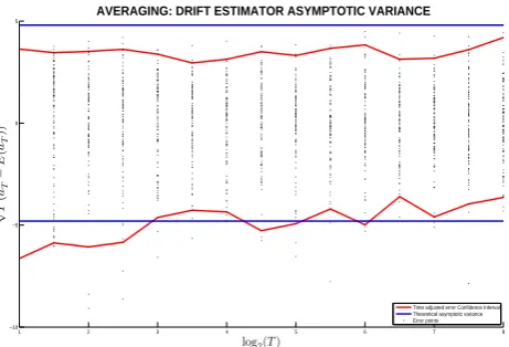
AVERAGING: DRIFT ESTIMATOR ASYMPTOTIC VARIANCE

Time adjusted error Confidence Interval Theoretical asymptotic variance Error points

Figure 1: The asymptotic variance of the drift estimator is constructed by plotting the distribution of the time adjusted errors√T(ˆa

T−E(ˆaT))for the following choice of

parameters: a11 = a21 = a22 = −1,a12 = 1,q1 = q2 = 2and = 2−9. Also,

T is sampled from21_to28_{. The blue lines are the theoretical bounds as described in}

Theorem 2.5, the red lines are the 2.5 and 97.5 percentiles from the simulated samples.

2.3

The Diffusion Estimator

Suppose that we want to estimate the diffusion parameter of the process(Xt)0≤t≤T

described by (6) but we only observe a solution (x

t)0≤t≤T of (1a). As before, we

replaceXtin the formula of the MLE (5) byxt. The following theorem states that the

estimator is still consistent in the limit.

Theorem 2.7. Suppose that(x

t, yt)0≤t≤T is the solution of system(1)satisfying

As-sumptions 2.1. We set

ˆ

qδ=

1

T

N−1

X

n=0

x(n+1)δ−xnδ

2

(15)

whereδ≤is the discretization step andT =N δis fixed. Then, for every >0

lim

δ→0E(ˆq

δ−q1)2= 0.

In addition, and in distribution

δ−12(ˆq δ−q1)

D

→ N(0,2q

2 1

T ) asδ→0.

The proof of the theorem is the standard proof of quadratic variation converging to the diffusion coefficient, as in the averaging case, the diffusion coefficient remains unaltered in the limit.

9 10 11 12 13 14 15 16 17 −10

−8 −6 −4 −2 0 2 4 6 8 10

−log2(δ)

δ

−

12(ˆ

q

ǫ δ−

E

(ˆ

q

ǫ δ))

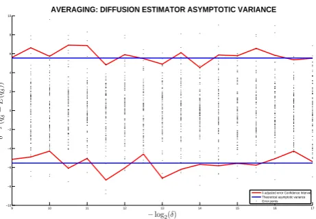
AVERAGING: DIFFUSION ESTIMATOR ASYMPTOTIC VARIANCE

δ adjusted error Confidence Interval Theoretical asymptotic variance Error points

Figure 2: The asymptotic variance of the diffusion estimator is constructed by plotting the distribution ofδadjusted errorsδ12 (ˆq

δ−E(ˆqδ))for the following choice of

param-eters: a11 =a21 =a22 =−1,a12 = 1,q1 =q2 = 2and= 2−9. Also,δsampled

from2−9_to2−17_{. The blue and red lines correspond to the theoretical and simulated}

95% confidence intervals.

3

Homogenization

We now consider the system of stochastic differential equations described by (2), for the variables(x

t, yt)∈ X × Y. We may takeX andYas either inRorT. Our interest

remains in data generated by the(x

t)0≤t≤T process.

Assumptions 3.1.

We assume that Let(Ω,F,{Ft}t>0,P)be a filtered probability space. We assume that

(i) (Ut, Vt)t≥0are independent Brownian motions;

(ii) q1,q2are positive real constants;

(iii) 0< 1is the scale separation variable;

(iv) Constantsa11, a12, a13, a14, a21, a22 are all real valued and the system’s drift

matrix

1

a11+a13

1

a12+a14

1

2a21 12a22

only has negative real eigenvalues whenis sufficiently small;

(v) a216= 0;

(vi) x0andy0are random variables, independent ofU, V. Moreover,E x20+y20

<

∞.

Remark 3.2. Assumption 3.1(iv) guarantees the ergodicity of the whole system(2)for

is sufficiently small. This condition can be decomposed toa22anda13−a14a−221a21

being negative real numbers and a11−a12a−221a21 = 0, which ensures that the fast

Remark 3.3. Assumption 3.1(v) is necessary in our setup. However, for the discussion

of the case wherea21= 0is zero, see [8].

The corresponding homogenized equation is given by (see [14]):

dXt= ˜aXt+ p

˜

qdWt (16)

where

˜

a=a13−a14a−221a21 (17)

and

˜

q=q1+a212a−222q2 (18)

and for(Wt)t>0Brownian motion.

Below, we will show that, similar to the averaging case, the paths of the slow pro-cess converge to the paths of the corresponding homogenized equation. However, we will see that in the limit_→0, the likelihood of the observations is different depending on whether we observe a path of the slow process generated by (2a) or the homogenized process (16) (see also [21, 22, 23]).

3.1

The Paths

The following theorem extends Theorem 18.1 in [22], which gives weak convergence of paths onT. By limiting ourselves to the OU process, we extend the domain toR

and prove a stronger mode of convergence.

Lemma 3.4. Suppose that(x

t, yt)0≤t≤T solves(2)and Assumptions 3.1 are satisfied.

Then, for fixed finiteT >0and small,

E sup

0≤t≤T

(xt)2+ (yt)2

=_O

log(1 + T

2)

. (19)

Proof. We look at the system of SDEs as,

dx_t=axtdt+√qdWt (20)

where,

x_t=

x t

y t

,a=

1

a11+a13

1

a12+a14

1

2a21 12a22

andq=

q1 0

0 12q2

.

We want to characterize the magnitude of the eigenvalues ofa. Using existing

results regarding the eigenvalues of a perturbed matrix (see [12], p. 137, Theorem 2), we find that the eigenvalues will be of order _O(1)and_O(1/2). Therefore, we can decomposeaas

a=PDP−1withD=

λ1() 0 0 12λ2()

whereDis the diagonal matrix, for whichλ1 ∈ Randλ2 ∈ Rare diagonal entries

Theorem 3.5. Let Assumptions 3.1 hold for system(2). Suppose that(x

t, yt)0≤t≤T

and(Xt)0≤t≤Tare realisations of the solution to(2)and(16)respectively, with(Ut, Vt)t≥0

and(Wt)t≥0the corresponding realisation of the driving Brownian motion, where

Wt= ˜q− 1

2 √q₁U_t−a₁₂a−1

22√q2Vt, (21)

for q˜defined in(16). We also assume thatx0 = X0. Then(xt)0≤t≤T converges to

(Xt)0≤t≤T inL2. More specifically,

E sup

0≤t≤T

(xt−Xt)2≤c

2log(T

) +

2_TeT2

.

WhenT is fixed and finite, the above bound will be of order_O(2_log()).

Proof. We rewrite (2b) as

(a−221a21xt+yt)dt=2a−221dyt−a22−1√q2dVt. (22)

We also rewrite (2a) as

dxt =

1

a12(a

−1

22a21xt+yt)dt+a14(a−221a21xt+yt)dt

+(a13−a14a−221a21)xtdt+√q1dUt

=

₁

a12+a14

(a−₂₂1a21xt+yt)dt+ ˜axtdt+√q1dUt,

wherea˜is defined in (17). Replacing(a−221a21xt+yt)dtabove by the right-hand-side

of (22), we get

dx

t = (a12+a14)a−221dyt−a12a−221√q2dVt−a14a−221√q2dVt

+˜axtdt+√q1dUt

= ˜axtdt+(a12+a14)a−221dyt+ p

˜

qdWt−a14a−221√q2dVt.

Thus

xt = x0+

Z t

0 ˜

axsds+ p

˜

qWt+ (23)

(a12+a14)a−221(y

t−y0)−a14a22−1√q2Vt.

Recall that the solution to the homogenized equation (16) is given by

Xt=X0+

Z t

0 ˜

aXsds+ p

˜

qWt. (24)

Let e()t = xt−Xt. Subtracting the previous equation from (23) and using the

assumptionX0=x0, we find that

e()t = ˜a

Z t

0

e()sds+ (a12+a14)a−221(yt−y0)−a14a22−1√q2Vt .

Applying Lemma 3.4, we find an-independent constantC, such that

E

sup 0≤t≤T

(yt)2

≤Clog(T

By Cauchy-Schwarz,

E

sup 0≤t≤T

e()2

t

≤c T

Z T

0 E

e()2

sds+2log(

T ) +

2_T

!

. (25)

By the integrated version of the Gronwall inequality [22], we deduce that

E

sup 0≤t≤T

e()2t

≤c

2log(T

) +

2_T

eT2. (26)

WhenTis finite, we have

E

sup 0≤t≤T

e()2t

=_O 2log()

.

This completes the proof.

3.2

The Drift Estimator

As in the averaging case, a natural idea for estimating the drift of the homogenized equation is to use the maximum likelihood estimator (4), replacingXtby the solution

x

t of (2a). However, in the case of homogenization we do not get asymptotically

consistent estimates. To achieve this, we must subsample the data: we choose∆(time step for observations) according to the value of the scale parameter and solve the estimation problem for discretely observed diffusions (see [21, 22, 23]). The maximum likelihood estimator for the drift of a homogenized equation converges after proper subsampling. We let the observation time interval∆and the number of observations

N both depend on the scaling parameter, by setting∆ =α_{andN =}−γ_{. We find}

the error is optimized in theL2_{sense whenα= 1/2. We will show thatˆa}

N,converges

to˜aonly if ∆2 → ∞, in a sense to be made precise later.

Theorem 3.6. Suppose that(x

t, yt)t≥0solves the system(2)satisfying Assumptions

3.1. LetˆaN, be the estimate we get by replacingXtin(4)byxtand discretizing the

integrals, i.e.

ˆ

aN, =

1

N∆

N−1

X

n=0

xn xn+1−xn

!

1

N∆

N−1

X

n=0 (xn)2∆

!−1

(27)

Then,

E(ˆaN,−a˜)2=O(∆2+

1

N∆+

2 ∆2)

where˜aas defined in(17). Consequently, if∆ =α_,N=−γ_,α

∈(0,1),γ > α,

lim

→0E(ˆaN,−a˜) 2_{= 0.}

Furthermore,α= 1/2andγ≥3/2optimize the error.

Before proving Theorem 3.6, we first note that the magnitude of the increment of

y_{over a small time interval∆will be of order}

O(√∆), coming from the discretization of the martingale part. By definition∆ =α_{. Thus, we conclude that}

E(yn+1−yn)2=O(max(α−2,0)), (28)

Proof. DefineI1andI2as

I1() = 1

N∆

N−1

X

n=0

(xn+1−xn)xn, I2() = 1

N

N−1

X

n=0 (xn)2

By ergodic theorem, and sinceN =−γ_{, we have}

lim

→0I2() =E X 2

=C₆= 0

which is a non-zero constant. Hence, it is sufficient to prove that

E (I1()−˜aI2())2=O(∆2+ 1

N∆ +

2 ∆2).

We use the rearranged equation (23) of (2a) to decompose the error:

I1()−˜aI2() =J1() +J2() +J3() +J4(), (29)

where

J1() = ˜

a N∆

N−1

X

n=0

Z (n+1)∆

n∆

x

sds−xn∆ !

x n,

J2() = 1

N∆

N−1

X

n=0

p

˜

q

Z (n+1)∆

n∆

xndWs !

,

J3() =

N∆

N−1

X

n=0

(a12+a14)a−221

Z (n+1)∆

n∆

xndys,

J4() =

N∆

N−1

X

n=0

a14a−221√q2

Z (n+1)∆

n∆

xndVs.

By independence, Itˆo isometry and ergodicity, we immediately have

E J2()2 = E

√

˜

q N∆

N−1

X

n=0

Z (n+1)∆

n∆

xndWs

!2

= q˜

N2_∆2E

N−1

X

n=0

Z (n+1)∆

n∆

xndWs

!2

≤ _N2q˜_∆2NE

Z (n+1)∆

n∆

dWs

!2

E (xn)2

≤ _N2q˜_∆2N∆E (x

n)2

=O( 1

N∆),

and, similarly,

E J4()2 ≤ O( 2

By H¨older inequality, and (28), we have,

E J3()2 = E





C N∆

N−1

X

n=0

Z (n+1)∆

n∆

xndy

!2

=E





C N∆

N−1

X

n=0

xn(yn+1−yn)

!2



≤

2

N2_∆2E



 N−1

X

n=0

(yn+1−yn)

!2

E (

N−1

X

n=0

xn)2 !

≤

2_C

N2_∆2N(

max(α−2,0)_)N

E (xn)2

=_O( 2 ∆2).

It remains to get an estimate forJ1(). We use the integrated form of equation (23) on

time interval[n∆, s]to replacex s

E J1()2 = ˜

a2

N2_∆2E



 N−1

X

n=0

Z (n+1)∆

n∆

(xs−xn)xnds

!2

 (30)

= ˜a 2

N2_∆2E

N−1

X

n=0

(K1(n,)+K (n,) 2 +K

(n,) 3 +K

(n,) 4 )

!2

(31)

(32)

where,

K1(n,) = ˜a

Z (n+1)∆

n∆

Z s

n∆

xn∆xududs ,

K₂(n,) = (a12+a14)a−221

Z (n+1)∆

n∆

Z s

n∆

xn∆dyuds ,

K₃(n,) = p

˜

q

Z (n+1)∆

n∆

Z s

n∆

xn∆dWuds ,

K₄(n,) = a14a−221√q2

Z (n+1)∆

n∆

Z s

n∆

x

n∆dVuds .

We immediately see that

E J1()2 = a˜ 2

N2_∆2E



 N−1

X

n=0 4

X

i=1

Ki(n,)

!2

 (33)

+ a˜ 2

N2_∆2E



 X

m6=n

4

X

i=1

Ki(n,)

!



4

X

j=1

Kj(m,) 

 

 (34)

Remark 3.7. Under the vector valued problem, we use the exact decomposition of

EkJ1()k2by using(33)and(34). This is essential in order to obtain more optimized

subsampling rate for the drift estimator. For generalLp_{bound for the error, Holder’s}

inequality leads to an optimal subsampling rate of α = 2/3, and achieves an over

allL1 _{error of order}

O(1/3_{)[23]. However, this magnitude of overall error is not}

optimal in L2_{. We will show later that the optimalL}2 _{error can be achieved at the}

By Cauchy-Schwarz inequality, we know for line (33),

E



 N−1

X

n=0 4

X

i=1

Ki(n,)

!2

≤

N−1

X

n=0 4

X

i=1

E

Ki(n,)

2

.

Using first order iterated integrals, we have

E

(K1(n,))2

= E





Z (n+1)∆

n∆

Z s

n∆

xn∆xududs

!2



≤ C∆

Z (n+1)∆

n∆ E

Z s

n∆ (x

u)2duds(xn∆)2

≤ C∆

Z (n+1)∆

n∆

(s₋n∆)2ds

= O(∆4).

Using (28), we have

E

(K₂(n,))2 ₌

E C

Z (n+1)∆

n∆

Z s

n∆

x

n∆dyuds !

≤ C2E





Z (n+1)∆

n∆

xn∆(ys−yu)ds

!2



≤ C2∆E

Z (n+1)∆

n∆

(ys−yu)2ds(xn∆)2

!

≤ C2∆

Z (n+1)∆

n∆

(e−s−n2∆ −1)ds

= O4(e−∆2 −₁₎

.

ForK3(n,), we have,

E

(K3(n,))2

= E





Z (n+1)∆

n∆

Z s

n∆

p

˜

qxn∆dWuds

!2



≤ C∆

Z (n+1)∆

n∆

E

Z s

n∆

dWu

2!

ds

≤ C∆

Z (n+1)∆

n∆

(s₋n∆)ds

= O(∆3).

SinceK₄(n,)is similar toK₃(n,), we have

E

(K4(n,))2

Thus, for line (33), the order of the dominating terms are,

E



 N−1

X

n=0 4

X

i=1

K_i(n,)

!2

=O(N∆

4_+N 4_(e−∆

2 −1) +N∆3).

For line (34),

E



 X

m6=n

( 4

X

i=1

K_i(n,))( 4

X

j=1

K_j(m,))



≤

X

m6=n

E

4

X

i=1

K_i(n,)

!

E





4

X

j=1

K_j(m,)



 .

We know,

E(K1(n,)) = E C

Z (n+1)∆

n∆

Z s

n∆

xududs !

≤ C

Z (n+1)∆

n∆

(s₋n∆)ds

!

= _O(∆2).

Similarly, we have

E

K₂(n,) = CE

Z (n+1)∆

n∆ (y

s−yn∆)ds

!

= _O(∆).

Since the integral of Brownian motions is Gaussian

E

K3(n,)

= CE(

Z (n+1)∆

n∆

Z s

n∆

dWuds)

= CE(

Z (n+1)∆

n∆

(Ws−Wn∆)ds)

= CE(

Z (n+1)∆

n∆

Wsds−Wn∆∆) = 0

and

E

K₄(n,) = CE(

Z (n+1)∆

n∆

Z s

n∆

dVuds)

= CE(

Z (n+1)∆

n∆

Vsds−Vn∆∆) = 0.

Thus,

E

4

X

i=1

Ki(n,) !

=O(∆2+∆),

immediately we have for line (34),

E



 X

m6=n 

(

4

X

i=1

K_i(n,))( 4

X

j=1

K_j(m,))



 

Putting all terms forJ1 together, we keep the dominating terms, and by assumption

N∆_{→ ∞}, andα <2sincee−∆2 _→0,

E J1()2 ≤ C

N2_∆2(N∆

4_+N 4_(e−∆

2 _{−1) +N∆}3₎

+ C

N2_∆2(N

2_∆4_+N22_∆2₎

= _O(∆ 2

N +

4

N∆2(e

−∆

2 _{−1) +} ∆

N + ∆

2₊2₎

= _O( 4

N∆2+ ∆

2₊2_).

Therefore, puttingJi()’s,i∈ {1,2,3,4}, together, we have,

E (I1()−˜aI2())2 ≤ 4

X

i=1

E J()2i

= O( 4

N∆2 + ∆ 2₊2₎

+_O( 1

N∆) +O(

2 ∆2) +O(

2

N∆)

= O(∆2+ 1

N∆ +

2 ∆2)

We rewrite the above equation using∆ =α_{andN =}−γ_,

E (I1()−aI˜ 2())2=O(2α+γ−α+2−2α).

It is immediately seen thatα= 1

2 andγ≥3/2optimize the error, andα∈(0,1), the

order of the error is

E (I1()−˜aI2())2=O().

This completes the proof.

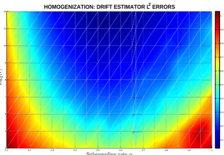
In Figure 3, we show an example of theL2_{error of the drift estimator with various}

scaling parameterand subsampling rateα. We see that the error is minimized around

α= 1/2as in Theorem 3.6.

3.3

The Diffusion Estimator

Just as in the case of the drift estimator, we define the diffusion estimator by the maxi-mum likelihood estimator (5), whereX is replaced by the discretized solution of (2a). More specifically, we define

˜

qN, ∆= 1

N∆

N−1

X

n=0

(xn+1−xn)2 (35)

wherex

n =xn∆is the discrete observation of the process generated by (2a) and∆is

0.1 0.2 0.3 0.4 0.5 0.6 0.7 0.8 0.9 1 4

5 6 7 8 9 10 11 12

Subsampling rateα

HOMOGENIZATION: DRIFT ESTIMATOR L2 ERRORS

−

log

2

(

ǫ

)

0.1 0.2 0.3 0.4 0.5 0.6 0.7 0.8 0.9 1

Figure 3: This is a colormap plot of theL2_{norm of the errors from the drift estimator} ˆ

aN,at different subsampling rates. Simulations are done through exact solution of the

multiscale OU system. Each path is subsampled withN = 1.5_{number of}

observa-tions, at time increment of∆ =α_{, withα}

∈[0.1,1]. We takefrom choices of2−4

to2−12_{. Each estimate is based on 100 paths. The initial condition is(x}

0, y0) = (0,0)

and the parameter values are a11 = a12 = a13 = a21 = a22 = −1, a14 = 1,

q1=q2= 2.

Theorem 3.8. Suppose that(x

t)t>0is the projection to thex-coordinate of a solution

of system(2)satisfying Assumptions 3.1. Letqˆbe the estimate we get by replacingX

in(5)byx_{, i.e.}

ˆ

q=

1

T

N−1

X

n=0

(xn+1−xn)2.

Then

E (ˆq−q˜)2=O

∆ +2+ 4 ∆2

whereq˜as defined in(18). Consequently, if∆ =α_{, fixT =N∆, andα}

∈(0,2), then

lim

→0E (ˆq−q˜) 2

= 0.

Furthermore,α= 4/3optimizes the error.

We first define

√

∆ηn=

Z (n+1)∆

n∆

dWt.

Proof. We now prove Theorem 3.8. Using the integral form of equation (23),

xn+1−xn =

Z (n+1)∆

n∆

p

˜

qdWs (36)

where

ˆ

R1, = ˜a

Z (n+1)∆

n∆

xsds

ˆ

R2, = a14a−221√q2

Z (n+1)∆

n∆

dVs

ˆ

R3, = (a12+a14)a−221

Z (n+1)∆

n∆

dy(s)

We rewrite line (36) as

Z (n+1)∆

n∆

p

˜

qdWs= p

˜

q∆ηn (37)

whereηnareN(0,1)random variables.

For∆andsufficiently small, by Cauchy-Schwarz inequality

E



 c

Z (n+1)∆

n∆

xsds

!2

 ≤ cE

Z (n+1)∆

n∆

(xs)2ds

Z (n+1)∆

n∆

ds

!

≤ c∆E

Z (n+1)∆

n∆

(x s)2ds

!

≤ c∆2E sup

n∆≤s≤(n+1)∆ (xs)2

!

= O(∆2)

Therefore,

E

( ˆR1,)2

=_O(∆2₎

By Itˆo isometry

E

( ˆR2,)2

=O(2∆)

Then we look atRˆ3,,

E

( ˆR3,)2

=2CE (yn+1−yn)2

By (28), we have

E

( ˆR3,)2

=_O(max(α,2)) (38)

We substitute(x

the estimator’s error as follows,

ˆ

q−q˜ = q˜(

1

N

N−1

X

n=0

ηn2−1)

+ 1

T

N−1

X n=0 3 X i=1 ˆ

R2i,

+ 2

T

N−1

X n=0 3 X i=1 ˆ Ri, p ˜

q∆ηn

+ 1

T

N−1

X

n=0



 X

i6=j

ˆ

Ri,Rˆj, 



= R

Then we bound the mean squared error using Cauchy-Schwarz inequality.

E

(ˆq−q˜)2

≤ Cq˜2E (1

N

N−1

X

n=0

ηn2−1)2 ! (39) + C 3 X i=1 E   1 T

N−1

X

n=0 ˆ

R2

i,

!2

 (40) + C 3 X i=1 E   1 T

N−1

X n=0 ˆ Ri, p ˜

q∆ηn

!2

 (41)

+ CX

i6=j

E





1

T

N−1

X

n=0

ˆ

Ri,⊗Rˆj,

!2

 (42)

By law of large numbers, line (39) is of order_O(∆). In line (40), fori∈ {1,2}, we have

E





1

T

N−1

X

n=0 ˆ

R2i,

!2

=

1

T2N

N−1

X

n=0

E

( ˆR2i,)2

.

Since_E( ˆR1,)2

=_O(∆2_{), we have}

E





1

T

N−1

X

n=0 ˆ

R21,

!2

=O N

2_(∆2₎2

=_O ∆2

;

sinceE

( ˆR2,)2

=_O(2_{∆), we have}

E





1

T

N−1

X

n=0 ˆ

R22,

!2

=O N2(∆2)2

The estimate is different forE



 _T1

N−1

X

n=0 ˆ

R23,

!2

. By (28), we have

E





1

T

N−1

X

n=0 ˆ

R23,

!2

 =

C4

T2 E



 N−1

X

n=0

yn+1−yn

2

!2



≤ C4_N

N−1

X

n=0

E

y

n+1−yn

4

= O

4+2 max(0,α−2) ∆2

= _O

max(4,2α) ∆2

Adding up all terms for line (40), we have,

3 X i=1 E   1 T

N−1

X

n=0 ˆ

R2i,

!2

=O

∆2+4+

max(4,2α) ∆2

. (43)

In line (41), fori_{∈ {}1,2_}, we have

E





1

T

N−1

X n=0 ˆ Ri, p ˜

q∆ηn

!2

≤CN2∆E

ˆ

Ri,ηn

2

=CNE

( ˆRi,)2

SinceE

( ˆR1,)2

=_O(∆2_{), we have}

E





1

T

N−1

X

n=0 ˆ

R1, p

˜

q∆ηn

!2

=O(N∆2) =O(∆);

sinceE

( ˆR2,)2

=_O(2_{∆), we have}

E





1

T

N−1

X

n=0 ˆ

R2, p

˜

q∆ηn

!2

=O(N 2∆) =O(2).

Again, it is different for _E



 _T1

N−1

X

n=0 ˆ

R3, p

˜

q∆ηn

!2

 due to correlation between

ˆ

R(3n,) and ηn. Using the expression from (37) by only considering the dominating

terms, we have

E





1

T

N−1

X

n=0 ˆ

R3, p

˜

q∆ηn

!2



= E 1

T

N−1

X

n=0 ˆ

R23, p

˜

q∆ηn

2 ! + E   1 T2 X

m6=n

ˆ

R(₃m_,)Rˆ₃(n_,)

Z (m+1)∆

m∆

p

˜

qdW s

Z (n+1)∆

By computing the order of the dominating terms and the martingale terms, when

m=n,

E _T1

N−1

X

n=0 ˆ

R23, p

˜

q∆ηn

2

!

= 1

T

N−1

X

n=0 ∆E

ˆ

R23,qη˜ 2n

= 1

TE( ˆR

2 3,η2n)

= _Omax(α,2)

and whenm < n,

E





1

T2

X

m6=n

ˆ

R(3m,)Rˆ

(n) 3,

Z (m+1)∆

m∆

p

˜

qdW s

Z (n+1)∆

n∆

p

˜

qdW s





≤ CN22E (yn+1−yn)(ym+1−ym )

×

Z (n+1)∆

n∆

dWs

Z (m+1)∆

m∆

dWs !

≤ CN22E (yn+1−yn)

Z (n+1)∆

n∆

dWs

× E (ym+1−ym )

Z (m+1)∆

m∆

dWs|Fm∆

!!

Using the expansion in (37), and using the dominating terms only,

E (ym+1−ym)

Z (n+1)∆

n∆

dWs|Fm∆

!

= E

(e−∆2 −_1)y m

+ 1

2

Z (m+1)∆

m∆

e−(m+1)∆2 −s_x sds

+ 1

Z (m+1)∆

m∆

e−(m+1)∆2 −s_dV s

!

Z (m+1)∆

m∆

dWs|Fm∆

!

= _O((e−∆2 −1))

Therefore, whenm < n, we have,

E





1

T2

X

m6=n

ˆ

R(₃m_,)Rˆ(₃n_,)

Z (m+1)∆

m∆

p

˜

qdW s

Z (n+1)∆

n∆

p

˜

qdW s





= O( 4 ∆2(e

−∆

2 −₁₎2₎

In the casem > n, the result is identical due to symmetry. Adding up all terms for line (41),

5

X

i=1

E





1

T

N−1

X

n=0 ˆ

Ri, p

˜

q∆ηn

!2



=_O∆ +2₊max(α,2)₊2 max(0,2−α) ₍₄₄₎

In line (42), we have

X

i6=j

E



 N−1

X

n=0 ˆ

Ri,Rˆj,

!2

≤NE (Ri,)2E(Rj,)2

Substituting in theL2_{norms of eachRˆ}

i,,i∈ {1,2,3}, we have for line (42),

X

i6=j

E



 N−1

X

n=0 ˆ

Ri,Rˆj,

!2



= _O∆22+ ∆max(α,2)+2+max(α,2) (45)

Aggregating bounds (43), (44) and (45) for equation lines from (39) to (42) respec-tively, we have

E (ˆq−q˜)2

= _O(∆)

+ O

∆2+4+

max(4,2α) ∆2

+ _O∆ +2+max(α,2)+2 max(0,2−α)

+ ∆22+ ∆max(α,2)+2+max(α,2)

It is clear that whenα <2,

E (ˆq−q˜)2

=_O(∆ +4−2α+2).

The error is minimized whenα= 4/3, which is of order

E (ˆq−q˜)2=O

43

.

It is easy to see whenα >2, the error explodes. This completes the proof.

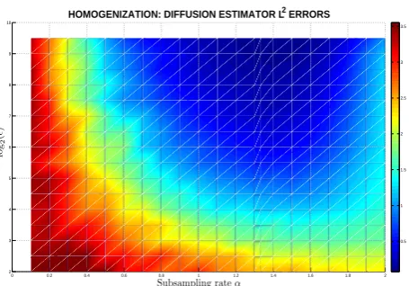
In Figure 4, we show an example of theL2 _{error of the diffusion parameter with}

0 0.2 0.4 0.6 0.8 1 1.2 1.4 1.6 1.8 2 2

3 4 5 6 7 8 9 10

HOMOGENIZATION: DIFFUSION ESTIMATOR L2 ERRORS

Subsampling rateα

−

log

2

(

ǫ

)

0.5 1 1.5 2 2.5 3 3.5

Figure 4: This is a colormap of theL2 _{norm of(ˆq}

−q˜)for differentandα. Each

path is generated over a fixed total time horizon ofT = 1, at a very fine resolution with

δ = 2−20_{, with available number of observationsN = 2}20_{. Each estimate is based}

on 100 paths. We test the scale parameterfrom2−2_to2−9.5_{, and test the diffusion}

estimator at a sequence of subsampling ratesαover each path at rates[0.1,2]. The system’s parameter values are a11 = a12 = a13 = a21 = a22 = −1, a14 = 1,

q1=q2= 2.

References

[1] A¨ıt-Sahalia, Y.; Mykland, P. A; Zhang, L. A Tale of Two Time Scales: Determin-ing Integrated Volatility With Noisy High-Frequency DataJournal of the

Ameri-can Statistical Association100(472)2005

[2] A¨ıt-Sahalia, Y.; Mykland, P. A; Zhang, L. How Often To Sample a Continuous-Time Process in the Presence of Market Microstructure NoiseThe Review of

Fi-nancial Studies182005

[3] Azencott, R.; Beri A.; Timofeyev, I. Adaptive sub-sampling for parametric esti-mation of gaussian diffusions.Journal of Statistical Physics139(6), 2010

[4] Azencott, R.; Beri A.; Timofeyev, I. Sub-sampling and parametric estimation for multiscale dynamics.SIAM Multiscale Model. Simul.2010

[5] Anderson, D. F.; Cracium, G.; Kurtz, T. Product-form Stationary Distributions for Deficiency Zero Chemical Reaction Networks.Bulletin of mathematical biology

72(8), 2010

[6] Bishwal, J.P.N. Parameter Estimation in Stochastic Differential Equations Springer-Verlag 2008

[7] Chen, X. Limit theorems for functionals of ergodic Markov Chains with general state space.Memoirs of the AMS129(664), 1999

[9] El Machkouri, M., Es-Sebaiy, K. and Ouknine, Y.. Least squares estimator for non-ergodic OrnsteinUhlenbeck processes driven by Gaussian processes.Journal

of the Korean Statistical Society45(3): pp 329–341, 2016.

[10] Graversen, S. E.; Peskir, G. Maximal Inequalities for the Ornstein-Uhlenbeck ProcessProceedings of the American Mathematical Society128(10), 2000

[11] Hall, P. and Heyde, C.C Martingale limit theory and its application. Academic Press, 1980.

[12] Isaacson, E.; Keller, H. B. Analysis of Numerical Methods Wiley & Sons. 1966.

[13] Ibragimov, I.; Hasminskii, R. Statistical estimation: Asymptotic theory. Springer, 1979.

[14] Kabanov, Y.; Pergamenschikov, S. Two-scale stochastic system: Asymptotic analysis and control. Springer, 2003.

[15] Kleptsyna, M. L. and Le Breton, A.. Statistical analysis of the fractional Orn-steinUhlenbeck type process.Statistical Inference for stochastic processes5(3): 229–248, 2002.

[16] Kutoyants, Y. A. Statistical inference for ergodic diffusion processes. Springer-Verlag, 2004.

[17] Liu, D.; Strong convergence of principle of averaging for multiscale stochastic dynamcial systemsComm. Math. Sci8(4)2010

[18] Maslowski, B. and Tudor, C.A.. Drift parameter estimation for infinite-dimensional fractional OrnsteinUhlenbeck process.Bulletin des Sciences

Math-matiques137(7): 880–901, 2013.

[19] Miao, W. Estimation of diffusion parameters in diffusion processes and their asymptotic normalityInternational Journal of Comtemporary Mathematical Sci-ence1(16)2006

[20] Olhede, S; Pavliotis, G. A. ; Sykulski, A. Multiscale Inference for High Fre-quency DataTech. Rep. 290 Department of Statistical Science, UCL2008

[21] Papavasiliou, A.; Pavlioitis, G. A.; Stuart, A. M. Maximum Likelihood Drift Es-timation for Multiscale DiffusionsStoch. Proc. Appl.119(10)2009

2003

[22] Pavliotis, G. A. ; Stuart, A. M. Multiscale Methods Averaging and Homogeniza-tion. Springer, 2008.

[23] Pavliotis, G. A. ; Stuart, A. M. Parameter Estimation for Multiscale DiffusionsJ.

Stat. Phys.1272007

[24] Prakasa Rao, B. L. S. Semimartingales and their statistical inference.Monograph