On the Regularity and Chaos of the Hydrogen Atom Subjected to External Fields

(1)

ISSN Online: 2167-9487 ISSN Print: 2167-9479

DOI: 10.4236/ijmnta.2018.72005 Jun. 29, 2018 56 Int. J. Modern Nonlinear Theory and Application

On the Regularity and Chaos of the Hydrogen

Atom Subjected to External Fields

Jaouad Kharbach

1

, Walid Chatar

1

, Mohamed Benkhali

1

, Abdellah Rezzouk

1

,

Mohammed Ouazzani-Jamil

2

1_{Laboratoire de Physique du Solide, Faculté des Sciences Dhar El Mahraz, Université Sidi Mohamed Ben Abdellah, Fès-Atlas,} Morocco

2_{Université Privée de Fès, Laboratoire Systèmes et Environnements Durables, Lot. Quaraouiyine Route Ain Chkef, Fès, Morocco}

Abstract

In this paper, the integrable classical case of the Hydrogen atom subjected to three static external fields is investigated. The structuring and evolution of the real phase space are explored. The bifurcation diagram is found and the bi-furcations of solutions are discussed. The periodic solutions and their asso-ciated periods for singular common-level sets of the first integrals of motion are explicitly described. Numerical investigations are performed for the in-tegrable case by means of Poincaré surfaces of section and comparing them with nearby living nonintegrable solutions, all generic bifurcations that change the structure of the phase space are illustrated; the problem can exhibit regularity-chaos transition over a range of control parameters of system.

Keywords

Hydrogen Atom, Zeeman Effect, Stark Effect, Van Der Waals Interaction, Hamiltonian System, Integrability, Bifurcation, Chaos, Poincaré Surfaces of Section

1. Introduction

Most natural phenomena are generally governed by nonlinear differential equa-tions, for these problems, we must use different mathematical approaches and computational methods to simplify these systems and to study their integrable like lie algebra, the Painlevé criterion, the Ziglin criterion, the Liouville theorem and the Poincaré sections, because physically integrable systems are rare.

The study of the Hydrogen atom has been recently the focus of many works

[1]-[10]. Its great importance lies in its fields of implications in different

How to cite this paper: Kharbach, J., Cha-tar, W., Benkhali, M., Rezzouk, A. and Ouazzani-Jamil, M. (2018) On the Regular-ity and Chaos of the Hydrogen Atom Sub-jected to External Fields. International Journal of Modern Nonlinear Theory and Application, 7, 56-76.

https://doi.org/10.4236/ijmnta.2018.72005

Received: April 13, 2018 Accepted: June 26, 2018 Published: June 29, 2018 Copyright © 2018 by authors and Scientific Research Publishing Inc. This work is licensed under the Creative Commons Attribution International License (CC BY 4.0).

http://creativecommons.org/licenses/by/4.0/

(2)

DOI:10.4236/ijmnta.2018.72005 57 Int. J. Modern Nonlinear Theory and Application branches of physics: solid state physics [11], spectroscopy [12], plasmas physics

[13], molecular physics [14], astrophysics [15].

The Hydrogen atom is a simple but very complicated system when introduc-ing external fields. The Hydrogen atom in a static magnetic field is a simple sys-tem that can be studied experimentally and theoretically, its dynamics in such a field has been a source of many interesting results in atomic physics over the past two decades [16] [17]. It proves to be a prototype of quantum systems whose classical behavior can show chaotic dynamics [18] [19]. Concrete systems are often modeled using systems with natural parameters. The regularity of the behavior of the system is observed for certain values of the parameters, but usually the behavior of the dynamical system becomes unpredictable.

The Hydrogen atom under the effect of external fields is a complicated, non-separable problem and generally displays chaotic behavior for some com-binations of the appropriate parameters. The chaotic appearance results from the fact that, for certain initial conditions, the behavior of the dynamic system becomes unpredictable [20]. The chaos is identified by a high sensitivity to the initial conditions and by the variation of the control parameters of the system. Indeed, a system with n degrees of freedom is regular if there are n independent constants of motion [21]. Most problems involving atoms in external fields are very difficult to study analytically and solutions are difficult to obtain. However, for combinations of appropriate parameters, one can find exact solutions.

The isotropic nonrelativistic Hydrogen atom subjected to three static external fields: a magnetic field, an electric field, and a van der Waals interaction. The Hamiltonien (in units such that me= = = e a0 =1) can be written as:

(

) (

)

2 2 2 2 2 2 2

1 1

2

H p x y z x y z

r α λ γ β

= − + + + + + + ₍₁₎

where _r2₌_x2₊_y2₊_z2_, 2 2 2 2

x y z

p = p +p +p _{, and}

α λ γ

, , _and

β

_{are control} parameters representing the magnitude of the applied external fields: α is a con-stant; γ, measured in units of magnetic field 5

0 2.35 10 T

B = × , controls the qua-dratic Zeeman effect; β, measured in units of electric field 11

0 5.14 10 V cm

F = × ,

controls the Stark effect; and the a-dimensional number λ controls the anhar-monicity associated to the van der Waals interaction [10] [11] [12]. This com-bined potential is very interesting because of its similarity to the fields seen by an ion confined in a Paul trap [13].

(3)

com-DOI: 10.4236/ijmnta.2018.72005 58 Int. J. Modern Nonlinear Theory and Application mon-level sets of the constants of motion. In section 5 we also investigate nu-merically via Poincaré surfaces of section, the structure and evolution of the phase space for the integrable case, comparing them with nearby living nonin-tegrable solutions, the problem can exhibit regularity-chaos transition over a range of system control parameters. Finally, Section 6 contains our conclusions.

2. Equations of Motion

The regularized Hamiltonian is obtained by transforming Equation (1) to semi-parabolic coordinates and the corresponding momenta, namely,

( )

2 2 cos , sin , , 2 x uv y uv u v z ϕ ϕ = = − =

( )

2 2 2 2 2 2

cos cos cos sin

,

sin sin sin cos

,

.

x u v

y u v

z u v

v v u

p p p p

uv

u v u v u v

v v u

p p p p

uv

u v u v u v

u u v

p p p

u v u v u v

ϕ

ϕ ϕ ϕ ϕ

= + − + + + = + + + + + = − + + + (2)

Note that the equations of motion associated with the Hamiltonian (1) have a collision singularity at r=0, which can be removed with the following change in the independent variable

(

2 2

)

d

dτt r u v= = +

After such transformation, the regularized Hamiltonian reads

( )

(

)

(

)

(

)

(

)

(

)

2 2

2 2 2 2 6 6

2 2

2

4 4 4 2 2 4

1 1 1

, 2

2 2 4

2 4

u v

p

u v p p H u v u v

u v

u v u v

H

u v

ϕ αλ

β _{α γ} αλ

  = = + + _ + _− + + +     + − +_ + − _ +    (3)

In this equation, pϕ is a conserved quantity, represents the value of the cy-clic integral associated to the cycy-clic coordinate φ, and we put pϕ =l, with l a constant.

The difference between the Hamiltonian (3) and the Hamiltonian of an ion in

a Paul trap is that the total pseudo-energy H is equal to2, that of a trapped ion

is −2 (for details, see Ref. [11]).

The equations of motion associated with H u

( )

,v in the new time τ are,

therefore,

(

)

(

)

2 2 2

3 5 3 2 4

3

2 2 2

3 5 2 3 4

3

,

2 2 6 4 2 ,

4 4

,

2 2 6 4 2 .

4 4 u u v v u p l

p hu u u u v uv

u v p

l

p hu v v u v u v

v

αλ αλ

β α γ

αλ αλ

β α γ

=   = − − + −_ + − _ +   =   = + − + −_ + − _ +       (4)

the dot denotes derivative with respect to τ.

(4)

DOI:10.4236/ijmnta.2018.72005 59 Int. J. Modern Nonlinear Theory and Application

the real three dimensional system after ignoring the cyclic integral associated to

the cyclic coordinate φ, pϕ = =l 0.

The study of the dynamics for Hydrogen atom subjected to external fields is easier to process in two-dimensional standardized version than a three-dimensional; and by removing the Coulomb singularity from the original dynamic system, the regularization procedure facilitates the numerical work. Another practical aspect is that the regular 2D Hamiltonian is equivalent to the motion of two coupled anharmonic oscillators with pseudo-energy is equal to 2, a system for which there are effective tools to make the problem easily exploita-ble.

3. The Phase Space Topology

The two dimensional regularized Hamiltonian (3) is separable if the relation (5) is verified

2

0 2 1

4

αλ γ

α γ λ

α

+ − = ⇔ = ± + ₍₅₎

in this case the second integral of motion reads

(

)

(

)

(

)

(

)

(

)

2 2 2 2 6 2 6 2 2 4 2 4 2

2 2

2 2 2 2

2

2 2

v u

u p v p v u u v v v u u v

F f

u v

u v u v

α γ

β

− + − + +

= = + −

+

+ + (6)

(

)

2 2 2

2 2

1 2

2

x x z z

F f zp xp p x z x

x z

β α γ

= = − + − − + −

+ (7)

It is easy to verify that Equation (2) becomes

2 2 , , 2 x uv u v z = − =

( )

1 2

2 2 2 2 2 2

1 2

2 2 2 2 2 2

,

. x

z

v v u

p g u g v

u v u v u v

u u v

p g u g v

u v u v u v

= + + + + = − + + + (8) where

( )

2 2 4

(

)

6

1 u 2 2 ₂

g u =p = _ − +f hu −βu − α γ+ u _

  (9)

( )

2 2 4

(

)

6

2 v 2 ₂

g v = p = _f hv+ +β v − α γ+ v _

  (10)

in these conditions, the equations of motion are

( )

1 2 , . u v

u p g u

v p g v

= = ±



 (11)

H h= _and F f= _{are the first integrals of motion, functions of}

(

u v p p, , ,u v

)

which are constant along the solutions of Equation (11). The sys-tem is called (meromorphically) Liouville integrable or completely integrable.

3.1. The Bifurcation Diagrams and the Admissible Region

(5)

DOI: 10.4236/ijmnta.2018.72005 60 Int. J. Modern Nonlinear Theory and Application

and a detailed description of the real phase space topology i.e. the topology of

the real level sets for all generic constants h and f:

(

)

{

_{, , ,} 4_: _,

}

4

u v

A_ = u v p p ∈ H h F f= = ⊂

For doing that we find first the bifurcation diagram B of the problem (12), i.e. the set of critical values of the energy-momentum mapping

(

u v p p, , ,u v

)

→

(

H F,

)

It appears, according to several works carried out in this sense (for details, see

Ref. [22]-[27]), that the bifurcation diagram B is exactly the discriminant locus

of the polynomials g u1

( )

and g v2

( )

whose coefficients are functions in h f,

and the parameters of the system

(

α β γ

, ,

)

.

1 2

B B B= _

(

)

(

( )

)

{

}

(

)

(

( )

)

{

}

5

1 5

2

, , , , : 0

B h f discr g u

h f discr g v

α β γ α β γ

= ∈ =

∈ =



 

It is convenient to consider separately, for some values of the constants α, β

and γ, two cases

λ

≥2 and

λ

<2, because they generate different structures

of the topology of the real level sets A and the corresponding Poincaré map.

3.1.1. For the Case

λ

≥2

(

)

(

)

2 2 3 2

1

2 2 3 2

2

1348 2

, : 2, 1 45 675 3375

675 15 675

2 2

, : 0, 1 45 675 3375

675 15 675 h

B h f f f h h h

h

B h f f f h h h

 

=_ ∈ = = − ± + + + _⊂

 

−

 

=_ ∈ = = − ± + + + _⊂

 

 

(14) The set

{

_3_\_B

}

_

{

_λ _≥₂

}

_{consists of 10 connected components (as it is} shown in Figure 1). Thus, in each connected component of the set A B\ the level set A_ has the same topological type, and this latter may be changed only if

(

h f,

)

passes through B_

{

λ ≥2

}

_.

Theorem 1. The set

{

_3_\_B

}

_

{

_λ _≥₂

}

_{consists of ten connected}

compo-nents. The sections of these components with the plane

{

λ

=const.

}

are shown on Figure 1. If

(

_{h f}_{, ,}

_λ

)

_∈_3_\_B_{the topological type of} _A

 is (diffeomorphic

to) a two-dimensional tori T, to a disjoint union of two-dimensional two-tori 2T,

or it is the empty set ϕ as it is shown in Table1.

Proof. Consider the complexified system

(

)

{

_{, , , ,} 5_: _., _., 2 2 2_, ₀

}

x z

A⊄= x z p p r ∈⊄ H h const F f const r= = = = =x +z r≠

consider also the hyperelliptic curves

{

2

( )

}

1: ω1 g u1

Γ = _and

{

2

( )

}

2: ω2 g v2

Γ =

and the corresponding Riemann surfaces R1 and R2 of the same genus

1 2 2

j = j = _{. We obtain the explicit solutions of the initial problem (11) by}

(6)

[image:6.595.211.537.87.504.2]

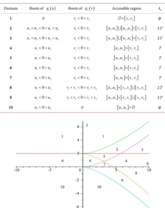
Table 1. The Topological type of A_, and the admissible set for

(

_{h f}_,

)

_∈_2_\_B_.

Domain Roots of g u1

( )

Roots of g v2

( )

Accessible region A

1 0 v1< <0 v2 ∅×

[

v v1, 2

]

∅

2 u u1< 2< <0 u u3< 4 v1< <0 v2

[

u u1, 2

] [

 u u3, 4

] [

×v v1, 2

]

2T

3 u u1< 2< <0 u u3< 4 v1< <0 v2

[

u u1, 2

] [

 u u3, 4

] [

×v v1, 2

]

2T

4 u1< <0 u2 v1< <0 v2

[

u u1, 2

] [

×v v1, 2

]

T

5 u1< <0 u2 v1< <0 v2

[

u u1, 2

] [

×v v1, 2

]

T

6 u1< <0 u2 v1< <0 v2

[

u u1, 2

] [

×v v1, 2

]

T

7 u1< <0 u2 v1< <0 v2

[

u u1, 2

] [

×v v1, 2

]

T

8 u1< <0 u2 v v1< < < <2 0 v v3 4

[

u u1, 2

] [

×v v1, 2

] [

 v v3, 4

]

2T

9 u1< <0 u2 v v1< < < <2 0 v v3 4

[

u u1, 2

] [

×v v1, 2

] [

 v v3, 4

]

2T

10 u1< <0 u2 0

[

u u1, 2

]

×∅ ∅

Figure 1. Bifurcation diagram B

{

λ=const.

}

and the numbering of domains for λ ≥2_.

Thus x z p p, , ,x z can be expressed in terms of hyperelliptic functions living in the Jacobi variety Γ = Γ ⊗ Γ1 2 (where ⊗ is the symmetric product). These

functions however are not single valued as can be seen from formulae (8) and (11).

Indeed, to each point on the symmetric product Γ ⊗ Γ1 2 there correspond

two values of

(

x z p p, , ,x z

)

. Thus we define the natural projection

1 2

:A

π

⊄→ Γ ⊗Γ

corresponding to the involution i

(

) (

)

: , , ,x z , , x, z

i x z p p → x z p− −p

[image:6.595.208.538.94.494.2]

(7)

conju-DOI: 10.4236/ijmnta.2018.72005 62 Int. J. Modern Nonlinear Theory and Application gation on A⊄:

(

) (

)

: , , ,x z p px z x z p p, , ,x z

η

→ (15)

Consider also the natural projection ξ on the Riemann surface R R= 1⊗R2

given in u, v coordinates by:

( ) (

)

: ,u v u v,

ξ

→

It induces an involution on the Jacobi variety and hence on A⊄ by the natu-ral projection π. Formulae (6) and (7) imply that this involution ξ coincides with the complex conjugation (15) on A⊄ the upshot is that in order to describe

A_ it is enough to study the projection:

( )

1 2

:A Jac R

π

⊄→ = Γ ⊗ Γ

Definition. A connected component of the set of fixed points of η on the curves

1

Γ _and Γ₂_{is called an oval.}

To determine the ovals of Γ1 and Γ2 it suffices to study the real roots of

the polynomials g u1

( )

and g v2

( )

for different values of h and f as shown in Table 1. Using the formulae (8) and the condition that

(

_{, , ,}

)

4

x z

x z p p ∈_ _{, we}

find exactly two admissible ovals whose projections on the u-plane and the

v-plane are given by ∆1 and ∆2. The product of the admissible ovals in

1 2

Γ ⊗ Γ _{and the projection}_π_of A_ such as, 1

(

)

1 2 1 2

A ₌

π

− _Γ _⊗_{Γ = ∆ × ∆}

 ,

gives:

3.1.2. For the Case

λ

<2

(

)

2 2 3 2

1 , : 2, 484_{243 9 243}h 2 1 27 243 729

B′ =_ h f ∈ f = f = + ± − h+ h − h _⊂

   

(

)

2 2 3 2

2 , : 0, _{243 9 243}2 h 2 1 27 243 729

B′ =_ h f ∈ f = f = − + ± − h+ h − h _⊂

   

Theorem 2. The set

{

_3_\_B_′

}

_

{

_λ _<₂

}

_{consists of ten connected components}_.

The sections of these components with the plane

{

λ

=const.

}

are shown on Figure 2. If

(

_{h f}_{, ,}

_λ

)

_∈_3_\_B_′_{The topological type of} _A

 is (

diffeomor-phic to) a two-dimensional tori T, to a disjoint union of cylinders C, or it is the real planes _2_{as it is shown in}_{Table 2}_.

3.2. Topology of Singular Level Sets and Bifurcations of Liouville

Tori

Suppose now that the constants h, f are changed in such a way that

(

h f,

)

passes through the bifurcation diagram B. Then the topological type of A may change and the bifurcation of Liouville tori takes place.

For the first case

λ

≥2_{, According}_to _{Fomenko surgery on Liouville tori}

[29], we can have in our case three types of bifurcation of the level set A_ (see

Table 3). To prove that, it suffices to look at the bifurcations of roots of the polynomials g u1

( )

and g v2

( )

. The correspondence between bifurcation of

(8)

Figure 2. Bifurcation diagram B′

{

λ=const.

}

and the numbering of domains for λ <2.

Figure 3. Correspondence between bifurcation sets for

(

h f,

)

∈B and bifurcation of invariant Liouville tori, where

(

S S∧

)

_{is a union of two} circles having exactly one common point.

Table 2. The topological type of A, and the admissible set for

(

h f,

)

∈2\B′.

Domain Accessible region A

1’ ]−∞,u1] [ u2,+∞ × −∞ +∞[ ] , [ 22

2’ ]−∞,u1] [ u2,+∞ × −∞ +∞[ ] , [ 22

3’ ]−∞,u1] [ u2,+∞ × −∞[ ] ,v1] [ v v2, 3] [ v4,+∞[ 2C+42

[image:8.595.232.514.70.248.2] [image:8.595.234.514.302.531.2]

(9)

DOI: 10.4236/ijmnta.2018.72005 64 Int. J. Modern Nonlinear Theory and Application Continued

5’ ]−∞,u1] [u u2, 3] [u4,+∞ × −∞ +∞[ ] , [ C+22

6’ ]−∞ +∞ × −∞ +∞, [ ] , [ _2

7’ ]−∞ +∞ × −∞, [ ] ,v1] [v v2, 3] [ v4,+∞[ C+22

8’ ]−∞,u1] [u u2, 3] [ u4,+∞ × −∞[ ] ,v1] [ v2,+∞[ 2C+42

9’ ]−∞ +∞ × −∞, [ ] ,v1] [ v2,+∞[ 22

[image:9.595.206.540.82.219.2]

10’ ]−∞ +∞ × −∞, [ ] ,v1] [ v2,+∞[ 22

Table 3. Generic bifurcations of the level set A.

6→1 6→10

2→1 9→10

2→5,9→10

3→4,8→4

T→φ 2T→φ 2T→T

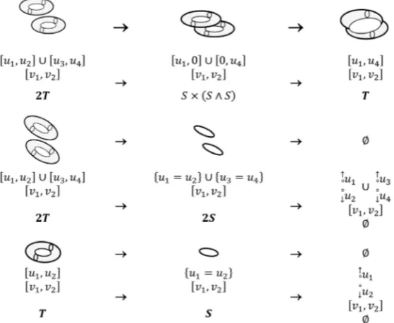
As shown in Figure 3, three types of bifurcations of (surgery on) Liouville tori take place:

1) Bifurcation T→ → ∅S : The two dimensional tori T is contracted to the cir-cle S corresponding to the periodic solution, and then vanishes.

2) Bifurcation 2T→ ×S S S

(

∧

)

→T: The two dimensional two tori 2T merge into two dimensional tori T by passing through the complex S×

(

S S∧

)

where

(

S S∧

)

is a union of two circles having exactly one common point. 3) Bifurcation 2T→2S→ ∅_{: The two dimensional two tori 2}T_{are contracted}

to two circles 2S corresponding to two periodic solutions, and then vanishes. For the second case λ <2_{, The Fomenko classification of bifurcation of} Liouville tori [29] cannot be applied as its invariant level sets contain a non-compact component (cylinder C or plane _2_{). Thus, we can have the type} of bifurcation of the level set A passing from domain i to domain j in Table 4.

To prove that, it suffices to look at the bifurcation of roots of the polynomials

( )

1

g u and g v2

( )

as shown in Figure 4.

4. Periodic Solutions

4.1. For the Case

λ ≥

2

When the bifurcation of Liouville tori takes place, the level set A_ becomes completely degenerate. Then we can have exceptional families of periodic solu-tions. It is seen from Table 5, that if

(

h f,

)

is on the smooth curves C C0

( )

0′

or C C1

( )

1′ (see Figure 5), A contains a isolated circles S and 2S, respec-tively which are periodic solutions. Consider now a fixed periodic solution be-longing to the curve C0. The parameter v takes values in the admissible interval

[

v v1, 2

]

and u u u= 1= 2 is equal to the double root of the polynomial g u1

( )

(10)

[image:10.595.212.533.111.674.2]

DOI:10.4236/ijmnta.2018.72005 65 Int. J. Modern Nonlinear Theory and Application Then we obtain from Equation (8) the following parameterization of fixed pe-riodic solution:

(11)

[image:11.595.233.517.76.271.2]

[image:11.595.208.541.325.378.2]

Figure 5. Topological type of A for

(

h f,

)

∈B and λ ≥2.

Table 4. Generic bifurcations of the level set A.

4′→3′

4′→8′

4′→5′

4′→7′

3′→2′

8′→9′

5′→6′

7′→6′

2 2

4 4 2 4

T+ C+  → C+  _T₊₄_C₊₄_2_{→ +}_C ₂_2 ₂_C₊₄_2_→₂_2 _C₊₂_2_→₂_2

Table 5.Topological type of A_ for

(

h f,

)

∈B.

Curves Accessible region A

0

C {u u1= 2}×[v v1, 2] S

1

C {u1=u2} { u3=u4}×[v v1, 2] 2S

0

C′ [u u₁, ₂] {× v v₁= ₂_} S

1

C′ _[u u₁, ₂_{] {}× v v₁= ₂_{} {} v₃=v₄_} 2S

( )

2

0 0

and 2

x

z p x

v g v

z p

v =  =



 

 ₌− 

= ±

 

 _

(16)

to derive the differential equation satisfied by v, we use

d d_τv p= v we obtain from (10)

( )

2

dv _d

g v = ± τ

[image:11.595.208.542.401.712.2]

(12)

DOI:10.4236/ijmnta.2018.72005 67 Int. J. Modern Nonlinear Theory and Application On the curve C0, the second integral of motion f is equal to 2, as well as the

characteristic polynomial

( )

2

(

2 4 6

)

2 v 2 2 5

g v =p = +hv +v − v _{depends only on}_h_. Taking this variable change:

2 d _d

2 R

R v v

R

= ⇒ =

(

3 2

)

( )

2

d d

d

2 2

2 2 2 5

R R

P R

R hR R R

τ = ± = ±

+ − + (17)

the polynomial P R2

( )

has four distinct roots

0 0

R = ,

1 3 1 1 3 1 2 ₁ 15 30 15 h D R D  ₊     

= + + , R2=a ib0+ 0 et R3=a ib0− 0

where 1 3 0 1 3 1 1 15 60 15 h D a D  ₊    − _ _ = − + , 1 3 0 1 3 1 3 15 2 60 h D b D   ₊    ₋ _ _   = −       3 2

180 5408 60 60 3 540 8124

D= h+ + − h − h + h+

By an inversion of the elliptic integral Equation (17), one explicitly obtains the expression the periodic solution v

( )

τ :

(

)(

)

0 0

0 1 2 3

1 d d 2 2 R R R

R R R R R R R R τ

τ =

− − − −

∫



(18)

(

)

1

0 cos , 0

n Cn k

τ

₌ −

ϕ

where

(

)

2 2

1 0 0

0 0 0 0 0 0 1 _, 4 2 2

R A B

n k

A B A B

− −

= = _, 2 2 2 2 2 2

0 1 0, 0 0 0

A =R +a B =b +a

(

)

(

)

1

0 0

cos , ,

Cn−

ϕ

k ₌F

ϕ

k _{being the incomplete elliptic integral of first kind.} The expression of periodic solution v

( )

τ

is given by solving the Jacobi inver-sion problem:

( )

(

)

{

}

(

) (

)

(

)

1 0 0 0

2 0 0 0 0 0 0

2 2 1

d d

2 2 R B Cn t A B v

t v

g v A B A B Cn t A B

τ

τ= = ⇒ τ = ± −

+ + −

∫

The period Tv associated with the solution v t

( )

is obtained by calculating the elliptic integral Equation (17) over the totality of the admissible oval for v:

( )

₍

₎

1

0 3 2

2

d

1 d 2

d

2 2 2 2 ₂ ₅

R y

v _R

p R

T

P R _R _hR _R _R

τ

= = =

+ − +

∫



It’s sufficient to replace in Equation (18) the upper bound in the integral by

1

(13)

de-DOI: 10.4236/ijmnta.2018.72005 68 Int. J. Modern Nonlinear Theory and Application pendent only on the energy h:

( )

1

(

)

(

)

0 0 0 0

2 1, 2 π,

v

T h ₌ n Cn− ₋ k ₌ n F k

where 1

(

)

(

)

0 0

1, π,

Cn− ₋ k ₌F k _{is the complete elliptic integral of the first kind.} In the same way, for the periodic solution on the curve C1 the parameter v

takes values in the admissible oval

[

v v1, 2

]

, the double roots of the polynomial

( )

1

g u are equal to u u1= 2= −m and u3=u4=m (see Table 5).

The values of the first integrals H and F on the curve C1 are related by

2 3

1348 _{2 1 45 675 3375}

675 15 675 h

f = − + + h+ h + h

From Equation (8) we obtain the following parameterization of fixed periodic solution

( )

2 2 2 2 2 2 2 2 and 2 x z m

x mv p g v

m v

m v _v

z _p _{g v}

m v  = ±  _ = ±   +  ₌ −    _{= ±}  __ ₊ (19)

( )

{

(

)

}

(

) (

)

(

)

1 1 1 1

1 1 1 1 1 1

2 2 1

2 2

R B Cn t A B

v t

A B A B Cn t A B

− = ±

+ + −

The period of v t

( )

is

( )

1

(

)

(

)

1 1 1 1

2 1, 2 π,

v

T h ₌ n Cn− ₋ k ₌ n F k

where

(

)

2

1 1 1 2 2 2 2

1 1 1 1 1 1

1 1 1 1

2 2

1 1

1 _, _, _,

4

2 ,

2

R A B

n k A R a B b a

A B A B − − = = = + = + 1 1 3 3

0 1 1 1 1

3 3

1 15 1 1 15 1

0, 1 , 2 ,

15 30

h h

R R C a C

C C  ₊  ₋  ₊      = = _ + + _ = _ + − _     1 3 1 1 3

3 15 _{1 ,}

30 h b C C  ₊    = _ − _  

(

)

(

)

(

)

3 3 2 3

675 1 15 1

911249 20503080 307546200 1537731000 911250 15 1

C h

h h h h

= + +

+ + + + + +

From Equation (19), the Cartesian equation for this periodic solution in the

( )

x z, plan is

( )

2 2₂

2 2

m x

z x

m

= −

4.2. For the Case

λ <

2

(14)

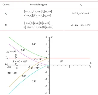
DOI:10.4236/ijmnta.2018.72005 69 Int. J. Modern Nonlinear Theory and Application values of the second integral of motion f is equal to 2 (f is equal to 2) (see Figure 6), A contains a circles S which correspond to a periodic solutions. On the curve L f0

(

=2

)

the periodic solution v t

( )

is given by

( )

{

(

)

}

(

) (

)

(

)

0 0 0

0 0

1

0 0 0 0

2 2 1

2 2 R B Cn t A B v t

A B A B Cn t A B

′ ′ ′ −

= ±

′+ ′ + ′− ′ ′ ′

The associated period is

( )

2 0 1

(

1, 0

)

2 0

(

π, 0

)

v

T h ₌ n Cn_′ − ₋ k_′ ₌ n F_′ k_′ where

(

0 0

)

0 0

0 0 2 2

1 2 2 2 2 2 2

0 1 0 0 0

0

0 0

0

1 _, _, _, _, _0,

4 2 2

R A B

n k A R a B b a R

A B A B ′ ′ − ′= ′= − ′ = + ′ ′ = ′ + ′ = ′ ′ ′ ′

1 1 1

3 3 3

0 0 0

1 1 0 1 0 1

3 3 3

0 0 0

1 1 1

2 2

1 1 3

9 _, 9 _, 9 _,

18 9 36 9 2 18

h h h

D D D

R a b

D D D

   ₋   ₋   ₋    ₋          _  _ = − − = + − = +       3 2

0 108 1952 36 36 3 324 2940

[image:14.595.202.538.63.725.2]

D = h− + h − h − h+

Table 6.Topological type of A for

(

h f,

)

∈B′.

Curves Accessible region A

0

L

]

{ }

[

]

11

] [

22 33

] [

44

[

, ,

, , ,

u u u u

v v v v

−∞ = +∞

× −∞ +∞

 

2

2 v 2 4

S+  + C+ 

0

L′

]

] [

[

]

11

]

{223 3} 4

[

4

[

,

, ,

u u u u v v v v

−∞ +∞

× −∞ = +∞  

 

2

2 u 2 4

S+  + C+ 

[image:14.595.211.539.384.702.2]

(15)

5. Numerical Investigation

By making use a set of software routines, implemented in Maple, for plotting 2D projections of Poincaré surfaces of section, method introduced by Poincaré and extended by Hénon [30], we give numerical illustrations of the real phase space topology studied in Section 3. For fixed values of constants h f, , ,α λ and

,

β γ

vary, the Liouville tori contained in the level set

{

H h F f= , =

}

change their topological type, while preserving the integrable behavior of the problem. However, with increasing control parameter associated with magnetic field, the random scattering of points in the sections shows that the system has carried out a transition from regularity through a quasi-regularity to chaotical dynamics.

The Poincaré surfaces of section are plotted in the plane

(

q p1, 1

)

=

(

u p, u

)

.

5.1. Regularity-Chaos Transition

Figures 7(a)-(h) represent Poincaré surfaces of section for

β

=2_{(electric field)} and values of γ (magnetic field) near the integrable case

γ

=4_{(from left to} right), where for different values of h and f on the bifurcation diagram B the system is totally regular, the topological type of A_ is diffeomorphic to a two-dimensional tori T, or a disjoint union of two-dimensional two-tori 2T. When the magnetic field increases for

γ

=4_to

γ

=4.5_{, the corresponding} Poincaré surfaces of section show that the system go through a transition from regularity to chaotical dynamics. At

γ

=5_{(high magnetic field), all Poincaré} surfaces of section show a strong irregular motion, the dynamic is totally cha-otic.

Figures 8(a)-(h) show the Poincaré surfaces of section for

β

=0_{(no electric} field) and

γ

=4_{, the system still has a regular motion, so we can say that the} electric field is not responsible for the chaotic behavior of the system, on the other hand only the variation of the intensity of the magnetic field changes the behavior of the system from regularity to chaotically dynamics.

5.2. Bifurcations of Liouville Tori

Figure 9(a) represents the Poincaré surfaces of section for the bifurcation 2T→2S→

φ

_{, when the system evolves from domain 2 to domain 1 on the} bi-furcation diagram where the values of the integrals of motion are h=4.685

(16)

(17)

[image:17.595.226.530.64.166.2]

DOI: 10.4236/ijmnta.2018.72005 72 Int. J. Modern Nonlinear Theory and Application Figure 7.Poincaré surfaces of section for

(

_{h f}_,

)

_∈_2_\_B_and _λ _≥₂_{. The three}

sur-faces (from left to right) correspond to β =2 (electric field) and γ =4, 4.5,5 (mag-netic field). (a) Domain 2 (h=7.477,f =3.936)A_≈2T ; (b) Domain 3

(h=8.873,f =3.096)A_≈2T_{; (c) Domain 4} (h=7.155,f =1.112)A_≈T

; (d) Domain 5

(h=2.269,f =1.583)A_≈T_{; (e) Domain 6}(h=0.819,f =1.011)A_≈T

; (f) Domain 7

[image:17.595.222.525.291.454.2]

(h=3.021,f =0.305)A_≈T_{; (g) Domain 8}(h=7.477,f = −1.376)A_≈2T_{; (h) Domain} 9 (h=7.477,f = −2.553)A_≈2T.

Figure 8. Poincaré surfaces of section for

(

_{h f}_,

)

_∈_2_\_B_and _λ _≥₂_{. The} surfaces correspond to β =0 (no electric field) and γ =4 (magnetic field). (a) Domain 2; (b) Domain 3; (c) Domain 4; (d) Domain 5; (e) Domain 6; (f) Domain 7; (g) Domain 8; (h) Domain 9.

Figure 9.Poincaré surfaces of section on the bifurcation diagram for

(

h f,

)

∈B

[image:17.595.226.524.526.687.2]

(18)

DOI:10.4236/ijmnta.2018.72005 73 Int. J. Modern Nonlinear Theory and Application domain 8 to domain 4 where h=7.155 and f = −0.738_{(black), 0 (blue),} 1.112 (orange). Figures 9(e) represents the bifurcation 2T → ×S S S

(

∧

)

→T, from domain 9 to domain 7 where h=3.021 and f = −0.569_(black),_{0 (red),} 0.305 (blue). Figures 9(f) represents the bifurcation 2T→ ×S S S

(

∧

)

→T, from domain 2 to domain 5 where h=3.88 and f =1.616_{(black), 2 (red),} 2.625 (blue). Figures 9(g) represents the bifurcation T→ →S

φ

_{, from domain} 6 to domain 1 where h= −4.067 and f =1_{(black), 1.437 (blue), 1.891 (red),} 2 (black dot). Figures 9(h) represents the bifurcation T → →S

φ

_{, from} do-main 6 to dodo-main 10 where the values of integrals of motion are h= −4.067

and f =1_{(black), 0.5 (blue), 0.2 (red), 0 (black dot). The black dots} corres-pond to the periodic solutions in the form of a isolated circles.

For the case

λ

<2, the invariant level sets contain a non-compact compo-nent (cylinder C or plane _2_{), only in the domain 4’ on the bifurcation}

dia-gram B′_{we find a single tori.}

Figure 10(a) shows the Poincaré sections for λ = ± 3 and for a values of the integrals of motion h= −7.879_and f =0.825_{(black), 1.122 (red), 1.758} (blue) corresponding to a point of domain 4’ on the bifurcation diagram B’, where A is a two-dimensional tori T.

Figure 10(b)shows the Poincaré sections for λ = ± 3 corresponding to the bifurcation ₄ ₄ 2 ₂ ₂ ₄ 2 ₂ ₄ 2

u

T+ C+  → +S  + C+  → C+  from domain 4’ to domain 3’ on the bifurcation diagram B’ , where the values of the integrals of motion are h= −7.879_and f =1.9_{(black), 2 (black dot), this black dot} con-cerns the periodic solution in the form of a circle.

6. Conclusion

In this paper, we have studied the classical dynamics of the Hydrogen atom in the generalized van der Waals potential subjected to external parallel magnetic and electric fields. By making use of some reductions, the regularized Hamil-tonian of the system is described by a two-degree of freedom dependent on certain control parameters. The converted system is equivalent to the motion of

[image:18.595.241.507.554.690.2]

two coupled anharmonic oscillators with pseudo-energy easily exploitable. The

(19)

DOI: 10.4236/ijmnta.2018.72005 74 Int. J. Modern Nonlinear Theory and Application different results obtained show the capacity of the method used to provide pre-cise information on this Hamiltonian system. The very important question that we have studied is the topological analysis of the real invariant manifolds

{

,

}

A_ = H h F f= = of the system. Fomenko’s theory on surgery and bifurca-tions of the Liouville tori has been combined with that of the algebraic structure to give a rigorous and detailed description of the topology of invariant manifolds A_. For non-critical values of H and F, and for some values of system parame-ters, we have distinguished two different cases

λ

≥2 where A contains

to-rus or is empty. On the other hand, for the case

λ

<2_{, it consists of a torus, or} a cylinder or a real plane. Indeed, for the first case, all the components of A

are compact, while for the second case, they are not compact. Similarly, we have found that Fomenko’s theory of the bifurcations of the Liouville tori is applicable to the first case, whereas for the second case, the bifurcations of the tori that ap-pear cannot be described by this theory. It needs to be due to the fact that the Fomenko classification theorem on the bifurcations of the Liouville tori is only valid in the case where the invariant manifold A is formed only of compact

components. We have also shown how the periodic orbits can be found, how the period of the solutions is determined, and in what ways explicit formulas can be established. Finally, we have also numerically illustrated the generic bifurcations of the Liouville tori and the regularity-chaos transition when one of the control parameters varies. The numerical results show that only the magnetic interaction has affected the dynamic behavior of the Hydrogen atom in parallel magnetic and electric fields. When the magnetic field is weak, the system is totally regular. When the magnetic field is increasing, we observe a transition from regularity to chaotical dynamics. For high magnetic field, the dynamic is totally chaotic.

References

[1] Popov, V.S. and Karnacov, B.M. (2014) Hydrogen Atom in a Strong Magnetic Field. Physics-Uspekhi, 57, 257-279. https://doi.org/10.3367/UFNe.0184.201403e.0273

[2] Stevanovic, L. and Melojevic, D. (2012) Compressed Hydrogen Atom under Debye Screening in Strong Magnetic Field. Publications of the Astronomical Observatory of Belgrade, 91, 327-330.

[3] Li, B. and Liu, H.P. (2013) An Effective Quantum Defect Theory for the Diamag-netic Spectrum of a Barium Rydberg Atom. Chinese Physics B, 22, 1.

https://doi.org/10.1088/1674-1056/22/1/013203

[4] Shabab, A.E. and Usov, V.V. (2007) Modified Coulomb Law in a Strongly Magne-tized Vacuum. Physical Review Letters, 98, Article ID: 180403.

[5] Wang, D. (2010) Dynamics of a Rydberg Hydrogen Atom in a Generalized van der Waals Potential and a Magnetic Field. Chinese Physics Letters, 27, Article ID: 023201.

[6] Iñarrea, M., Barrasa, V.L., Palacian, J. and Yanguas, P. (2007) Rydberg Hydrogen Atom near a Metallic Surface: Stark Regime and Ionization Dynamics. Physical Re-view A, 76, Article ID: 052903.

(20)

DOI:10.4236/ijmnta.2018.72005 75 Int. J. Modern Nonlinear Theory and Application and Chaotic Behavior. Physical Review E, 66, Article ID: 056614.

[8] Salas, J.P. and Simonovic, N.S. (2000) Rydberg States of the Hydrogen Atom in the Instantaneous van der Waals Potential: Quantum Mechanical, Classical and Semic-lassical Treatment. Journal of Physics B: Atomic, Molecular and Optical Physics, 33, 291. https://doi.org/10.1088/0953-4075/33/3/301

[9] Raković, M.J., Uzer, T. and Farrelly, D. (1998) Classical and Quantum Mechanics of an Integrable Limit of the Hydrogen Atom in Combined Circularly Polarized Mi-crowave and Magnetic Fields. Physical Review A, 57, 2814.

https://doi.org/10.1103/PhysRevA.57.2814

[10] Ganesan, K. and Lakshmanan, M. (1990) Dynamics of Atomic Hydrogen in a Ge-neralized van der Waals Potential. Physical Review A, 42, 3940-3947.

[11] Ganesan, K. and Lakshmanan, M. (1993) Quantum Chaos of the Hydrogen Atom in a Generalized van der Waals Potential. Physical Review A, 48, 964-976.

[12] Alhassid, Y., Hinds, E.A. and Meschede, D. (1987) Dynamical Symmetries of the Perturbed Hydrogen Atom: The van der Waals Interaction. Physical Review Letters, 59, 1545-1548. https://doi.org/10.1103/PhysRevLett.59.1545

[13] Paul, W. (1990) Electromagnetic Traps for Charged and Neutral Particles. Reviews of Modern Physics, 62, 531-540. https://doi.org/10.1103/RevModPhys.62.531

[14] Lakshmanan, M. and Sahadevan, R. (1993) Painlevé Analysis, Lie Symmetries, and Integrability of Coupled Nonlinear Oscillators of Polynomial Type. Physics Reports, 224, 1-93. https://doi.org/10.1016/0370-1573(93)90081-N

[15] Klappauf, B.G., Oskay, W.H., Steck, D.A. and Raizen, M.G. (1998) Experimental Study of Quantum Dynamics in a Regime of Classical Anomalous Diffusion. Physi-cal Review Letters, 81, 4044-4047. https://doi.org/10.1103/PhysRevLett.81.4044

[16] Koch, P.M. and van Leeuwen, K.A.H. (1995) The Importance of Resonances in Mi-crowave Ionization of Excited Hydrogen Atoms. Physics Reports, 255, 289-403.

https://doi.org/10.1016/0370-1573(94)00093-I

[17] Schmelcher, P. and Schweizer, W. (1998) Atoms and Molecules in Strong External Fields. Plenum Press, New York.

[18] Eleuch, H. and Prasad, A. (2012) Chaos and Regularity in Semiconductor Micro-cavities. Physics Letters A, 376, 1970-1977.

https://doi.org/10.1016/j.physleta.2012.04.050

[19] Potekhin, A.Y. and Turbiner, A.V. (2001) Hydrogen Atom in a Magnetic Field: The Quadripole Moment. Physical Review A: Atomic, Molecular, and Optical Physics, 63, 6. https://doi.org/10.1103/PhysRevA.63.065402

[20] Andreev, A.V., Agam, O., Simons, B.D. and Altshuler, B.L. (1996) Quantum Chaos, Irreversible Classical Dynamics, and Random Matrix Theory. Physical Review Let-ters, 76, 3947-3950. https://doi.org/10.1103/PhysRevLett.76.3947

[21] Audin, M. (2008) Hamiltonian Systems and Their Integrability. SMF/AMS Text and Monographs, 15, American Mathematical Society.

[22] Kharlamov, M.P., Ryabov, P.E. and Savushkin, A.Y. (2016) Topological Atlas of the Kowalevski-Sokolov Top. Regular and Chaotic Dynamics, 21, 24-65.

https://doi.org/10.1134/S1560354716010032

(21)

DOI: 10.4236/ijmnta.2018.72005 76 Int. J. Modern Nonlinear Theory and Application [24] Ryabov, P.E. (2014) The Phase Topology of a Special Case of Goryachev

Integrabil-ity in Rigid Body Dynamics. Sbornik: Mathematics, 205, 1024-1044.

https://doi.org/10.1070/SM2014v205n07ABEH004408

[25] Gavrilov, L., Ouazzani-Jamil, M. and Caboz, R. (1993) Bifurcation Diagrams and Fomenko’s Surgery on Liouville tori of the Kolossoff Potential. Annales Scientifi-ques de l’École Normale Supérieure, 26, 545-564.

https://doi.org/10.24033/asens.1680

[26] Gavrilov, L. (1989) Bifurcations of the Invariant Manifolds in the Generalised Hénon-Heils System. Physica D, 34, 223-239.

https://doi.org/10.1016/0167-2789(89)90236-4

[27] Gavrilov, L. (1987) On the Geometry of Goryatchev-Tchaplygin Top. Bulgarian Academy of Sciences, 40, 33-36.

[28] Griffiths, P. and Harris, J. (1978) Principles of Algebraic Geometry. Wiley Inters-cience, New York.

[29] Fomenko, A.T. (1988) Integrability and Nonintegrability in Geometric and Me-chanics. Kluwer Academic Publisher, Heidelberg.

https://doi.org/10.1007/978-94-009-3069-8