ISSN Online: 2150-8410 ISSN Print: 2150-8402
DOI: 10.4236/jilsa.2018.102004 May 31, 2018 46 Journal of Intelligent Learning Systems and Applications
Prediction Distortion in Monte Carlo Tree
Search and an Improved Algorithm
William Li
Delbarton School, Morristown, NJ, USA
Abstract
Teaching computer programs to play games through machine learning has been an important way to achieve better artificial intelligence (AI) in a variety of real-world applications. Monte Carlo Tree Search (MCTS) is one of the key AI techniques developed recently that enabled AlphaGo to defeat a legendary professional Go player. What makes MCTS particularly attractive is that it only understands the basic rules of the game and does not rely on expert-level knowledge. Researchers thus expect that MCTS can be applied to other com-plex AI problems where domain-specific expert-level knowledge is not yet available. So far there are very few analytic studies in the literature. In this pa-per, our goal is to develop analytic studies of MCTS to build a more funda-mental understanding of the algorithms and their applicability in complex AI problems. We start with a simple version of MCTS, called random playout search (RPS), to play Tic-Tac-Toe, and find that RPS may fail to discover the correct moves even in a very simple game position of Tic-Tac-Toe. Both the probability analysis and simulation have confirmed our discovery. We con-tinue our studies with the full version of MCTS to play Gomoku and find that while MCTS has shown great success in playing more sophisticated games like Go, it is not effective to address the problem of sudden death/win. The main reason that MCTS often fails to detect sudden death/win lies in the random playout search nature of MCTS, which leads to prediction distortion. There-fore, although MCTS in theory converges to the optimal minimax search, with real world computational resource constraints, MCTS has to rely on RPS as an important step in its search process, therefore suffering from the same fun-damental prediction distortion problem as RPS does. By examining the de-tailed statistics of the scores in MCTS, we investigate a variety of scenarios where MCTS fails to detect sudden death/win. Finally, we propose an im-proved MCTS algorithm by incorporating minimax search to overcome pre-diction distortion. Our simulation has confirmed the effectiveness of the pro-posed algorithm. We provide an estimate of the additional computational How to cite this paper: Li, W. (2018)
Prediction Distortion in Monte Carlo Tree Search and an Improved Algorithm. Jour-nal of Intelligent Learning Systems and Applications, 10, 46-79.
https://doi.org/10.4236/jilsa.2018.102004
Received: March 11, 2018 Accepted: May 28, 2018 Published: May 31, 2018
Copyright © 2018 by author and Scientific Research Publishing Inc. This work is licensed under the Creative Commons Attribution International License (CC BY 4.0).
http://creativecommons.org/licenses/by/4.0/
DOI: 10.4236/jilsa.2018.102004 47 Journal of Intelligent Learning Systems and Applications
costs of this new algorithm to detect sudden death/win and discuss heuristic strategies to further reduce the search complexity.
Keywords
Monte Carlo Tree Search, Minimax Search, Board Games, Artificial Intelligence
1. Introduction
Teaching computer programs to play games through learning has been an im-portant way to achieve better artificial intelligence (AI) in a variety of real-world applications [1]. In 1997 a computer program called IBM Deep Blue defeated Garry Kasparov, the reigning world chess champion. The principle idea of Deep Blue is to generate a search tree and to evaluate the game positions by applying expert knowledge on chess. A search tree consists of nodes representing game positions and directed links each connecting a parent and a child node where the game position changes from the parent node to the child node after a move is taken. The search tree lists computer’s moves, opponent’s responses, and com-puter’s next-round responses and so on. Superior computational power allows the computer to accumulate vast expert knowledge and build deep search trees, thereby greatly exceeding the calculation ability of any human being. However, the same principle cannot be easily extended to play Go, an ancient game still very popular in East Asia, because the complexity of Go is much higher: the board size is much larger, games usually last longer, and more importantly, it is harder to evaluate game positions. In fact the research progress had been so slow that even an early 2016 Wikipedia [2] noted that “Thus, it is very unlikely that it will be possible to program a reasonably fast algorithm for playing the Go end-game flawlessly, let alone the whole Go end-game”. Still, to many people’s surprise, in March 2016, AlphaGo, a computer program created by Google’s DeepMind, won a five game competition by 4-1 over Lee Sedol, a legendary professional Go player. An updated version of AlphaGo named “Master” defeated many of the world’s top players with an astonishing record of 60 wins 0 losses, over seven days, in December 2016. AlphaGo accomplished this milestone because it used a very different set of AI techniques from what Deep Blue had used [3]. Monte Carlo Tree Search (MCTS) is one of the two key techniques (the other is deep learning) [4].
DOI: 10.4236/jilsa.2018.102004 48 Journal of Intelligent Learning Systems and Applications
that it only understands the basic rules of Go, and unlike the Deep Blue ap-proach, does not rely on expert-level knowledge in Go. Researchers thus expect that MCTS can be applied to other complex AI problems, such as autonomous driving where domain-specific expert-level knowledge is not yet available.
Most studies on MCTS in the literature are based on simulation [8]. There are very few analytic studies, which would contribute to a more fundamental under-standing of the algorithms and their applicability in complex AI problems. A key difficulty of rigorous analysis comes from the iterative, stochastic nature of the search algorithm and sophisticated, strategic nature of games such as Go. In this paper we first study Random Playout Search (RPS), a simplified version of MCTS that is more tractable mathematically. The simplification is that unlike general MCTS, RPS does not expand the search tree, reflecting an extreme con-straint of very little computational resource. We use a probabilistic approach to analyze RPS moves in a recursive manner and apply the analysis in the simple Tic-Tac-Toe game to see whether RPS is a winning strategy. We then extend our observations to the full version of MCTS by controlling the number of simula-tion iterasimula-tions and play the more complex Gomoku game. We find that, with the computational resource constraint, MCTS is not necessarily a winning strategy because of prediction distortion in the presence of sudden death/win. Finally we propose an improved MCTS algorithm to overcome prediction distortion. Our analysis is validated through simulation study.
The remaining of this paper is organized as followed. Section 2 investigates RPS playing Tic-Tac-Toe with probability analysis and simulation and highlights the drawback of RPS. Section 3 discusses a simple solution to address the draw-back of RPS and extend the discussion to introduce MCTS. Section 4 investigates the problem of sudden death/win, presents two propositions on the capability of detecting sudden death/win with a minimax search and MCTS, and examines the problem of prediction distortion in the context of MCTS playing Gomoku with detailed simulation results. Section 5 proposes an improved MCTS algo-rithm to enhance the capability to detect sudden death/win, analyzes the addi-tional complexity and presents heuristic strategies to further reduce the search complexity. Appendix A describes the Java implementation of the analysis and simulation codes used in this study.
2. Random Playout Search in Tic-Tac-Toe Game
The Tic-Tac-Toe game is probably the simplest board game. We propose a sim-plified version of MCTS, Random Playout Search (RPS), to play the Tic-Tac-Toe game in order to build a mathematical model for analysis, and hope that the in-sight from our analysis is applicable to MCTS playing other more complex games.
2.1. Random Playout Search
DOI: 10.4236/jilsa.2018.102004 49 Journal of Intelligent Learning Systems and Applications
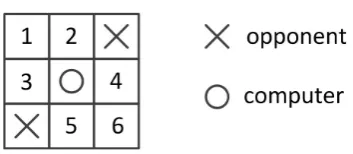
Figure 1. RPS in Tic-Tac-Toe game.
computer’s turn to move. The computer can move to one of 6 possible positions, labeled 1 - 6. If the computer takes 1, then the opponent can take 6, which blocks the diagonal and opens up a vertical and a horizontal to win.
However, RPS does not have this ability to strategically look beyond a few steps. Instead, RPS employs a large number of simulated playouts t=1,2,
and estimates the expected score of move i, for
i
=
1- 6
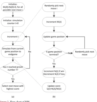
. Figure 2(a) describes the flow chart of RPS and (b) provides the details of function block “simulate from current game position to endgame”.Denote M ti
( )
the number of times that move i has been picked up to playout t and N ti( )
the number of wins minus the number of losses. Initially,( )
0( )
0 0i i
M =N = for all i. Each playout starts with the current game position. RPS randomly picks next move i and increments M ti
( )
by 1. RPS then picks a sequence of random moves for the computer and the opponent until the game ends. If the computer wins, then N ti( )
increments by 1; if the computer loses, then N ti( )
decrements by 1; otherwise, N ti( )
is unchanged. The score is calculated as follows,( )
i( )
( )
.i
i N t S t
M t
= (1)
When the preset number of playouts T has been reached, RPS selects the move i* with the highest score,
( )
* argmax .
i i
i = S T (2)
2.2. Probability Analysis
To assess the performance of RPS, we calculate s0,i, the expected score of move
i from the current game position 0. To simplify the notation, s0,i is
some-times reduced to si. Denote 1 the game position after move i from 0, where subscript 1 indicates that 1 is on level-1 from the starting position 0 on level-0. There are multiple game positions on level-1 and 1 is one of them. Denote K1 the number of legal moves from position 1. Because in a simu-lated playout RPS uniformly randomly selects the next move of the opponent, we have the following recursive equation
1
0 1 1
1
, ,
1
1 K ,
i j
j
s s s
K =
= =
∑
(3)
where s1,j is the expected score of move j from 1. Equation (3) can be
DOI: 10.4236/jilsa.2018.102004 50 Journal of Intelligent Learning Systems and Applications
Figure 2. Flow chart of RPS.
positions are reached. A position is terminal if the game ends at the position, and the game result (loss, draw, win) determines the expected score of the ter-minal position to be −1,0,1, respectively.
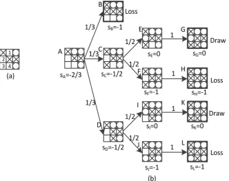
While Equation (3) starts from the current position 0, it is solved by walk-ing backwards from the terminal positions. An example of solvwalk-ing Equation (3) is illustrated in Figure 3, where (a) depicts the current game position 0 and 4 possible moves and (b) shows the calculation of s0,1.
Specifically, the game position 1 after move 1 from 0 is labeled as A, which is expanded into KA=3 next level positions B C D, , . B is a terminal position (loss), so sB= −1. C is further expanded into KC =2 next level posi-tions E, F. E leads to a terminal position G (draw) where sE=sG=0. F leads to a terminal position H (loss), so sF =sH = −1. Thus, from Equation (3),
(
)
1 1 .
2
C E F
C
s s s
K
= + = −
Similarly, D is further expanded into KD =2 next level positions I, J. I leads to a terminal position K (draw) where sI =sK =0. J leads to a terminal position
L (loss), so sJ =sL = −1. Thus,
(
)
1 1 .
2
D I J
D
s s s
K
DOI: 10.4236/jilsa.2018.102004 51 Journal of Intelligent Learning Systems and Applications
Figure 3. Example of calculating expected score of a move with recursive Equation (3). A terminal position is marked by a thick square.
Finally, from Equation (3),
(
)
,1 0
1 2.
3
A B C D
A
s s s s s
K
= = + + = −
(4)
Using the same recursive approach, we can obtain
0,2 0,3 0,4
1, 2, 1.
3 3 3
s = − s = − s = − (5)
Because s0,2=s0,4>s0,1=s0,3, according to Equation (2) RPS selects either
move 2 or 4 with equal probability as the next move from 0.
2.3. Simulation Results
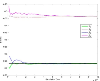
We expect that( )
lim .
i t i
s = →∞S t (6)
Equation (6) states that S ti
( )
given in (1) converges to si, the expected score calculated with the recursive analysis model (3) as the number of playouts increases. We next validate (6) with simulation.DOI: 10.4236/jilsa.2018.102004 52 Journal of Intelligent Learning Systems and Applications
Figure 4. Comparison of simulation results and analysis model. The black straight lines represent s1 to s4, the expected scores calculated with the analysis model (4) (5).
3. From Random Playout Search to Monte Carlo Tree Search
3.1. Expansion of Search Depth in RPS
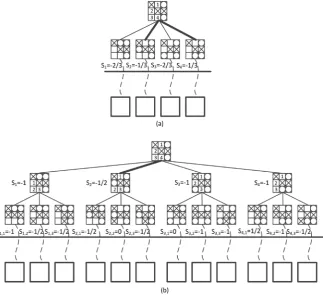
The above analysis and simulation show that for the simple game position in Figure 3(a), RPS selects either move 2 or 4 as the next move, even though only 2 is the right move. We have examined other game positions and found that RPS is often not a winning strategy. Figure 5 lists additional examples of game posi-tions for which RPS fails to find out the right move.
The reason of RPS failure in those game positions is that in the simulated playouts RPS assumes that the opponent randomly picks its moves. However, in the actual game an intelligent opponent does not move randomly. As a result, the prediction ability of RPS is distorted. In the example of Figure 3(b), when calculating sA, it is assumed that the opponent moves to B, C, D with equal probability. However, it is obvious that an intelligent opponent will move to B to win the game and never bother with C, D. The same thing happens in the RPS simulated playouts.
One way to overcome the prediction distortion is to expand the search depth of RPS. Take Figure 3(a) for example. So far RPS only keeps the scores of 4 possible level-1 moves from the current game position. Playouts are simulated from these 4 moves, but RPS does not keep track of the scores below level-1. In this case, the search depth is 1, as illustrated in Figure 6(a), where the winner moves are marked with the thick lines and the dashed lines represent simulated playouts from one position to a terminal position shown as a thick square.
DOI: 10.4236/jilsa.2018.102004 53 Journal of Intelligent Learning Systems and Applications
Figure 5. Additional examples where RPS fails to find out the right move. In each example, move 1 is the right move, but RPS selects move 2 because move 2 has a higher score than move 1.
Figure 6. Expansion of search depth of RPS: search depth = 1 in (a) and 2 in (b). In (a), S1
is what is labeled as SA in Figure 3.
the level-2 moves, which are obtained from the simulated playouts. The scores of the level-1 moves are calculated from those of the level-2 moves with the mini-max principle. That is, the opponent selects the best move, i.e., with minimum score, instead of a random move on level-2,
( )
min1,2,3 ,( )
,i j i j
S t = = S t (7)
for i=1, ,4 . In comparison, when the search depth is 1, although RPS does
not keep track of Si j,
( )
t , in effect S ti( )
is estimated to be( )
,( )
1,2,3
1 .
3
i i j
j
S t S t
=
=
∑
(8) [image:8.595.212.536.200.495.2]DOI: 10.4236/jilsa.2018.102004 54 Journal of Intelligent Learning Systems and Applications Figure 6(b) shows that now RPS selects the right move (2), as opposed to either move 2 or 4 in Figure 6(a). Through simulation and analysis, we confirm that RPS is able to select the right move for the other game positions of Figure 5.
3.2. Brief Summary of MCTS
The idea of expanding the search depth can be generalized to mean that a good algorithm should search beyond the level-1 moves. MCTS takes this idea even further. Starting from the current game position, called the root node, the MCTS algorithm gradually builds a search tree through a number of iterations and stops when some computational budget is met. Similar to the one shown in Fig-ure 6, a search tree consists of nodes representing game positions and directed links each connecting a parent and a child nodes where the game position changes from the parent node to the child node after a move is taken. Every node j in the search tree keeps the total score it gets Xj and the number of times it has been visited nj.
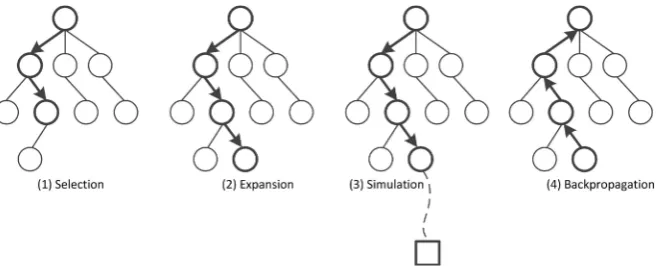
Each iteration in MCTS consists of four steps as illustrated in Figure 7. 1) Selection: A child node is selected recursively, according to a tree policy, from the root node to a leaf node, i.e., a node on the boundary of the search tree. 2) Expansion: A new node is added to the search tree as a child node of the leaf node.
3) Simulation: A simulated playout runs from the new node until the game ends, according to a default policy. The default policy is simply RPS, i.e., ran-domly selecting moves between the computer and the opponent. The simula-tion result determines a simulasimula-tion score: +1 for win, −1 for loss, and 0 for draw.
4) Backpropagation: The simulation score (+1, −1, or 0) is backpropagated from the new node to the root node through the search tree to update their scores. A simple algorithm is that the score is added to Xj of every node j along the search tree.
[image:9.595.211.541.563.696.2]Recall that the nodes from the new node to the terminal node are outside the boundary of the search tree. Any node outside the boundary of the search tree does not keep track of any score.
DOI: 10.4236/jilsa.2018.102004 55 Journal of Intelligent Learning Systems and Applications
The most popular tree policy in MCTS is based on the Upper Confidence Bounds applied to Trees (UCT) algorithm [9][10] whose idea is to focus the search on more promising moves and meanwhile explore unvisited game posi-tions. To describe the UCT algorithm, consider (1) of Figure 7. The root node has three child nodes, j = 1, 2, 3, and selects the one that maximizes the UCB score
2ln
1 j ,
j j
X n
UCB C
n n
= + (9)
where Xj is the total score of child node j, nj the number of times that child node j has been tried, and
n
=
∑
jn
j the total number of times that all child nodes have been tried. The first term average scorej j j X S n
= (10)
aims to exploit higher-reward moves (exploitation), while the second term 2ln
j
n
n encourages examining less-visited moves (exploration), and parameter
C balances exploitation and exploration.
After the algorithm stops, the child node of the root node with the highest av-erage score Sj is selected and the corresponding move from the root node to the selected child node is taken in the actual game.
4. Monte Carlo Tree Search in Gomoku Game
An important theoretical result [8] is that given enough run time and memory, MCTS converges to the optimal tree and therefore results in the optimal move. As shown in Figure 7, the search tree adds one node in the expansion step of every iteration. Within the search tree, UCT selects nodes on the basis of their scores and can thus identify moves of great promise. Outside the boundary of the search tree, MCTS uses RPS in the simulation step. The reason that MCTS converges to the optimal move is that with an infinite amount of search all poss-ible game positions are added to the search tree and that UCT in effect behaves like minimax, which is optimal.
In practice, however, MCTS is limited by computational resource and the search tree is a small subset of the entire game position space. Therefore, MCTS has to rely on RPS to explore a large game position space that is outside the search tree. From the study of Tic-Tac-Toe we learn that a major drawback of RPS is that it assumes the opponent is playing randomly when in fact it is possi-ble that the opponent knows exactly what it should do strategically.
To study MCTS, we need more sophisticated games than Tic-Tac-Toe. In this section, we play Gomoku and see how the insight from the study of Tic-Tac-Toe applies here.
4.1. Sudden Death/Win and Prediction Distortion
DOI: 10.4236/jilsa.2018.102004 56 Journal of Intelligent Learning Systems and Applications
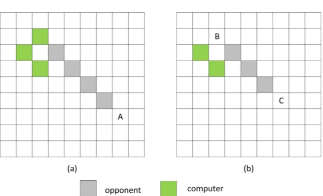
Figure 8. Illustration of sudden death in Gomoku: (a) level-2 and (b) level-4.
computer’s turn to move. In (a), without taking move A, the computer loses in two steps. In (b), without taking move B or C, the computer loses in four steps. On the other hand, if the computer is black and the opponent is green in Figure 8, then the computer wins in one step in (a) by taking move A and wins in three steps in (b) by taking move B or C.
Definition 1. Level-k sudden death or sudden win
A level-k sudden death is a game position where the computer will lose the game in k steps if the computer does not take one of some subset of moves. A level-k sudden win is a game position where the computer will win the game in k
steps if the computer takes one of some subset of moves.
The subset of moves is called decisive moves. The level k is the number of steps that results in a terminal position from the current game position. k is even for sudden death and odd for sudden win. k is a small number for sudden death or win; otherwise, death or win is not “sudden”. More importantly, because of computational resource constraints, it is impractical to detect definite death or win for a large k. In Figure 8, the game position is a level-2 sudden death in (a) and a level-4 sudden death in (b).
One way to detect a level-k sudden death or win is to employ a level-k mini-max search, a slightly modified version of minimini-max search. Specifically, starting from the current game position (root node at level-0), repeatedly expand to the next level by adding the child nodes that represent all the possible next moves from the parent node. Node expansion ends at level-k. A node of terminal posi-tion is assigned a score of −1, 0, 1 as in Secposi-tion 2.2. If a node at level-k is not a terminal position, it is assigned a score of 0, because its state is undetermined. Backpropagate the scores to the root node according to the minimax principle.
DOI: 10.4236/jilsa.2018.102004 57 Journal of Intelligent Learning Systems and Applications
Figure 9. Illustration of level-k minimax search.
principle is that a operation of selecting the minimum or maximum score is ap-plied at every node in alternate levels backwards from level-k. The score of a node at level-4 is the maximum of the scores of its child nodes at level-5 because it is the computer’s turn to move. The score of a node at level-3 is the minimum of the scores of its child nodes at level-4 because it is the opponent’s turn to move, and so on. In Figure 9 A1 is a decision move that leads to a level-5 sud-den win.
Proposition 2. Any level-k sudden death or win is detectable with the level-k
minimax search.
Proof. We focus on sudden win in the proof. The case of sudden death can be proved similarly.
For a level-k sudden win to exist, one of the child nodes of the root node (e.g., 1
A in Figure 9), say node N1,1 at level-1, must be a decisive move that leads to a definite win in level-k. Because it is the opponent’s turn to move at level-1, all
of the child nodes of N1,1 at level-2 (e.g., B B1, 2 in Figure 9), say node 2,1, 2,2,
N N , must each lead to a definite win. For this to happen, at least one of
the child nodes of N2,1 at level-3 (e.g., C1 in Figure 9), say node N3,1, must lead to a definite win so that the opponent has no valid move to avoid the com-puter’s win, and at least one of the child nodes of N2,2 at level-3 (e.g., C3 in Figure 9), say node N3,2, must lead to a definite win, and so on. The above logic applies to each of N N3,1, 3,2,. For example, all of the child nodes of N3,1 (e.g., D D1, 2 in Figure 9) must each lead to a definite win, and at least one child node of each of these nodes (e.g., E E1, 4 in Figure 9) must lead to a definite win. The process repeats until level-k is reached.
sud-DOI: 10.4236/jilsa.2018.102004 58 Journal of Intelligent Learning Systems and Applications
den win. □
Recall from Section 3.2 that MCTS selects the move on the basis of the average scores of the child nodes of the root node (10). In general, the average scores of the child nodes of the root node are rarely equal to the scores of those nodes in a level-k minimax search precisely. However, prediction distortion is not severe if the discrepancy between the two scores does not make MCTS to select a differ-ent child node from what the level-k minimax search would select. It should be pointed out that the level-k minimax search is not necessarily superior to MCTS in all game positions. However, in the presence of sudden death or win, if MCTS selects a move different from the choice of the level-k minimax search, then by definition MCTS fails to make a decisive move. Hence we have the following proposition.
Proposition 3. MCTS fails to detect a level-k sudden death or win if the aver-age scores (10) of the child nodes of the root node are sufficiently deviated from their scores in the level-k minimax search that a decisive move is not selected in MCTS.
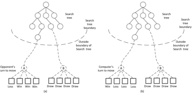
Because of computational resource constraints, the search tree in MCTS is a subset of the entire state space. Random moves are applied in the simulation outside the boundary of the search tree, therefore potentially causing prediction distortion as learned in the RPS analysis. Figure 10 illustrates two examples. In (a), it is the opponent’s turn to move in nodes A and B. Simulations through node A backpropagate higher scores than through node B, making the path through A deceptively more promising, although in reality A is a loss position and B is a draw. If the opponent randomly selects its move, then on average A is better than B. However, if the opponent is intelligent, it selects the move that results in the computer’s immediate loss. In this example, A is a trap that results in computer’s sudden death. In (b), it is the computer’s turn to move in nodes A
and B. Simulations through node A backpropagate lower scores than through node B, making the path through A deceptively less favorable, although in reality
[image:13.595.209.540.547.708.2]A is a win position and B is a draw. If the computer randomly selects its move, then on average A is worse than B. However, as the game progresses toward A,
DOI: 10.4236/jilsa.2018.102004 59 Journal of Intelligent Learning Systems and Applications
the computer will eventually select the move that results in the computer’s im-mediate win. This is an example of sudden win for the computer. Furthermore, even for the nodes within the search tree boundary, their scores may not con-verge to the minimax scores if not enough simulation iterations have been taken.
Clearly as the level increases, it becomes more difficult to discover sudden death/win. In our implementation of MCTS playing Gomoku, we find that MCTS frequently discovers level-1 and level-3 sudden win and level-2 sudden death, but often unable to discovery level-4 sudden death. We will analyze the simulation performance of MCTS next.
4.2. Simulation Results
We have simulated the MCTS algorithm in Java to play Gomoku on an K K×
board. The implementation details are described in Appendix A. We report the simulation results in this section.
4.2.1. Methodology
We do not model the computational resource constraint in terms of precise memory or runtime. Instead we vary the number of iterations T. We find that the run time increases roughly linearly with T and that the Java program runs into heap memory errors when T exceeds some threshold. For example, for
9
K= , the run time is between 7 to 10 seconds for every move at T=30000, and a further increase to T=40000 causes the out of memory error. In con-trast, for K=11, the Java program can only run T =10000 before hitting the memory error. Therefore, we use parameter T to represent the consumed com-putational resource, and K to represent the complexity of the game.
We are interested in the performance of MCTS in dealing with sudden death/win. To report the win rate of an entire game, it would depend on the strength of the opponent, a quantity difficult to measure consistently. Therefore, we let a human opponent to play the game long enough to encounter various sudden death/win scenarios and record the fraction of times that the program detects sudden death/win. Detecting sudden death means that MCTS anticipates the threat of an upcoming sudden death and takes a move to avoid it. Detecting sudden win means that MCTS anticipates the opportunity of an upcoming sud-den win and takes a move to exploit it and win the game.
4.2.2. Result Summary
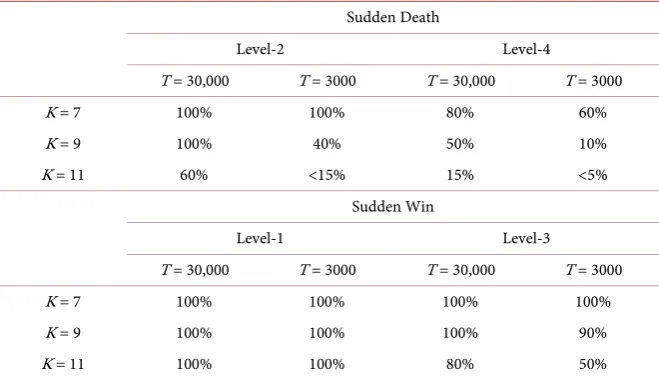
The simulation results are summarized in Table 11. We make the following ob-servations.
• Detecting level-4 sudden death is more difficult than detecting level-2 sudden death. The detection rate drops drastically as the game complexity, represented by K, increases. On the other hand, the detection rate drops drastically as the computational resource, represented by T, decrease.
DOI: 10.4236/jilsa.2018.102004 60 Journal of Intelligent Learning Systems and Applications
Table 1. Detection rate of sudden death/win of MCTS.
Sudden Death
Level-2 Level-4
T = 30,000 T = 3000 T = 30,000 T = 3000
K = 7 100% 100% 80% 60%
K = 9 100% 40% 50% 10%
K = 11 60% <15% 15% <5%
Sudden Win
Level-1 Level-3
T = 30,000 T = 3000 T = 30,000 T = 3000
K = 7 100% 100% 100% 100%
K = 9 100% 100% 100% 90%
K = 11 100% 100% 80% 50%
• There seems to be a tipping point beyond which the detection rate of sudden death is so low that MCTS is useless. For example, for T = 30,000, the tipping point is around K = 7 to 9.
• The detection rate is not symmetric between sudden death and sudden win. Indeed, it seems much easier to detect sudden win than to detect sudden death. In particular, MCTS is always able to detect level-1 sudden win. Moreover, at a first glance, one may expect the detection rate of level-2 den death to be higher than that of level-3 sudden win, because level-3 sud-den win involves more steps to search through. However, it turns out that detecting level-3 sudden win is more robust than detecting level-2 sudden death in a variety of K, T scenarios. We will further investigate this pheno-menon by looking deeper into the scores in MCTS iterations.
• Not shown in Table 1, we observe that when T is small, e.g., T = 3000, and K is large, e.g., K = 9, sometimes MCTS takes seemingly random positions when there are no sudden death/win moves. Furthermore, when K = 11, MCTS often miss the opportunity of seizing level-3 win positions; how-ever, conditional on it already getting into a level-3 win position, MCTS has high probability to exploit the level-3 win opportunity. Therefore, given the computational resource constraint, it is challenging for our Java implementation of MCTS to handle the complexity of a 11 × 11 or larger board.
4.2.3. Level-4 Sudden Death
To investigate the reason that MCTS fails to detect level-4 sudden death, we next examine a specific scenario shown in Figure 11 with K = 9. Shown on the left side of the figure is the current game position, a level-4 sudden death situation. It is now the computer’s turn to move. The correct move should be either B or
DOI: 10.4236/jilsa.2018.102004 61 Journal of Intelligent Learning Systems and Applications
Figure 11. An example of level-4 sudden death in Gomoku.
The moves A B C, , correspond to three child nodes of the root node, represented by three circles labeled as A B C, , in Figure 11. To understand why MCTS chooses node A over node B or C, we plot the MCTS statistics of the three nodes in Figure 12. We observe that node A achieves a higher average score than node B or C does and is visited much more frequently.
This observation may be puzzling, because position A leads to level-3 sudden win, after the computer takes A. So, wouldn’t the opponent take B or C therefore resulting in computer’s loss? These two possible moves are represented by two child nodes of node A, labeled as A1, A2 in Figure 11. The statistics of nodes A1,
A2 are also plotted in Figure 12. We note that the average scores of nodes A1,
A2 are indeed quite negative, indicating that A1, A2 likely result in computer’s loss as expected.
To understand why the low, negative scores of A1, A2 fail to bring down the score of node A, we plot in Figure 13 the MCTS statistics of all the child nodes of node A when the simulation stops at T = 30,000. Among all the child nodes, node A1 is of index 15 and node A2 of index 43. We note that MCTS indeed vis-its A1, A2 much more frequently than other child nodes of node A and that the total scores of A1 and A2 are quite low, both being expected from the exploita-tion principle of the UCT algorithm (9).
DOI: 10.4236/jilsa.2018.102004 62 Journal of Intelligent Learning Systems and Applications
Figure 12. Average scores and numbers of visits of nodes A, B, C, A1, A2 of Figure 11 as the MCTS simulation progresses.
MCTS simulation), the scores of A1 and A2 would eventually dominate the score of their parent node A so that it would be lower than the score of node B
DOI: 10.4236/jilsa.2018.102004 63 Journal of Intelligent Learning Systems and Applications
Figure 13. Total scores and numbers of visits of all the child nodes of node A of Figure 11 at the end of simulation.
DOI: 10.4236/jilsa.2018.102004 64 Journal of Intelligent Learning Systems and Applications
4.2.4. Level-2 Sudden Death versus Level-3 Sudden Win
The example scenario in Figure 14 with K = 11 shows how MCTS fails to detect level-2 sudden death while pursuing level-3 sudden win. Shown on the left side of the figure is the current game position, a level-2 sudden death situation. It is now the computer’s turn to move. The correct move should be B to avoid level-2 sudden death. However, after examining all available positions on the board with T = 10,000, MCTS decides to take position A to pursue level-3 sudden win.
The moves A, B correspond to two child nodes of the root node, represented by two circles labeled as A, B in Figure 14. Figure 15 plots the MCTS statistics of the two nodes. We observe that node A achieves a higher average score than node B does and is visited much more frequently.
Figure 16 plots the MCTS statistics of all the child nodes of node A when the simulation stops at T = 10,000. Among all the child nodes, node A1 is of index 56. We note that MCTS indeed visits A1 more frequently than any other child node and the total score of A1 is the lowest, similar to what we have observed in Figure 13. However, the difference between the child nodes is not as significant. The reason is probably that K is larger and T is smaller in this example and as a result MCTS is still biased towards exploration and exploitation has not been in effect.
The difference of the statistics of nodes A and B in Figure 15, however, is quite minor. In fact, we note that towards the end of the simulation, the average score of B increases while that of A decreases and MCTS visits node B increa-singly more often, indicating that if more computational resource were available to allow T to go further beyond 10,000, then node B would probably overtake node A as the winner and MCTS would find the correct move and overcome level-2 sudden death.
5. An Improved MCTS Algorithm to Address Sudden
Death/Win
[image:19.595.206.538.552.702.2]The issue of sudden death/win is a known problem for MCTS [11][12]. In [13], the authors propose that if there is a move that leads to an immediate win or
DOI: 10.4236/jilsa.2018.102004 65 Journal of Intelligent Learning Systems and Applications
Figure 15. Average scores and numbers of visits of nodes A, B, A1 of Figure 14 as the MCTS simulation progresses.
DOI: 10.4236/jilsa.2018.102004 66 Journal of Intelligent Learning Systems and Applications
Figure 16. Total scores and numbers of visits of all the child nodes of node A of Figure 14 at the end of simulation.
DOI: 10.4236/jilsa.2018.102004 67 Journal of Intelligent Learning Systems and Applications
5.1. Basic Idea
To identify a level-k sudden death/win, we have to use a minimax search of depth k starting from the root node [11]. One brute-force algorithm, as shown in Figure 17(a), is that when the computer enters a new root node, it first runs the minimax search; if there is a sudden death/win within k steps, then follows the minimax strategy to take sudden win or avoid sudden death; otherwise, proceed with MCTS.
However, the computational costs of the minimax search would be significant even for a modest k. Carrying out the minimax search for every new root node reduces the computational resource left for MCTS. The key idea of our proposal is to not burden MCTS with the minimax search until it becomes necessary.
Figure 17(b) shows the flow chart of the improved MCTS algorithm. When the computer enters a new root node, it carries out MCTS. At the end of the si-mulation step of every MCTS iteration, if the number of steps from the root node to the terminal position exceeds k, then continue to the next MCTS
[image:22.595.59.539.311.706.2]DOI: 10.4236/jilsa.2018.102004 68 Journal of Intelligent Learning Systems and Applications
iteration; otherwise, run the minimax search from the root node and follow the algorithm of Figure 17(a). In our implementation, we run a single minimax search of depth k to cover both level-k sudden death and level-
(
k−1)
sudden win for even k.From Proposition 2 the brute-force algorithm is guaranteed to detect any lev-el-k sudden death or win. However, the improved MCTS algorithm can only guarantee the detectability with probability.
Proposition 4. Any level-k sudden death or win is detectable, with probabili-ty, with the improved MCTS algorithm in Figure 17(b), where the probability depends on the number of MCTS iterations, the complexity of the game, and the value of k.
The reason of “guarantee with probability” in Proposition 4 is that the im-proved MCTS algorithm needs to encounter a terminal node within level-k in at least one of the many iterations before a minimax search is triggered. In Gomo-ku, we find that the probability is close to 1 when the number of iterations is large, the board size is modest, and depth k is a small number, e.g., T = 30,000, K
= 9, k = 4.
5.2. Simulation Results
We have implemented the improved MCTS algorithm in JAVA. The implemen-tation includes a minimax search of depth 4, and we confirm that the program is able to always detect any level-2/4 sudden death and level-1/3 sudden win. To assess the computational resource used in the minimax search of depth 4 and the overall MCTS algorithm, we record the total elapsed time of every MCTS step, which includes T simulations and possibly a minimax search, as well as the elapsed time of every minimax search when it happens. Figure 18 shows that the cumulative distribution functions (CDF) of the two elapsed times for the case of
T = 30,000, K = 9.
We observe that the elapsed time of a minimax search is pretty uniformly distributed from 0 to about 1.8 seconds and that the elapsed time of a MCTS step is either small (below 2 seconds) or quite large (above 6 seconds), where the small value corresponds to the scenarios where MCTS can find easy moves to win the game (level-1 or level-3 sudden win). On average, a single minimax search is about 1/6 of the entire MCTS 30,000 simulations. As the depth in-creases, the minimax search will be exponentially expensive. Therefore, the advantage of the proposed algorithm over the brute-force algorithm could be significant.
5.3. Heuristic Strategies to Enhance Performance
DOI: 10.4236/jilsa.2018.102004 69 Journal of Intelligent Learning Systems and Applications
Figure 18. CDF of the total elapsed time in every MCTS step and the elapsed time of a minimax search.
DOI: 10.4236/jilsa.2018.102004 70 Journal of Intelligent Learning Systems and Applications
Suppose that in one iteration of MCTS a terminal node of loss (or win) is en-countered within depth k from the root node, indicating the potential presence of sudden death (or win). Mark the child node of the root node selected in that iteration as a potential sudden death (or win) move.
Consider the first heuristic strategy. Instead of triggering a minimax search immediately as in Figure 17(b), we continue to run MCTS for some number of iterations and then apply the following two rules.
1) For the subset of child nodes of the root node whose average scores are in the top x1 percentile and that have been marked as a potential sudden death move, run a minimax search of depth k−1 from each of them. If the minimax score of a child node in the subset is equal to −1, then mark it as a sudden death move and refrain from selecting it in subsequent MCTS iterations. Continue to run MCTS.
2) For the subset of child nodes of the root node whose average scores are in the top x2 percentile and that have been marked as a potential sudden win move, run a minimax search of depth k−1 from each of them. If the minimax score of any of them is equal to 1, then mark the child node as a sudden win move, which is the best move to select, and stop MCTS. Otherwise, continue to run MCTS.
Rule 1 is to prevent a sudden death move from prevailing in MCTS node se-lection. For example, move A in Figure 11 will be detected and discarded, and therefore will not prevail over move B or C. Rule 2 is to discover a sudden win move and to end MCTS sooner. Here x x1, 2 are heuristic numbers that are used to trade off the reduction in minimax search with the improvement of MCTS ef-fectiveness.
Consider the second heuristic strategy. Instead of running MCTS for some number of iterations, applying the above two rules and then continuing MCTS as in the first strategy, we can run MCTS to the end and then apply the following two similar rules.
1) For the child node of the root node with the highest average score, if it has been marked as a potential sudden death move, run a minimax search of depth
1
k− . If its minimax score is equal to −1, then discard it, proceed to the child node with the second highest average score and repeat this rule. Otherwise, pro-ceed to the next rule.
2) For the subset of child nodes of the root node whose average scores are in the top x2 percentile and that have been marked as potential sudden win moves, run a minimax search of depth k−1 from each of them. If the minimax score of any of them is equal to 1, then select the move. Otherwise, select the move according to the MCTS rule.
The performance of the above two heuristic strategy can be assessed with the following proposition.
DOI: 10.4236/jilsa.2018.102004 71 Journal of Intelligent Learning Systems and Applications 17(b). Its capability to detect a sudden win improves as x2 increases, and is in general strictly weaker than the improved MCTS algorithm, except in the special case where x2=100 in which case it has the same sudden win detection capa-bility.
In Gomoku, if x2 is a small number, the complexity reduction over the im-proved algorithm of Figure 17(b) is in the order of
O K
( )
2 , because the size of the subset of the child nodes from which a minimax search actually runs is roughly 1 K2 of the size of the total set. Even for a modest board size K, e.g.,9
K= , the reduction is significant.
6. Conclusions
In this paper we analyze the MCTS algorithm by playing two games, Tic-Tac-Toe and Gomoku. Our study starts with a simple version of MCTS, called RPS. We find that the random playout search is fundamentally different from the optimal minimax search and, as a result, RPS may fail to discover the correct moves even in a very simple game of Tic-Tac-Toe. Both the probability analysis and simula-tion have confirmed our discovery.
We continue our studies with the full version of MCTS to play Gomoku. We find that while MCTS has shown great success in playing more sophisticated games like Go, it is not effective to address the problem of sudden death/win, which ironically does not often appear in Go, but is quite common on simple games like Tic-Tac-Toe and Gomoku. The main reason that MCTS fails to detect sudden death/win lies in the random playout search nature of MCTS. Therefore, although MCTS in theory converges to the optimal minimax search, with computational resource constraints in reality, MCTS has to rely on RPS as an important step in its simulation search step, therefore suffering from the same fundamental problem as RPS and not necessarily always being a winning strategy.
Our simulation studies use the board size and number of simulations to represent the game complexity and computational resource respectively. By ex-amining the detailed statistics of the scores in MCTS, we investigate a variety of scenarios where MCTS fails to detect level-2 and level-4 sudden death. Finally, we have proposed an improved MCTS algorithm by incorporating minimax search to address the problem of sudden death/win. Our simulation has con-firmed the effectiveness of the proposed algorithm. We provide an estimate of the additional computational costs of this new algorithm to detect sudden death/win and present two heuristic strategies to reduce the minimax search complexity and to enhance the MCTS effectiveness.
DOI: 10.4236/jilsa.2018.102004 72 Journal of Intelligent Learning Systems and Applications
References
[1] Schaeffer, J., Müller, M. and Kishimoto, A. (2014) Go-Bot, Go. IEEE Spectrum, 51, 48-53. https://doi.org/10.1109/MSPEC.2014.6840803
[2] https://en.wikipedia.org/wiki/Computer_Go
[3] Nandy, A. and Biswas, M. (2018) Google’s DeepMind and the Future of Reinforce-ment Learning. In: Reinforcement Learning, Apress, Berkeley, 155-163.
https://doi.org/10.1007/978-1-4842-3285-9_6
[4] Silver, D., et al. (2017) Mastering the Game of Go without Human Knowledge. Na-ture, 550, 354-359. https://doi.org/10.1038/nature24270
[5] Coulom, R. (2006) Efficient Selectivity and Backup Operators in Monte-Carlo Tree Search. In: van den Herik, H.J., Ciancarini, P. and Donkers, H.H.L.M., Eds., Com-puters and Games. CG 2006. Lecture Notes in Computer Science, vol 4630, Sprin-ger, Berlin, Heidelberg, 72-83.
[6] Kocsis, L. and Szepesvári, C. (2006) Bandit Based Monte-Carlo Planning. In: Fürnkranz, J., Scheffer, T. and Spiliopoulou, M., Eds., Machine Learning: ECML
2006. ECML 2006. Lecture Notes in Computer Science, vol 4212, Springer, Berlin, Heidelberg, 282-293. https://doi.org/10.1007/11871842_29
[7] Chaslot, G.M.J-B., Saito, J.-T., Bouzy, B., Uiterwijk, J.W.H.M. and van den Herik, H.J. (2006) Monte-Carlo Strategies for Computer Go. Proceedings of the 18th Be-NeLux Conference on Artificial Intelligence, Belgium, 2006, 83-90.
[8] Browne, C., Powley, E., Whitehouse, D., Lucas, S., Cowling, P.I., Rohlfshagen, P., Tavener, S., Perez, D., Samthrakis, S. and Colton, S. (2012) A Survey of Monte Carlo Tree Search Methods. IEEE Transactions on Computational Intelligence and AI in Games, 4, 1-49. https://doi.org/10.1109/TCIAIG.2012.2186810
[9] Auer, P., Cesa-Bianchi, N. and Fischer, P. (2002) Finite-Time Analysis of the Mul-ti-Armed Bandit Problem. Machine Learning, 47, 235-256.
https://doi.org/10.1023/A:1013689704352
[10] Chang, H., Fu, M., Hu, J. and Marcus, S. (2005) An Adaptive Sampling Algorithm for Solving Markov Decision Processes. Operations Research, 53, 126-139.
https://doi.org/10.1287/opre.1040.0145
[11] Ramanujan, R., Sabharval, A. and Selman, B. (2010) On Adversarial Search Spaces and Sampling-Based Planning. Proceedings of the 20th International Conference on Automated Planning and Scheduling, Toronto, 12-16 May 2010, 242-245.
[12] Browne, C. (2011) The Dangers of Random Playouts. ICGA Journal, 34, 25-26.
https://doi.org/10.3233/ICG-2011-34105
[13] Teytaud, F. and Teytaud, O. (2010) On the Huge Benefit of Decisive Moves in Monte-Carlo Tree Search Algorithms. Proceedings of IEEE Conference on Compu-tational Intelligence and Games, Copenhagen, 8-21 August 2010, 359-364.
DOI: 10.4236/jilsa.2018.102004 73 Journal of Intelligent Learning Systems and Applications
Appendix A
A. Java Implementation
The following appendix sections describe the Java implementation of the analy-sis and simulation codes used in this study.
A1. Tic-Tac-Toe and Gomoku Game GUI
[image:28.595.208.537.467.717.2]I downloaded a Java program from the Internet, which provides a graphic user interface (GUI) to play Tic-Tac-Toe. I modified the program to play Gomoku. Figure A1 shows a screenshot of the game GUI generated by the program.
The game GUI consists of two panels. The left panel shows two options to play the game: person-to-person or person-to-computer. In this study I am only interested in the latter option. The two colors, black (person) and green (com-puter), show whose turn it is to move. The right panel is a K × K grid to represent the game board.
The program uses an array currentTable[] of length K2 to represent the cur-rent game position, where element curcur-rentTable[i*K+j] is the state of row i and column j of the game board. currentTable[i*K+j] can be in one of three states:
enum TILESTATUS {EMPTY, PERSON, COMPUTER}.
Initially, all elements are EMPTY. When it is the person’s turn to move and the human player clicks on one of the empty grid element, the program changes the corresponding element of currentTable[] to PERSON. When it is the com-puter’s turn to move, the program calls a function.
int choseTile()
which returns an integer index pointing to one of the elements of currentTable[] representing the computer’s move. The program changes the corresponding
DOI: 10.4236/jilsa.2018.102004 74 Journal of Intelligent Learning Systems and Applications
element of currentTable[] to COMPUTER. After every move, the program calls a function
boolean checkWinner(TILESTATUS[] currentTable, int select)
to check whether the game position currentTable has a winner where select is the latest move.
Function choseTile() is where any AI algorithm is implemented. In the Tic-Tac-Toe Java program downloaded from the Internet, the default imple-mentation is to randomly return any index that corresponds to an EMPTY ele-ment. In this study, I have implemented the RPS and MCTS algorithms in cho-seTile(). I will describe our implementation of RPS and MCTS later.
A2. Implementation of Probability Analysis of RPS
I wrote a Java program to calculate the expected score of each move from the current game position of RPS. The Java program is used in the probability analy-sis in Section 2.2.
The calculation is based on the recursive Equation (3). The current game po-sition is represented by the root node and all the legal next-step moves from the current game position by the computer form its immediately child nodes. The Java problem uses a recursive function
float scoreIteration(TURN turn, int select)
to calculate the expected score of the child node presented by currentTable. De-note K the number of EMPTY elements in the root node and index[k] the k-th EMPTY element. The main() function calls scoreIteration() for each of the K child nodes of the root node, k, with turn set to COMPUTER, select set to in-dex[k], and currentTable[index[k]] set to COMPUTER. currentTable[index[k]] is reset to EMPTY after each function call.
The programming idea of scoreIteration() is that if the node is terminal, then return −1, 0, 1 depending on the game outcome; otherwise, expand to its child nodes and call scoreIteration() recursively. When a node expands to its next lev-el child nodes, the number of EMPTY lev-elements decrements by one. The pseudo of scoreIteration() is given as follows.
A3. MCTS and RPS Implementation
I downloaded a Java program from the Internet
(https://code.google.com/archive/p/uct-for-games/source), which implements the MCTS algorithm. I modified the MCTS program to work with the GUI pro-gram, to output various statistics to study the simulation results in Sections 2.3 and 4.2, and to allow flexible alrogithm selection, which will be necessary to im-plement the improved MCTS algorithm of Section 5.
The MCTS Java program defines a class called MCTSNode, which includes a number of variables and methods to implement the algorithm described in Sec-tion 3.2. The most important variables are
int totalScore to store the total score of the node,
DOI: 10.4236/jilsa.2018.102004 75 Journal of Intelligent Learning Systems and Applications
ArrayList<MCTSNode> nextMoves to store an array list pointing to the child nodes of the node,
int indexFromParentNode to store the move that its parent node takes to reach the node,
TILESTATUS[] nodeGameState to store the game position of the node, TILESTATUS nodeTurn to store whose turn it is to move.
The average score of the node is simply totalScore/timesVisited. The most important methods are described below.
Function choseTile() calls bestMCTSMove(), which returns the move chosen by MCTS.
bestMCTSMove() in turn calls runTrial() in each MCTS iteration, in which the game ends in one of three outcomes
enum TURN {PERSON, COMPUTER, DRAW}.
runTrial() calls simulateFrom() to simulate a random playout beyond the tree boundary.
DOI: 10.4236/jilsa.2018.102004 76 Journal of Intelligent Learning Systems and Applications
int levelFromTopNode to store the number of levels from the root node to the node. For a child node of the root node, levelFromTopNode is set to 1.
The only change to implement RPS is that line 5 of function runTrial() is re-placed by
if Node is a leaf node AND levelFromTopNode == 0 then
so that only the root node is expanded to add its child nodes, which are never expanded and are kept as the leaf nodes.
A4. Improved MCTS Implementation
DOI: 10.4236/jilsa.2018.102004 77 Journal of Intelligent Learning Systems and Applications
the MCTSNode class:
int simulationDepth to store the number of steps from the root node to where the game ends in function simulateFrom()
ArrayList<MCTSNode> nextMinimaxMoves to store an array list pointing to the child nodes of the node that are the optimal moves found in the minimax search. nextMinimaxMoves is a subset of nextMoves.
Besides, a static variable is defined:
int MINIMAXSEARCH to indicate whether the minimax search should be taken and whether has been taken.
The changes to functions bestMCTSMove(), runTrial() and simulateFrom() are summarized as follows.
In bestMCTSMove(), lines 3 to 4 are replaced by the following.
In runTrial(), lines 7 to 11 are replaced by the following. Here, constant NUMSIMULATIONDEPTH is the depth k in Figure 17(b)).
In simulateFrom(), the following is added immediately after line 8. simulationDepth ← simulationDepth+1
DOI: 10.4236/jilsa.2018.102004 78 Journal of Intelligent Learning Systems and Applications
NUMSIMULATIONDEPTH. I wrote two versions of minimax(). The first ver-sion uses recurver-sion.