RESEARCH ARTICLE
PERFORMANCE EVALUATION OF MAGNETIC INTERPRETATION TECHNIQUES: METHOD BASED
ON CHARACTERISTIC POSITIONS AND INVERSION INTERPRETATION TECHNIQUES
1,*
Subrahmanyam M.,
1Fekadu Tamiru and
2Satyanarayana K. V. V.
1
Department of Geophysics, Andhra University, Visakhapatnam-530003, India
2
Department of Earth Sciences, Wollega University, Ethiopia, Nekemte
ARTICLE INFO ABSTRACT
Interpretation techniques employed in magnetic data enable in quantifying the subsurface geological bodies for various purposes. Of the various types of them the performance evaluation of methods based on the characteristics positions and inversion techniques were studied in the present paper. The theoretical magnetic data was generated over simple geological bodies of sheet, dike and vertical fault models. The data thus generated has been used for performance study. The anomalies were interpreted with the characteristic positions method for the dike, vertical fault and sheet model where as the inversion method is for the dyke model only. From these interpretation techniques the source parameters were estimated. With the assumed source parameters and estimated, the percent error was determined. The estimated percent errors from the performance evaluations of the techniques showed that the use of characteristics positions method determines the origin with less than ±0.5% error, of all the tabular bodies presented in this paper irrespective of the actual shape of the anomaly and without the knowledge of any prior information. The source parameters estimated for the three simple bodies used in the study are in the acceptable percent errors less than ±10 percent.
Copyright, IJCR, 2013, Academic Journals. All rights reserved.
INTRODUCTION
All existing geophysical exploration methods are based on the physical properties of the subsurface bodies. Geological bodies vary distinctly in these physical properties which laid a foundation for adopting comprehensive geophysical prospecting techniques to solve this kind of problems. Among these, the potential method is a widely studied and oldest of the geophysical methods that are routinely used to solve quickly a wide variety of geological problems for resource explorations or/and structural study purposes. The principal goals of a magnetic study are to detect and quantify changes in magnetic properties at depth and to interpret subsurface geologic structure. Interpretation techniques in magnetic methods for the classical and automated have both advantages and limitations. In both cases the interpretation attempts to determine the physical dimensions of the model, its depth and magnetization contrast through properly developed formulae. The purpose of this study focuses on the performance evaluation of interpretation techniques in magnetic methods for tabular bodies.
In general ambiguity is not peculiar to magnetic method but is pertinent to all geophysical methods. It was discussed by Silva et al.
(2003) as; the peculiarity of magnetic interpretation is that magnetization is not a scalar but a vector property which is related to surface rather than to volume distributions of magnetic poles. As a result, the fundamental ambiguity in magnetic interpretation is more complex because not only the magnetization intensity but also magnetization inclination and declination may couple with parameters defining the source. For the same magnetization intensity, a wide, thin tabular source may produce large or small magnetic anomalies above its centre, depending on whether the magnetization inclination is, respectively, high or low. The major difficulty in interpretation of all geophysical methods is the non-uniqueness problem which is true for
*Corresponding author: [email protected]
magnetic method too. By Gauss’ theorem, if the field distribution is known only on a bounding surface, there are infinitely many equivalent source distributions inside the boundary that can produce the known field. For this reason, Thompson (1982) summarized as the representation of the anomalous magnetic field as due to a subsurface distribution of simple magnetic models is also not unique. Any magnetic field measured on the surface of the earth can be reproduced by an infinitesimally thin zone of magnetic dipoles beneath the surface. This means there is no depth resolution inherent in magnetic field data. A second source for non uniqueness is the fact that magnetic observations are finite in number and are inaccurate. If there is one model that reproduces the data, there are other models that will reproduce the data to the same degree of accuracy.
Quantitative interpretations of magnetic data provide an excellent basis in which geological boundaries and lithologies are being estimated. Gunn (1997) described his suggestion on the automated quantitative interpretation techniques as, it is not certain, however, that many, if any, of the interpretation of depths to the magnetic sources have been made with the accuracy. Numerous interpretation techniques are available in literature for interpreting magnetic anomalies. It is very difficult for the interpreter to choose one among the many to solve magnetic problem since there is no performance evaluation available for most the techniques. Prakasarao and Subrahmanyam (1985) carried out error analysis for the effect of
interpretation over 2D bodies was applied to
2
1
2
D bodies (usingGrant and West equation, 1965). Though each interpretation of magnetic anomaly has its own limitation, applying appropriate technique to obtain source body parameter is not an easy task. Every one that applies any of the geophysical interpretation techniques has to understand to what degree it performs to determine the source body parameters. In line to this objective the performance evaluation of magnetic interpretation techniques is necessary. Two magnetic interpretations methods namely the characteristics position method
ISSN: 0975-833X
International Journal of Current Research
Vol. 5, Issue, 03, pp. 617-629, March,2013
INTERNATIONAL JOURNAL
OF CURRENT RESEARCH
Article History:
Received 30th
December, 2012 Received in revised form 29th January, 2013 Accepted 28th
February, 2013 Published online 19th
March, 2013
Key words:
and inversion method are studied for their performance. Subrahmanyam and Prakasarao (2009) suggested that the characteristic positions method considered in this study locate the origin of the source body by the method of circles. The main objective of this paper is to present the performance evaluation of characteristics position and inversion interpretation techniques over tabular bodies.
METHODOLOGY
In this study two magnetic interpretation techniques are used for performance evaluation, one method is based on characteristic position and the other is inversion of magnetic anomaly over dike. The synthetic data were generated for three tabular models with source parameters depth (H) and width (W) for dyke, top (H1) and bottom (H2) depths for vertical fault and depth for sheet (H) and magnetization angle for all model by varying width to depth ratio for dike, bottom depth to top depth ratio for vertical fault and varying to different depths for sheet by varying magnetization angle for the each of the body. The data generated for vertical fault and sheet models were interpreted with the characteristics position technique while the dyke model interpreted with both the methods. The percent error was estimated with the theoretical and determined source parameters in analysing the performance of the techniques considered. The percent error estimated for width and depth for dike, top depth and bottom depth for vertical fault, depth to the top of sheet and origin and magnetization angle for all the three models were plotted to show to what degree of the technique employed performed with in the acceptable range of error.
Theory
Magnetic Interpretation of Simple bodies
Subrahmanyam and Prakasarao (2009) proposed a magnetic interpretation method on the profile anomaly using the relationships between the distance of characteristic position and parameters of the causative tabular sources. The other method is taken from the inversion techniques. The inversion method of (Radhakrishna Murty, and Misra, 1989) on dike bodies considered for performance evaluation.
Methods based on Characteristic positions
[image:2.612.158.458.349.690.2]The method of Subrahmanyam and Prakasarao (2009) has been used here for the performance evaluation of the characteristics method. The method interprets the location of the source by the method of circles and the geometric source parameters are determined by using the relation between certain characteristic positions on the geometric dimensions of the source and also magnetization direction. The entire interpretation method is automated with a computer code and the computer program simply gives the output for location, magnetization direction and geometric dimensions of the tabular sources (Fig.1). Computer program written for this interpretation technique based on the relation between characteristic distances and geometric parameters of the tabular sources is used for performance evaluation. Theoretical magnetic anomalies over sheet, Dike and vertical step are computed for different combination of geometric dimension of the bodies for varying magnetization angles.
Each profile is interpreted with the program and percent errors are computed for the interpreted parameters. The percent errors in each of the parameters for all the geometric models are analyzed for the performance of the techniques.
Theoretical back ground for the method of characteristics
position method
Subrahmanyam and Prakasarao (2009) have developed a method based on the properties of characteristic positions on the magnetic on the magnetic anomaly profiles over simple geometric bodies (Fig 1). The method of circles is used to identify the origin of the source body based on the common properties identified on the anomaly. These properties are related to the characteristic positions on the anomaly curve. The method of interpretation overcomes the limitations associated with the need for a prior knowledge of the origin and datum level. The method splits the anomaly curve into symmetric and antisymmetric components and these components were analyzed for determining the source parameters. Subrahmanyam and Prakasarao (2009) derived mathematical relations between the distances of characteristic positions on the symmetric and antisymmetric components and the source parameters. At zero and ninety degree magnetization angle (00 and 900) the nature of the anomaly curves are symmetric and antisymmetric respectively. For these two cases the procedure outlined for symmetric and antisymmetric components may be adopted.
The general magnetic expression for the models used is the form of;
B
A
F
(1)Where,
F
represents the magnetic anomaly
and
are thegeometric factors A and B are the coefficients of amplitude,
and
have odd and even symmetry with respect to the central axis. Theeffective inclination angle (
F) in the plane of the principal profile is equal to the angle between the magnetization inclination and the plane of the body. Thus, the magnetic expression due to dyke body has the form∆ = ( + ) (2)
Where, = + H − − =1 2ln ( + ) + ( − ) +
=
(1
−
)
(1
−
)
for∆
remanence= (1− ) for ∆ induction
= (1− ) for ∆ and = + − −90 for ∆ remanence = 2 − −90 for ∆ induction = −
for ∆
Where;
∆
-magnetic anomaly -amplitude factor -Index parameterT-total intensity of earth’s magnetic field -susceptibility contrast
′
=
(1
−
)
-it is the component of the earth’s normal flux-inclination of the earth’s magnetic field
-de inclination of the earth’s magnetic field from x-axis
i- inclination of the resultant magnetization,
a-declination of the resultant magnetization from x-axis.
I-resolved direction of the induced component of magnetization in the xz-plane
-remance and induction component of magnetization in xz plan X-distance of the point of observation from the origin,
H-depth to the top of dike, sheet H1-depth to the top of the fault H2-depth to the bottom of the fault 2w-width of dike, t-thickness of sheet
-geological dip
This expression is the modified form and
and
are the symmetric and antisymmetric components of equation (1). The expression of equation (1) is applied for the anomalies of total, vertical and horizontal components of the field and also to any orientation of the body, of the magnetic vector and the direction of the sensor elements of the magnetometer.Magnetic expression for the sheet is given by
∆ ( ) = (3)
Where,
= (1− ) (1− ) for ∆
(remance dominant)
= (1− ) for ∆ induction = (1−
) for ∆ and = + − −90 for ∆ (when remanence is dominant)
= 2 − −90 for ∆ induction = − for ∆
Magnetic expression for the vertical step is given by
∆ ( ) =
1− 2
− 1
2
+ ( 1)
+ ( 2) (4)
= (1− ) (1− ) for ∆
remanence
= (1− ) for ∆ induction
= (1− ) for ∆ and = + − −90 for
∆ remanence
= 2 − −90 for ∆ induction = − for ∆
Characteristic properties of the anomaly curve to fix the correct, quadrant of ( is obtained from the method)
Anomaly Shape Value of
Major positive anomaly towards positive x-axis
=
or (
-3600)Major positive anomaly towards negative x-axis
=-
or –(
+3600)Major negative anomaly towards positive x-axis
=
-1800)Major positive anomaly towards negative x-axis
=-(
+3600)Inversion Method
Sengpiel and Siemon, 2000) have the advantage of yielding a much superior resolution for the given output parameter and the disadvantage that the output parameter may vary with the starting model, so this lack of robustness is always a concern when evaluating an interpretive output. The inverse method is in which source parameters are determined in a direct way from magnetic measurements. Magnetic surveys have been used in investigations of wide range of scales such as tectonic studies, petroleum exploration, in mineral explorations and environmental problems. The inversion of magnetic data constitutes an important step in the quantitative interpretation. The inverse problem in geophysics involves the selection of a geometrical model for which a mathematical formula can be derived to calculate the model response using the initial values of body parameters. Magnetic anomalies are inverted by choosing initial values for the model parameters and calculating increments to improve them iteratively trough techniques of optimization. In inverse modelling, a geometrical model is chosen with initial estimates of the body parameters, and then the process is iteratively advanced until a satisfactory fit is obtained between observed and calculated anomalies. Initial values of the model parameters are assigned by the interpreter, or are implicitly or explicitly determined by the computer. The optimization procedure changes the initial body parameters iteratively to reach a model, which fits the observed data Marobhe, (1989). Inversion routines can be subdivided into two broad groups: linear and non linear. The method and computer program of Radhakrishna Murthy and Misra (1989) is used here for performance evaluation.
Magnetic Inversion of Dike
From the magnetic anomaly profile inversion due to dike, the parameters that to be determined are width, depth to the top of the dike, the origin (the position of the centre of the dike) and . The magnetic anomaly required as an input for the inversion process has the expression from Radhakrishna Murthy and Misra, (1989) and it is given as
∆ ( ) = 2 1− arctan +
−arctan − + ( − ) +
( + ) +
(5)
Where,-magnetic anomaly in any component
J- Intensity of effective magnetization of the two dimensional body x-distance co-ordinates of the anomalies
-geological dip of the body -dip of the effective magnetization
-strike of the body measured from the magnetic north –angle which is a function of
w-half width of the dike, h-depth to the top dike
Dm-direction of measurement (0 for horizontal, for vertical and
for total field) The size factor 2 1− is independent of the length parameters of the dike and direction of magnetization determines 2 . The shape of the magnetic anomaly profile over the dike is defined by the expression in the square brackets. For a given magnetic profile over arbitrary magnetized dike can be produced by a series of dykes of the same depth and width, but with their dips and direction of magnetizations differing which causes some ambiguities.
Performance Evaluation
Characteristics position method
Sheet Model
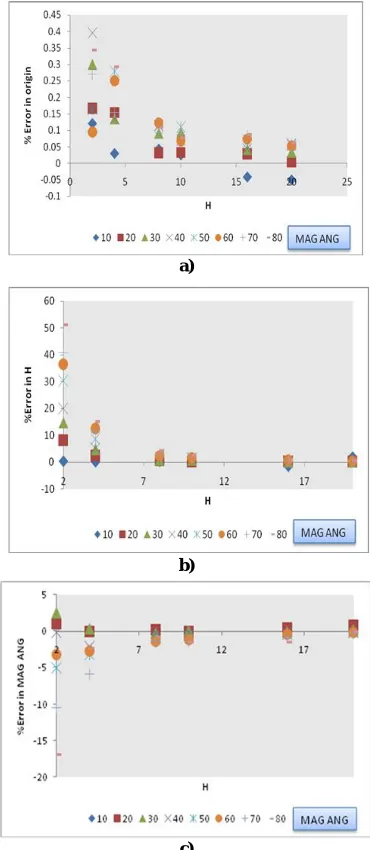
The percent error is the calculation of the difference between the theoretical and interpreted values. The interpreted values are origin, depth and magnetization angle. Fig 2(a) shows the percent error origin against depth. The percent error is less than ±0.4%. For higher values of depth (i.e for deeper bodies) the percent error is almost zero. Fig 2(b) shows the percent error obtained in the depth parameters. The percent error is less than ±10%. However for lower magnetization angles the percent error in depth is a little higher but less than ±20%
with the exception of
80
0. This may be due to the anti-symmetric nature of the curve shape and possibility of error in determination of characteristic positions. The program for the interpretation of anomalies uses interpolation techniques for determining the characteristic positions. Fig 2(c) shows the percent error of magnetization angle against depth for different values of magnetization angles. The error is less than ±5% for shallow as well as deeper bodies for all magnetization directions. Overall the program provides to be effective for interpreting of magnetic anomalies over sheet like modela)
b)
c)
[image:4.612.342.527.285.710.2]Dike model
The magnetic profile data generated for dyke with different width to depth ratio (W/H) for varying magnetization angle were interpreted with the use of characteristic positions method and source parameters were estimated. The source parameters estimated by the method are origin, width, depth and magnetization angle of the dyke for all magnetic profile used as depth to the top the dyke is increasing. The characteristic positions method determines the origin of all the tabular bodies irrespective of the actual shape of the anomaly and without the knowledge of any prior information. The source parameters of the assumed model are determined from the characteristics position of the anomaly. The percent error was determined from the interpreted (estimated) source parameters from the use of characteristics position method and with the actual source parameters assumed during the generation of the data. The discrepancy between the estimated and assumed parameters for the origin, width, depth and magnetization angle is calculated as percent error and it was plotted as in the following figures shown and for all the corresponding model types.
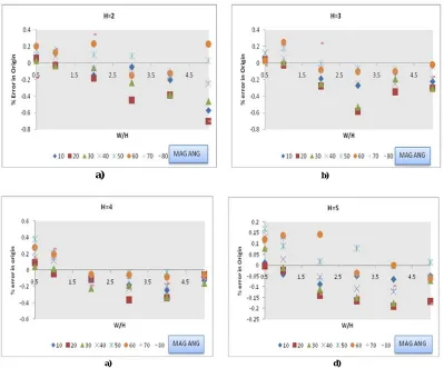
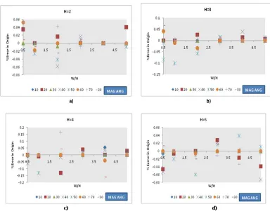
Percent error in the origin
Fig 3(a-d) shows the percent error of origin against the width to depth ratio (W/H) for varied depths to top of the body. From figure, it is observed that the percent error for the origin is less than ±0.6 percent. It is also observed in the figures that as the width to depth ratio increases the percent error in origin decreases and attains percent error less than ±0.2 percent for all the magnetization angle. Thus, the deeper the body is the lesser the error in origin.
Percent error in the width
Fig 4(a-d) shows the percent error in width against width to depth ratio for varied depths to top of the body and for varying magnetization angles. The percent error estimated for width of dyke model by the use of the characteristics position method is almost zero as the depth to the source body is getting deeper and the width to depth ratio increases for the all magnetization angle. Though for very shallow and small values of width to depth ratio the percent error is a little higher for some magnetization angles, but still in acceptable limits.
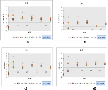
Percent error in the depth
As shown in the figure 5(a) the prcent error in depth slightly increases less than ±10 prcent for the relatively lowest width to depth ratio(W/H). But for the rest of the width to depth ratio and deeper sources, the prcent error found to be less than ±5 prcent for all magnetization direction.
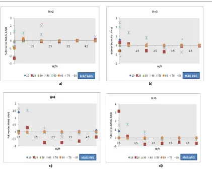
Percent error in the magnetization angle
Fig 6(a-d) presents percent error in magnetization angle against width to depth ratio. It shows that for both shallow and deeper sources the percent error is less than ±2 percent for the entire width to depth ratio values with the exception of H=2 the percent error is less than 6 percent.
a)
b)a) d)
[image:5.612.110.509.342.673.2]a) b)
c) d)
Fig. 4. (a-d) Percent error in width for the dyke model for depths of 2-5 units, H(depth), W(width), W/H(width to depth ratio)
a) b)
c) d)
[image:6.612.125.494.58.368.2] [image:6.612.133.484.397.689.2]Vertical Fault Model
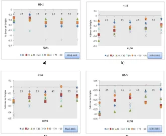
Percent error in origin
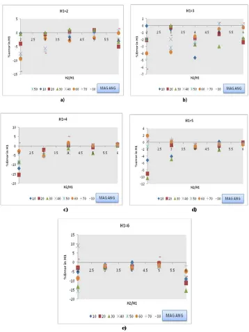
Fig 7(a-e) shows percent errors of origin against the ratio of bottom to top depths of the vertical fault model for varying magnetization angles for varied depth levels of source. The percent error in origin was determined to be less than ±0.5 percent and even decreases as the source become deeper and as H2/H1 ratio increases for all magnetization angles.
Percent error in depth to top
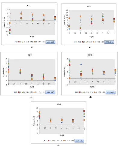
In the Fig 8(a-e) it is shown that percent error in the depth to top of the vertical fault was nearly less than ±15 percent for shallow sources. For deeper source of vertical fault body the percent error is less than ±10 percent and decreases rapidly to less than 5 percent as H2/H1 increases.
a) b)
c) d)
Fig. 6. (a-d) Percent error in the magnetization angle of the dyke model for depth (H1) of 2-5 units, H(depth), W(width), W/H(width to depth ratio)
a) b)
[image:7.612.135.477.49.341.2] [image:7.612.145.475.461.732.2]e)
Fig. 7. (a-e) Percent errors in origin of vertical fault model for top depth (H1) 2 to 6 units and bottom depth (H2), H2/H1 (bottom to top depth ratio)
Percent error in bottom depth
In similar way to the percent error mentioned for depth to the top, the percent error in depth to bottom is shown in Figure 9(a-e). Figure 9 shows H2 relatively higher percent error for shallow sources and it become less than ±10 percent for deeper sources, and decreases rapidly to less than 5 percent as H2/H1 increases.
Percent error in magnetization angle
Fig 10. (a-e) shows percent errors in magnetization angle against the ratio of bottom depth to top depth for vertical fault. The magnetization angle percent error determined was observed from the Fig 10(a-e) to be less than ±10 percent for shallow and deeper sources. However for increasing H2/H1 values, the error in magnetization angles decreases.
a) b)
c) d)
e)
[image:8.612.76.276.44.198.2] [image:8.612.129.487.223.699.2]a) b)
c) d)
e)
Fig. 9. (a-e) Percent errors in top depth for vertical fault model for top depths of 2 to6 units, H2/H1 (Ratio of bottom depth to top depth).
[image:9.612.116.508.49.534.2]c) d)
d)
Fig. 10. (a-e) Percent error in top depths for 2 to 6 units, H2/H1 (Ratio of bottom depth to top depth)
a) b)
c) d)
[image:10.612.112.513.51.383.2] [image:10.612.117.501.402.703.2]a) b)
c) d) Fig. 12. (a-d) Percent errors in width of the dyke model for depths of 2 to 5 units
a) b)
[image:11.612.114.500.49.712.2] [image:11.612.118.501.52.372.2]Inversion method
Dike model
The same synthetic magnetic profile data over dike used for performance evaluation of characteristics method to estimate the source parameters are used for interpreting with the inversion method. The percent errors analysis was plotted in the following figures.
Percent error in the origin
It was indicated that the percent error estimated for the origin of the dyke model determined with the use of inversion method has relatively a lower percent error from the origin determined by the use of characteristics position method. Fig 11(a-d) shows that the percent error is less than ±0.1 percent for the entire magnetization angle.
Percent error in width
The plots of percent error for width of dyke model after being interpreted with inversion techniques are shown in the Fig 12(a-d) it observed from the figures that for smaller value of width to depth ratio the error percentage is very high .However this error in width rapidly decreases as the width to depth ratio increases and the percent error is less than ±10 percent and even zero for higher value of W/H.
Percent error in depth
Fig 13(a-d) shows the percent error in depth against width to depth ratio. The percent error for depth of the dike is a little higher for smaller width to depth ratio for both shallow and deeper sources. It is observed from the entire Fig13 (a-d) that percent error is less than ±5 percent for increasing values of width to depth ratio and even nearly
approach to zero for more higher width to depth ratio for all magnetization angles.
Percent error in the magnetization angle
Fig 14. (a-d) shows the percent error of magnetization angle against width to depth ratio and it present that the percent error of magnetization angle is found to be less than ±2 percent for the entire width to depth ratio.
Conclusion
The performance evaluation of the characteristics position and inversion interpretation techniques dealt in this study showed that it is efficient in estimating the origin of the tabular bodies where the percent error is less than ±0.6 and ±0.1 percents for all magnetization directions respectively. The less percent error of the origin estimated by the inversion method reveled that origin is more accurately determined. The percent error for the source parameters of the tabular bodies were also in the acceptably limits. The use of characteristics positions method determines the origin of all the tabular bodies presented in this paper irrespective of the actual shape of the anomaly and without the knowledge of any prior information.
For inversion method of interpretation techniques used for dike model, for relatively lower values of width to depth ratios; the percent errors for both width and depth is estimated to be very higher as compared to the characteristic positions method employed for the same lower width to depth ratios; whereas for increasing width to depth ratios values the percent error for parameters (width and depth) becomes getting smaller and it is less than ±5 percent errors for all magnetization angle considered. In this inversion method the error percentage depends on the proximity of the initial guess model to the
a) b)
c) d)
[image:12.612.106.527.47.382.2]true model The other interesting observation in this study was that for the three considered models for characteristic positions and the dike model for the inversion interpretation techniques the percent error for origin of the body source is much smaller in general than the percent errors of width, depth and magnetization angle for dike, depth to the top, depth to the bottom and magnetization angle for vertical fault and depth and magnetization angle for sheet models. This asserts that the origin of the bodies is more accurately determined by both methods than compared to geometric dimension of the source. The interpretation of parameters by inversion methods however depends on initial choice of the input parameters of model. So the interpreted results from the characteristic positions is given as input to the inversion technique, ambiguity may be minimum. The percent error in magnetization angle in general estimated to be less than ±10 percent for the all the cases of all models.
Acknowledgment
The second author Fekadu Tamiru acknowledges the financial support given to him by Ministry of Education, Ethiopia.
REFERENCES
Fitterman, D. V., and Deszcz-pan, M., 1998. Helicopter EM mapping of saltwater intrusion in Everglades National Park, Florida: Exploration Geophysics, 29, 240–243.
Grant, F. S., and West, G. F., 1965. Book on Interpretation Theory in Applied Geophysics, McGraw-Hill, New York.
Gunn, P.J., 1997.Quantitative method for interpreting aeromagnetic data. AGSO Journal of Australian Geology and Geophysics,
17(2), 105-113.
Marobhe, I.M., 1989. Optimisation of Magnetic Anomalies via Singular Value Decomposition, in Geophysical Data Inversion Methods and Applications, ed. A. Bvogel, Bertelsmann Pub. Co., Germany.
Prakasarao, T. K. S and Subtahmanyam, M., 1985. Error analysis for the expression of vertical magnetic effect of finite tabular models of Grant and West (1985). Geophysical research
bulletin, Vol.23, No.4.
Radhakrishna Murty, I. V., and Misra, D. C., 1989. Book on Interpretation of Gravity and magnetic anomalies in space and frequency domains. Association of Exploration Geophysicists, India, PP 89-104.
Sengpiel, K.P., and Siemon, B., 2000. Advanced inversion methods for airborne electromagnetic exploration, Geophysics, 65, 1983– 1992.
Silva, B. C and Barbosa, C. F., 2003. 3D Euler deconvolution: Theoretical basis for automatically selecting good solutions, geophysics, 68(6), 1962–1968.
Subrahmanyam, M and Prakasa Rao, T.K.S., 2009. Interpretation of magnetic anomalies using some simple characteristic positions over tabular bodies. Exploration Geophysics, 40, 265-276. Thompson, D.T., 1982. A new technique for making
computer-assisted depth estimates from magnetic Data, Geophysics 47, 31-37.