Economics Working Paper Series
2019/018
All-pay competition with captive consumers
Renaud Foucart and Jana Friedrichsen
The Department of Economics Lancaster University Management School
Lancaster LA1 4YX UK
© Authors
All rights reserved. Short sections of text, not to exceed two paragraphs, may be quoted without explicit permission,
provided that full acknowledgement is given.
All-pay competition with captive consumers
*
Renaud Foucart
†Jana Friedrichsen
‡October 14, 2019
Abstract
We study a game in which two firms compete in quality to serve a market con-sisting of consumers with different initial consideration sets. If both firms invest below a certain quality threshold, they only compete for those consumers already aware of their existence. Above this threshold, a firm is visible to all and the high-est quality attracts all consumers. In equilibrium, firms do not choose their invhigh-est- invest-ment deterministically but randomize over two disconnected intervals. On the one hand, the existence of initially captive consumers introduces an anti-competitive element: holding fixed the behavior of the rival firm, a firm with a larger cap-tive segment enjoys a higher payoff from not investing at all. On the other hand, the fact that a firm’s initially captive consumers can still be attracted by very high quality introduces a pro-competitive element: high quality investments becomes more profitable for the underdog when the captive segment of the dominant firm increases. The share of initially captive consumers therefore has a non-monotonic effect on the investment levels of both firms.
Keywords: quality competition, all-pay auction, endogenous prize, considera-tion sets
JEL-Code:D21, D44, M13
*We thank Pio Baake, Luis Corchón, Dirk Engelmann, Thomas Giebe, Hans-Peter Grüner, Paul
Klem-perer, Christian Michel, Mikku Mustonen, Alexander Nesterov, Volker Nocke, Regis Renault, Jan-Peter Siedlarek, Philipp Zahn, and participants at EARIE 2013 (Evora), ECORE Summer School 2013 “Gov-ernance and Economic Behavior” (Leuven) and in seminars in Berlin, Helsinki, Mannheim and Oxford for helpful comments. All remaining errors are ours.
1
Introduction
Consumers typically differ in the set of firms that they consider before making a pur-chasing decision and firms are not able to easily change a consumer’s consideration set. When a product is of particularly high quality however, most consumers become aware of its existence, be it through word-of-mouth recommendation, social networks or news reports. In this case, the firm offering this product is in the consideration set of all consumers. In this paper, we study how the co-existence of initially captive market segments and of the possibility of reaching all consumers by providing exceptionally high quality affects competition.
We model this problem as a duopoly in which firms simultaneously choose to in-vest in the quality of their product. A share of the consumers observe both firms, while the others are “captive” in the sense that they initially observe only a single firm. Captive consumers may however cease to be so if a product outside of their initial consideration set is of veryhigh quality. A standard argument is that the existence of captive market segments is anti-competitive because it decreases the incentives for a dominant firm to compete for the rest of the market. In our model, the presence of cap-tive consumers also introduces a pro-competicap-tive element: As the only way to become visible to the captive base of the competitor is to offer a verygood product, a higher share of the consumers initially considering only one firm only may actually induce firms to offer products of higher quality.
The impact of a dominant firm trying to make consumers unaware of alternatives to its products is at the heart of several major competition cases. Those cases illustrate the regulator’s desire to ensure consumers awareness of competing alternatives when one firm already acquired a dominant market position. In 2013, Microsoft was fined by the European Commission for failing to make Windows users aware of
compet-ing web browsers despite becompet-ing committed to do so since a 2009 settlement.1 Perhaps
ironically, this ruling is almost contemporary to Google Chrome overtaking Microsoft Internet Explorer as the market leader, despite Windows still enjoying more than 80% market share at the time, and before mobile phones became a major source of Internet browsing.2 In June 2017, Google was fined for hiding alternatives to its own
compari-son shopping service. At the source of the complaint was a website called “Foundem” arguing that Google showed its users the comparison website “Froogle” (now Google
1“Commission fines Microsoft for non-compliance with browser choice commitments,” European
Commission Press Release, 6 March 2013, IP/13/196.
2According to data by traffic analysis website StatCounter, Chrome became market leader in
shopping) only, hiding the competitors.3 In 2018, Google was fined again for
restrict-ing Android device manufacturers in what they showed to consumers, in particular
forcing them to pre-install Google search and Google’s Chrome browser.4
Our model confirms the regulator’s intuition that a dominant firm hiding the exis-tence of its competitor products to its captive consumer base may be anti-competitive. We however show that the impact of a larger segment of the market observing the dominant firm’s product only may be to increase the incentives for both firms to invest in the quality of their products. This can happen when the firm with the fewest captive consumers invests to capture the entire market with strictly positive probability. Thus, competition policy should be different depending on whether there exist an underdog with such capacities - such as in the Internet Explorer case -, or if the “captive” segment of the dominant firm really is impossible to reach - such as in the “Foundem” case.
The question of the economic impact of consumers observing different sets of firms has received much attention in economics. Early models of price dispersion (Varian, 1980; Burdett and Judd, 1983) study consumers that are heterogeneous in the number of firms they observe. Among the newer models using the dichotomy between in-formed and inin-formed buyers, the one by de Corniere and Taylor (2019) is of particular interest to us, as the authors characterize the competitive impact of a dominant search engine guiding consumers towards a specific product. A general characterization of price competition in oligopoly settings with different consideration sets is provided by Armstrong and Vickers (2018). The novelty of our approach is that we allow a firm to directly enter the consideration set of all consumers by providing a sufficiently high quality product.
By construction, our setting is similar to an all pay auction (Bayeet al., 1996) but in contrast to the standard model, prizes are endogenous. The unique equilibrium is in mixed strategies. The intuition is similar to that of the standard all-pay auction: for every given level of investment of the winning firm, the competitor could win instead by choosing a marginally higher level. A crucial difference is that investments below the threshold can only win a share of the “prize”, not-including the captive segment of the competitor. When the threshold is very high, no firm ever tries to take the captive segment of the other: the two firms randomize over the same interval of investments in equilibrium, and make an expected profit equal to the value of their captive seg-ment. When the threshold is exactly zero, both firms always compete at high intensity, randomize over the same interval of investments in equilibrium, and make zero profit
3“Commission fines Google€2.42 billion for abusing dominance as search engine by giving illegal
advantage to own comparison shopping service” European Commission Press release, IP/17/1784, 27 June, 2017.
4“Commission fines Google€4.34 billion for illegal practices regarding Android mobile devices to
in expectation. Whenever the threshold is not too high but strictly positive, equilib-rium bidding strategies are asymmetric. Firms choose investments below and above the threshold and therefore expect to sometimes keep their captive consumers even if they invest less than the competitor. Hence, even by not investing anything, each firm makes a strictly positive expected profit. The higher is the threshold, the higher is the probability mass that the firms put on investments below the threshold, and the probability of one firm obtaining a monopoly position decreases. The support of the equilibrium mixed strategy exhibits a gap just below the minimum investment neces-sary to attract the captive consumers of the competitor. This is because choosing an investment just above this threshold does not only increase the probability of winning, but also the prize of winning, which is then the whole population instead of just a share of it.
In our model, the level of investments endogenously determines the prizes for which the firms compete. If investment is above a certain threshold, there is only one prize to be won, but there are two prizes for smaller investments. We do not consider the optimal design of the prize structure. Moldovanu and Sela (2001) study the opti-mal allocation of prizes in a setting of imperfect information where the highest bidder gets the first prize, and the second bidder the second prize. Siegel (2009) studies asym-metric players competing for a fixed number of prizes. Another approach to multiple prize all-pay auction is the Colonel Blotto game (Roberson, 2006), where consumers bid separately for different prizes.
The endogeneity of the prizes in our setup comes from the well-known fact that consumers sometimes are biased in favour of certain options. Consumers may expe-rience switching costs (Klemperer, 1987), or they may inspect competing firms in a certain order while bearing a search cost to observe an additional option (Arbatskaya,
2007, Armstrong et al., 2009). In the presence of switching costs, it is well known
(at-tached) consumers will offer on average lower quality, and this mirrors the finding that it will offer a higher (ripoff) price because it relies on its captive segment.
We proceed as follows: we introduce the model and derive important properties of the equilibrium strategies in the simultaneous investment game in Section 2. We then derive the equilibrium in Section 3. We discuss the impact of the different parameters on equilibrium behavior in Section 4. We conclude in Section 5. For those results that do not follow directly from the text, formal proofs are collected in Appendix A.
2
The Model
2.1
Setup
There are two firms, 1 and 2, that compete by investing in the quality of an otherwise homogenous product. Investment in quality is a fixed cost and the marginal produc-tion cost is set to zero. There is a mass one of consumers willing to buy exactly one unit of the product from the firm offering the highest quality in their consideration set. Before the game starts, some consumers have a single firm in their consideration set, while others have both. By investing above a certain quality threshold, a firm can become prominent and enter the consideration set of all consumers.
Firm i ∈ {1,2} incurs a cost of c(ki) for each unit it invests into the quality of its
product, withccontinuous,c0 ≥0andc00 ≥0. In order to obtain closed form solutions, we use the linear function c(ki) = cki when solving for bidding strategies in Section
3. A firm having invested a total ofki at costc(ki)therefore offers a product of quality
ki ≥ 0. We interpret the cost of quality as the cost of generating a given revenue per
consumer, and we normalize this revenue to 1. This implies that we make two major
assumptions. First, the firm incurs a fixed cost to be able to offer a certain level of quality to its users and this cost only depends on the quality level but it is independent of the number of users. Second, the quality does not influence the per-user revenue.5
Building on the specification of Armstrong and Vickers (2018) we assume that a fractionαi ∈(0,1)of consumers initially only has firmi∈ {1,2}in their consideration
set. The remaining consumers α12, which we also refer to as the contested segment,
have both firms in their consideration set.
The novelty of our model is that a firm becomes visible to all consumers if it chooses an investment in quality above a certain thresholdk¯. If firm ichooses an investment
ki < k¯, it is not considered by captive consumers of firmj 6= i. But if firm i chooses
an investmentki ≥ k¯, firmiis considered not only by its own captive consumers and
5While our modeling of costly investment in consumer revenue is close to de Corniere and Taylor
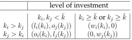
Table 1: Firm payoffs for different investment choices.
level of investment
ki, kj <k¯ ki ≥k¯orkj ≥k¯
ki > kj (li(ki), oj(kj)) (wi(ki),0)
kj > ki (oi(ki), lj(kj)) (0, wj(kj))
the contested segment but also by the captive consumers of firm j. We are interested in the set of Nash equilibria of this game. The structure of the game and frequencies of types are common knowledge. In reality, it is unlikely that a quality threshold such ask¯ determines with certainty which firm enters each consideration set. This simple modification of an otherwise standard setting allows us to represent the idea that in-vestment can be either incremental or radical, and that only a radical inin-vestment can make a firm visible to a consumer who is not yet aware of this firm’s product.6
Firm 1 and firm 2 simultaneously choose their investment levels. Firmireceives a payoff of
oi(ki) =αiProb(kj <¯k)−c(ki)
if it invests below the threshold (ki < ¯k) and less than its competitor (ki < kj). We
refer to the particular case where a firm does not investoi(0)as firm i’soutside option.
The outside option of firmidepends on the probability with which firmj chooses an
investment belowk¯, in which case captive consumers do not consider firmj’s invest-ment. Denote by
li(ki) = 1−αj −c(ki)
the payoff of firmiif it invests below the threshold (ki <k¯) and more than its
competi-tor (ki > kj). If firmiinvests above the thresholdki ≥ ¯k, captive consumers consider
both firms and the outside option of firmj drops to zero. In this case, firmicompetes for all segments of the market and earns at best a payoff
wi(ki) = 1−c(ki).
We assume that each relevant consumer segment is shared equally by both firms in case of a tie. If at least one of the two firms invests ¯k or more, the market becomes a monopoly because the highest quality firm then enters the consideration set of all con-sumers. Thus, for investments above¯k, the market becomes a winner-take-all market. We use this notation to summarize the corresponding payoffs for all combinations of investments in table 1.
2.2
Properties
We now derive some general properties of the equilibrium investments. The game faced by the two firms resembles an all-pay auction where the bids are given by the investment levels and prizes are given by the market shares. If the investment of a firm exceeds the threshold¯k, the market share of the winning firm increases discontin-uously as compared to a winning bid just below the threshold because at this point the investment is just high enough to attract the competitor’s captive segment in addition to the contested segment.
We first define the maximum possible level of investment at equilibrium as solving
c(kmax) = 1. It is never a best response for either firm to provide an investment greater
thankmax because the cost would then exceed the highest possible revenue. As can be
expected from the literature, the game does not have a pure-strategy equilibrium. The intuition is that it is profitable to marginally outbid any deterministic investment of the competitor because this only marginally increases costs but ensures winning the entire market.
Lemma 1. The game does not have an equilibrium in pure strategies.
Furthermore, even if the mixed strategies may contain mass points in equilibrium, these cannot be at the same investment levels for both firms. The intuition is that mass points in one firm’s investment strategy imply that the expected profit of the other firm from certain investment levels changes discretely at the respective investment level and overbidding is profitable.
Lemma 2. In equilibrium, at most one firm’s investment strategy has a mass point at any
given investment level.
We continue to show that apart from any mass points, the densities of both firms equilibrium investment strategies coincide.
Lemma 3. There exists 0< δ < k¯andK < k¯ max such that the densities of both firms’
equi-librium investment strategies are continuous and identical on the intervals(0, δ)and(¯k,K¯).
This result develops from the standard idea that the support of the equilibrium mixed strategy in an all-pay auction is connected and the density of equilibrium in-vestments over this interval is constant and is identical across contestants. The dif-ference with the existing literature comes from the possibility that the support of the investment strategy consists of two disconnected intervals. This results is driven by the discontinuity in the prize of winning at the threshold ¯k. For investments below
¯
This tradeoff between marginally overbidding and bidding exactly ¯k induces an
en-dogenous gap between the highest “low intensity” investmentδand the lowest “high
intensity” investment¯k.
Finally, we show that the equilibrium investment strategies of both firms admit mass points only at zero and at the threshold beyond which the consideration of cap-tive consumers is reached.
Lemma 4. If a firm bids a level of investment k with strictly positive probability, then k ∈ {0,¯k}.
The intuition behind this property is the following. Each firm generally prefers bidding marginally above k0 to bidding marginally below k0 if the competitor invests
k0 with strictly positive probability (see Lemma 1 and 2). Therefore, any investmentk0
that is chosen with a strictly positive probability in equilibrium must be at the lower bound of an interval of investments in the support of the mixed strategy. By Lemma 3, this implies that only investments of0ork¯can be chosen with strictly positive proba-bility.
A corollary of the above results it that as long as the other firm invests belowk¯with strictly positive probability, a firm has a positive reservation utility, from not providing any investment at all. The reservation utility is equal to the utility from the share of captive consumers multiplied by the probability that the competitor chooses an invest-ment below ¯k: o1(0) = Prob(k2 < ¯k)α1 for firm 1 ando2(0) = Prob(k1 < ¯k)α2 for firm
2. This implies that firms do not choose investments up to the level at which they just break even. Instead at the maximum investment, the expected profit conditional on this investment is equal to the reservation utility in form of the expected profit from not investing at all.
3
Equilibrium
We now characterize the equilibrium of the game for different levels of the threshold
¯
k. Let us assume without loss of generality that firm 1 enjoys a larger captive segment than firm 2, α1 > α2. We are looking for closed-form equilibrium solutions and focus
on the linear cost functionc(ki) =cki.
either firm to attract the competitor’s captive consumers. Thus, both firms only choose
investments below ¯kand compete for the contested segment only (Proposition 3). We
now turn to the analysis of these separate cases.
Consider first the case where the threshold is low, specifically,¯k < 1 c
α12+α21
1−α2 . Then,
it is relatively easy to enter the consideration set of consumers in the competitor’s captive segment. Moreover, both firms are in principle willing to choose investments high enough to do so. We show that in equilibrium both firms randomize over two disconnected intervals, one below and one above the thresholdk¯. In this equilibrium, firm 1 chooses to invest nothing with strictly positive probability because its larger share of captive consumers makes it compete less aggressively.
Proposition 1. If ¯k < 1cα12+α21
α12+α1 = ¯kl there exists a unique equilibrium in which both firms
randomize uniformly over two disconnected intervals: a lower interval (0, δ] and an upper interval(¯k,1
c −¯k α1
1−α2)whereδ = ¯k
(1−α1)α12
α12+α21
<k¯. The cumulative distribution functions are given by
F1(k) = c
1−α1−α2k+
c(α1−α2)¯k
(1−α1−α2+α21) ifk∈[0, δ]
c(1−α2)¯k
1−α1−α2+α21 if
δ < k≤k¯ ck+ c(1−α1)α1¯k
1−α1−α2+α21 if
¯
k < k ≤K
1 ifk > K
F2(k) =
k1−αc
1−α2 ifk∈(0, δ]
c(1−α1)¯k
1−α1−α2+α21 ifδ < k <
¯
k ck+ c(1−α1)α1¯k
1−α1−α2+α21 if
¯
k≤k ≤K
1 ifk > K
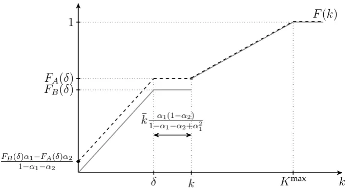
The cumulative distribution functions that characterize this equilibrium are such that, (i) at any interior point of both interval, both firms investment strategies have the same density and (ii) both firms investment strategies exhibit higher density on a given investment in the lower interval than in the upper interval. Moreover, firm 2 invests exactly ¯k with strictly positive probability, while firm 1 invests exactly 0with strictly positive probability. We represent the equilibrium strategies in Figure 1 and derive the following results with respect to profit and market leadership.
Corollary 1. In the equilibrium characterized by Proposition 1, firm 2 invests more in expec-tation and becomes a market leader with higher probability than firm 1. Both firms make an expected profit ofΠ =F2(δ)α1 =F1(δ)α2 >0.
FB(δ)α1−FA(δ)α2
1−α1−α2
1
FB(δ)
FA(δ)
δ k¯ Kmax k F(k)
¯
k α1(1−α2)
[image:11.595.75.423.68.254.2]1−α1−α2+α21
Figure 1: Proposition 1: Cumulative distribution functions if ¯k < 1c1−α1−α2+α21
1−α2 .
¯
K =
1 c−k¯
1−α1
1−α1−α2+α21. Dashed: firm 1, Gray solid: firm 2.
contested segment as well as the competitor’s captive segment in case of winning. Competition is however never perfect and both firms always make a strictly positive profit in equilibrium. This results from the fact that they can rely on the competitor being less aggressive with positive probability. In such a case the captive consumers remain unaware of the competitor’s offer and thus buy from the unique firm in their consideration set, even if this firm did not invest in its quality.
Both firms’ strategies are symmetric, except for the level of investments that they play with strictly positive probability. For each strictly positive investment below the threshold beyond which captive consumers come into play, it must hold that
f1(k) = f2(k) =
c α12
.
(1)
This is, by overbidding at a marginal costc, a firm increases its probability of winning the share α12 of indifferent consumers by αc12, so that the marginal benefit of
overbid-ding is also equal tocand the firm is indifferent between all levels of investment in the support. In the range of investments that attract also captive consumers, it must hold that
f1(k) =f2(k) =c.
(2)
This is because, for investments above¯k, having the highest investment is rewarded by serving the entire market of size 1, including all captive consumers and the contested
segment. The marginal benefit of overbidding must therefore equal the cost c. The
preceding arguments imply that the slopes of the cumulative distribution functionsFi
A consequence of these equilibrium investment strategies is that firm 2, having the smallest segment of captive consumers, invests more aggressively and becomes a market leader more often in expectation. This is not simply a curiosity deriving from the mixed strategy equilibrium but results from the larger captive segment making firm 1 more complacent. We find qualitatively similar results in an environment where investments have probabilistic returns in terms of market size and the equilibrium is in pure strategies (see Appendix B for details).
For the parameter values corresponding to Proposition 1, both firms make the same expected profit, even if firm 1 appears to be the favored one due to its larger captive segment. To understand the logic, it is helpful to consider the problem of firm 1: to maximize its profit, it must be the case that no “obvious” overbidding strategy is avail-able to firm 2. Hence, firm 1 wants to make firm 2 indifferent between all options in the support of the mixed strategy investment. In order to do so, firm 2 must believe that there is a sufficiently high probabilityP0 that firm 1 invest some amount belowk¯. Similarly, firm 2 wants firm 1 to be indifferent between all options in the support of the mixed strategy investment. For firm 1 to be indifferent between investments above and below k¯, it must believe that firm 2 invests some amount below k¯ with a sufficiently high probabilityP00. However, asα1 > α2 and expected profits are determined by the
outside options of both firms, E[Π1] = o1(0) = α1P00 = α2P0 = o2(0) = E[Π2], it must
hold thatP00 < P0. Thus, the mixed strategy of firm 1 must be less aggressive than that of firm 2 in order to make firm 2 indifferent between low and high investments. Firm 1 is thus trapped into less aggressive behavior by firm 2’s small captive segment.
At equilibrium, by definition, both firm 1 and firm 2 are indifferent between all investment levels in the support of the mixed strategy. Moreover, even if one of the two firms could commit ex-ante to a mixed strategy (using a randomization device), the one that would maximize each firm’s expected surplus is the equilibrium one.
This result implies that the larger (dominant) firm is less likely to invest sufficient amounts into quality to enter all consumers’ consideration sets. Instead, it counts on its large captive segment remaining unaware of the competitor and abstains from com-petition for the competitor’s small captive segment.
Consider second the case, where the threshold is sufficiently high for firm 1 not to find it worthwhile to attract the consideration of firm 2’s captive share but firm 2 may still want to attract firm 1’s captive segment. This asymmetry arises because firm 1 is more content with its larger captive segment, and 2 is more eager to escape its initially inferior market position.
Proposition 2. Ifk¯l <¯k < α12c+α1 = ¯kh, there exists a unique equilibrium in which both firms
randomize uniformly over a single interval(0, δ), whereδ= ¯k−α1
The cumulative distribution functions are given by
F1(k) =
c α12k+
1−α2−ck¯
α12 ifk ∈[0, δ]
1 ifk ≥δ
F2(k) =
c
α12k ifk ∈(0, δ]
c
α12k ifδ ≤k≤
¯
k
1 ifk ≥¯k
The distribution functions are such that, at any point of the interval, both firms in-vest with the same density. Moreover, Firm 2 inin-vests exactly ¯k with strictly positive probability, while Firm 1 invests exactly0with strictly positive probability. We imme-diately obtain the following corollary regarding market outcomes.
Corollary 2. In the equilibrium characterized by Proposition 2, firm2invests more in expecta-tion than firm 1 and becomes a market leader more often. The expected profit of firm2is1−c¯k
and the expected profit of firm1isα1 >1−ck¯.
The result from Proposition 2 is similar to that from Proposition 1 but here it is too costly for firm 1 to attract the captive segment of firm 2. Thus, firm 1 does not choose investments equal to or abovek¯at all. As in the preceding arguments for investments belowk¯, it is still the case that both density functions satisfy
f1(k) = f2(k) =
c α12
.
(3)
At or above ¯k, only firm 2 invests. As it does not face competition at or above k¯, firm 2 chooses an investment exactly equal tok¯ with strictly positive probability and does never choose any strictly higher investment. This level is sufficient not only to
outbid firm 1 but to also attract firm 1’s captive segment with certainty. Firm 1 in
contrast decides not to invest at all with a strictly positive probability and otherwise randomizes over relatively low investment levels.
Corollary 2 shows that, in this equilibrium, expected profits of both firms differ. Firm 1 benefits from its larger base, invests less and makes a higher expected profit than firm 2. The asymmetry in this equilibrium is twofold: firm 2 invests more aggres-sively and wins the market more often, but firm 1 actually makes the highest profit in expectation.
differently sized captive segments, they behave identically and end up dominating the market with equal probability.
Proposition 3. If k >¯ ¯kh, there exists a unique equilibrium in which both firms randomize
uniformly over a single interval[0,α12
c ].
The cumulative distribution functions are given by:
Fi(k) =
c
α12k for allk ∈[0,
α12
c ]
1 fork ≥ α12
c
fori= 1,2
The distribution functions are such that, at any point, both firms invest with the same density. No firm invest at any point with strictly positive probability. No firm ever chooses an investment that would attract the consideration of the competitor’s captive segment. Therefore, expected payoffs must equal the firms’ outside options and market leadership is reached with equal probability.
Corollary 3. In the equilibrium characterized by Proposition 3, both firms invest the same amount in expectation and become a market leader with equal probability. The expected profit of firm2isα2 and the expected profit of firm1isα1 > α2.
While it is obvious that competition for the entire population is not profitable for
¯
k > kmax = 1c, it is the case that¯kh < kmax. A priori, high investments can be profitable
fork¯h < ¯k < kmax if the success probability is high enough. However, in equilibrium
this is not the case so that neither firm chooses investments equal to or abovek¯. As a consequence,limε→0F(¯k−ε) = 1and captive consumers do not consider the
competi-tor’s offer.
Having characterized these three equilibria, we now establish that this characteri-zation is complete.
Proposition 4. The equilibrium of the investment game is unique and is characterized by
Proposition 1, 2 or 3 for low, intermediate, and high levels of¯k, respectively.
The uniqueness result closely relates to the equilibrium properties outlined in Lem-mas 1 to 4. An equilibrium can either be a mixed strategy over two intervals or over a single connected interval. Proposition 1 characterizes an equilibrium over two inter-vals. Propositions 2 and 3 characterize two candidate equilibria over a single interval. The formal proof shows that for neither of the three cases, an alternative equilibrium exists. As the existence condition the three existing equilibria are mutually exclusive, the equilibrium is indeed unique. This equilibrium is “stable” in the sense that best responses to any small perturbation to the equilibrium probabilities would bring the game back to equilibrium.7
7Consider a level of investment k0 < ¯kthat is chosen by both firms with densityf(k0) = c α12 in
4
Implications
In this section, we discuss the major policy implications of our equilibrium results, mostly focusing on the case where both firms are in the position of competing for the whole market, described in Proposition 1. First, we show that the size of the contested segment, α12has a non-trivial effect on competition. Second, the size of the dominant
firm’s captive segment α1 has a non-monotonic effect on both firms’ levels of
invest-ment. Third, we study the effect of changing the difficulty of reaching the competitor’s captive consumers’ consideration sets captured by our threshold¯k.
4.1
The share of consumers initially observing both firms has an
am-biguous impact on investment
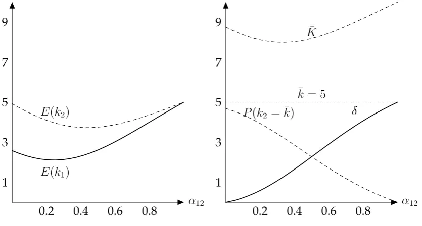
The marginal effect of increasing the share of ante indifferent consumers on ex-pected investments is ambiguous and depends on the conjunction of three effects, that we illustrate in Figure 2 for parameter values corresponding to Proposition 1. The ag-gregate effect of α12 on expected investments is shown in the panel on the left-hand
side (Figure 2a). The expected investment of the firm with the smallest captive seg-ment, firm 2, initially decreases with α12, and only reaches its initial level when the
share of the contested segment approaches1. For the firm with the larger captive seg-ment, firm 1, the effect of an increase in the contested segment is also negative in the beginning but becomes positive asα12surpasses 12.
We plot the influence of the share of the contested segment α12 on three crucial
aspects of the firms’ investment strategies on the right-hand side (Figure 2b). First, δ, the upper bound of the lower part of the investment strategies’ support, monotonically increases to ¯k as the share of the contested segment goes to 1. This effect is driven by the fact that investing at or above k¯ becomes increasingly irrelevant to a firm as the captive segment of the competitor vanishes.
Second,α12has the opposite effect on the probability that firm 2 chooses the highest
investment level. The probabilityP(k2 = ¯k)of firm 2 investing exactly ¯kdecreases as
α12 increases because its investments are spread over a larger interval with a higher
δ. When investments are more spread out, less probability mass can be allocated to
¯
k. AsP(k2 = ¯k) = P(k1 = 0), this implies that the probability of firm 1 not investing
at all also decreases. Consequently, an increase in the share of contested consumers makes the firm with a smaller (larger) captive segment invest less (more) aggressively.
Then, firm 2 would want to put more weight on the investment level marginally abovek0, as marginally outbidding an investment ofk0 would yield an expected benefit ofφα12 > c. This change in firm 2’s
α12
0.8 0.6
0.4 0.2
1 3 5 7 9
E(k1)
E(k2)
(a) Expected investments in equilibrium.
α12
0.8 0.6
0.4 0.2
1 3 5 7 9
δ P(k2 = ¯k)
¯
K
¯
k = 5
[image:16.595.76.494.69.293.2](b) Elements of equilibrium bidding strategies.
Figure 2: Comparative statics with respect to the share of ex-ante indifferent consumers
α12 within the equilibrium of Proposition 1. Illustration with c = 0.1,k¯ = 5 andα1 =
3α2.
This results is driven by the fact that the absolute level of asymmetry between the two firms’ captive segments shrinks as the contested segment becomes larger.
Third, the maximum bidK¯ initially decreases withα12because the presence of more
contested consumers reduces the additional expected profit from investing at or above
¯
k. It then increases when competition for the growing contested segment becomes
fiercer.
4.2
The share of captive consumers of the dominant firm has a
non-monotonic effect on both firms’ investments
While the above discussion is useful to disentangle the different effects, it does not provide a tractable result, as further assumptions are needed on how the different sub-groups of captive consumers evolve if the contested segment increases. In this section, we focus on the perhaps most policy-relevant question of a dominant firm using its market power to increase the share of its own captive consumers, who initially observe only this firm’s product but are unaware of the competitor.
We make the assumption that the smallest firm has no captive consumers (α2 =
0) and study the impact of an increase in α1. We further assume the threshold ¯k is
sufficiently small for the equilibrium to be characterized by Proposition 1.
Proposition 5. The share of captive consumers of firm 1 has a non-monotonic effect on both firms’ investment.An increase in α1 has a negative effect forα1 small and a positive effect for
When the share of firm 1’s captive consumers, who initially consider only the prod-uct of the dominant firm 1, increases, this has two effects. First, we observe an anti-competitive effect because the dominant firm 1 invests less asα1increases. The reason
is that firm 1’s outside option increase, that is its payoff when not investing at all. As investments are strategic complements, firm 2 also invests less. Second, there is a pro-competitive effect because an increasing share of captive consumers implies that an increasing share of the market can be reached only by investing above the thresh-old. Thus, these high investments become more profitable for the underdog firm 2 as
α1 increases, and due to complementarity both firms choose these investments more
often.
The first effect dominates when few consumers are captive to firm 1, whereas the second effect dominates when already most consumers are captive to firm 1. As long as we stay in the realm of Proposition 1 where both firms are in position to compete, when the dominant firm becomes too dominant, it leaves no other option to the other firm but to compete very aggressively for the entire market. Again, investments are strategic complements so that this results in both firms investing more. When the dominant firm 1 is not too dominant, however, a higher share of captive consumers makes competition softer by segmenting the market.
4.3
Comparing the different equilibria
We now relax the assumption that the threshold¯kis low enough for the equilibrium in proposition 1 to hold and that α2 = 0, and compare the three possible equilibria. We
illustrate the effect of¯kon expected investments in Figure 3. The vertical dotted lines represent the values ofk¯that delimit the zones corresponding to Propositions 1 to 3.
When the investment threshold k¯ is small but strictly positive (part (i) of Figure 3, Proposition 1) both firms compete for the captive segment of their competitor with positive probability but not with certainty. Whenever both firms choose investments below¯k, competition is softened because it is restricted to the contested segment. Both firms can then serve their captive segments even at an investment of zero. As a con-sequence, both firms include zero investment in their investment strategy and make strictly positive profits in expectation. Competition is dampened if ¯k increases and firm 1 puts increasingly more mass on not investing at all. As a result, bothE(k1)and
E(k2)decrease with¯k, and the gap between the two increases with¯k. Thus, while part
(i) applies, both firms invest less in quality as it gets harder to enter the consideration set of the competitor’s captive consumers.
¯
k
12 11 10 9 8 7 6 5 4 3 2 1 1 2 3 4 5
E(k1)
E(k2)
¯
kl= 1c α12+α21
α12+α1
¯
kh = α12+cα1
(ii) (iii)
[image:18.595.139.456.72.299.2](i)
Figure 3: Expected equilibrium investment in the equilibria corresponding to Propo-sitions 1 in part (i), 2 in (ii), and 3 in (iii). Illustration with α1 = 0.4, α2 = 0.1 and
c= 0.1.
for these values, and as opposed to Proposition 1, the probability mass allocated to boundary points,P(k1 = 0) = P(k2 = ¯k), decreases with the threshold¯k. This implies
that the investment strategies of firms become more and more symmetric, whereas the profits become more and more asymmetric as the profit effect of the asymmetric captive segments kicks in.
Whenk¯ reaches the level at which firms decide to only compete for ex-ante indif-ferent consumers (part (iii) of Figure 3, Proposition 3), the expected investments in both types of equilibrium are the same and the expected level of investment remains constant for further increases in k¯. Firms compete only for the contested segment of consumers who anyway consider both firms. Therefore, investment behavior is inde-pendent of¯k.
5
Conclusion
of these captive segments induces asymmetries in the probabilities of one or the other firm dominating the market. The reason is that the outside option of serving only its own captive segment in a shared market is less attractive for a firm with a small captive segment than it is for the competitor with a larger one.
The effect of the share of captive consumers on total expected investments is non-monotone: if the underdog has sufficient resources to target the whole market, a higher share of captive consumers of the dominant firm may lead to higher investments. This may well have been the case for Internet Explorer competing with Google Chrome. When Microsoft chose to breach its 2009 promise to make Windows users aware of the existence of competing browsers to Internet Explorer, Google was already big enough to compete aggressively, and eventually overtook most of the market before regulators forced Microsoft to place Google Chrome such that it would enter the consideration set of Windows users. Hence, a key question for a regulator is to identify whether a competitor with the potential to overtake the whole market exists. Facing a weak underdog, a regulator may do well to prevent the dominant firm from keeping con-sumers unaware of alternatives to its products. Facing a strong underdog, the case is much more balanced.
References
ARBATSKAYA, M. (2007). Ordered search.The RAND Journal of Economics, 38(1), 119–
126.
ARMSTRONG, M. and VICKERS, J. (2018). Patterns of competition with captive cus-tomers.
—, — and ZHOU, J. (2009). Prominence and consumer search. The RAND Journal of
Economics,40(2), 209–233.
BAYE, M. R., KOVENOCK, D. and DE VRIES, C. G. (1996). The all-pay auction with
complete information.Economic Theory,8(2), 291–305.
BURDETT, K. and JUDD, K. L. (1983). Equilibrium price dispersion.Econometrica: Jour-nal of the Econometric Society, pp. 955–969.
DE CORNIERE, A. and TAYLOR, G. (2019). A model of biased intermediation. RAND
Journal of Economics, p. forthcoming.
FARRELL, J. and KLEMPERER, P. (2007). Coordination and lock-in: Competition with
— and SHAPIRO, C. (1988). Dynamic competition with switching costs. The RAND Journal of Economics, pp. 123–137.
FUDENBERG, D. and TIROLE, J. (2000). Customer poaching and brand switching. RAND Journal of Economics, pp. 634–657.
GEHRIG, T. and STENBACKA, R. (2004). Differentiation-induced switching costs and poaching.Journal of Economics & Management Strategy,13(4), 635–655.
JIA, H. (2008). A stochastic derivation of the ratio form of contest success functions.
Public Choice,135(3-4), 125–130.
KLEMPERER, P. (1987). Markets with consumer switching costs. The Quarterly Journal of Economics, pp. 375–394.
MOLDOVANU, B. and SELA, A. (2001). The optimal allocation of prizes in contests. American Economic Review, pp. 542–558.
ROBERSON, B. (2006). The Colonel Blotto game.Economic Theory,29(1), 1–24.
SIEGEL, R. (2009). All-pay contests.Econometrica,77(1), 71–92.
Appendix
A
Proofs
Proof of Lemma 1
Proof. The proof is by contradiction. Suppose there is pure strategy equilibrium in which firms1and2choose investmentsk1, k2 < kmaxwith certainty. Suppose first that
k1 = k2. Obviously, each firm could profitably deviate to marginally overbidding the
other as this would only marginally increase cost but discretely increases the chance of winning. Thus, this cannot be an equilibrium. Suppose insteadk1 < k2. We distinguish
two cases. Ifk2 ≥¯k, firm 1 can profitably deviate to investing just marginally abovek2
which would imply winning the entire market with certainty and byk2 < kmax would
yield a positive profit. Now consider the casek2 <k¯. This can only be an equilibrium
if firm 1 chooses k1 = 0 because it looses in any case. But then, firm 2 would want
to just marginally overbid 0 which could in turn be profitably outbid by firm 1. Thus, these investments do not constitute an equilibrium either. The analogous arguments
hold if we exchange subscripts 1and 2. Therefore, the equilibrium must be in mixed
strategies.
Proof of Lemma 2
Proof. The proof is by contradiction. Suppose firm1 invests according to an equilib-rium investment strategy F1 and as part of it chooses k1 = k0 with strictly positive
probability,P1(k0) >0. Suppose further that also firm 2 choosesk0 with positive
prob-ability, i.e., P2(k0) >0is part of firm 2’s equilibrium strategyF2. Denote byE[Π2]the
expected profit of firm 2 given this strategy. Note that firm 2 can discretely increase its expected profit by switching to a mixed strategyF20 that differs fromF2 only in that
firm 2 reallocates probability mass from k0 to an investment of k2 = k0 + for any
> 0small enough. Thus, both firms will not allocate positive probability to the same investment.
Proof of Lemma 3
Proof. (i) We first show that, if there is a gap in the support of the mixed strategy
of a firm, the gap must be an interval containing ¯k. Suppose there is a gap
[k0, k00] in the support of firm i0s strategy between with k0, k00 ∈ (0,k¯), k0 < k00, and Fi(k0) = Fi(k00). Note that firm j then strictly prefers investing k0 over
for the lower investment. Thus, firm j prefers to marginally overbid firm i at
k0 over any higher investment and in particular over investing k00. This in turn implies that firmialso strictly prefers to invest marginally above firmj’s invest-ment over investing k00 because k00 is more expensive but does not increase the chance of winning. Thus, the condition that a firms has the same expected profit over the support of her mixed strategy would be violated. The same reasoning applies to any pairk0, k00 >¯k. Thus, if there is a gap, it must be the case thatk0 <¯k
andk00≥k¯.
(ii) It follows that any gap must have as an upper boundk¯. Else, following the same logic as above, a firm would strictly prefer biddingk¯over somek00 >k¯. Hence, if there is a gap, it must be in some interval[δ,k¯].
(iii) The fact that firms randomize over the same intervals is a standard property: if an investmentkis part of only one firm’s mixed strategy support, this firm would be better off investing less (at the top of the other firm’s support). The fact that the bottom of the lower investment support is zero is also standard: else investing zero with strictly positive probability would be a profitable deviation.
Proof of Lemma 4
Proof. For a mass point to be an equilibrium strategy, it must satisfy two properties. First, by Lemma 2, a firm does not invest k with strictly positive probability in equi-librium ifk is in the support of the other firm’s strategy. Else, the other firm would be better off marginally outbiddingkthan bidding just below it. Second, the same holds if a value marginally below k is in the support of the other firm, for a similar reason. There needs to be a gap in the support of the mixed strategy of player ibelow an in-vestment k for firmi to investk with strictly positive probability in any equilibrium. This leaves only two possibilities: k = 0(as no one invests below0) andk = ¯k (if there is a gap in the support of the investment strategy of the other firm below¯k).
Proof of Proposition 1
Proof. We first construct the equilibrium, then verify that indeed neither firm has an incentive to deviate from the proposed investment strategy, and finally show that no other equilibrium exists.
Characterization: For every investment of firm 2below ¯k which is contained in the
arbi-trarily small):
(4) F2(k)α12+ lim
ε→0F2(¯k−ε)α1−ck = limε→0F2(¯k−ε)α1 ⇒ F2(k) =
c α12
k
and for every investment equal to or above¯k
(5) F2(k)−ck= lim
ε→0F2(¯k−ε)α1 ⇒ F2(k) =ck+ limε→0F2(¯k−ε)α1
If firm1 chooses zero with positive probability, firm 2’s mixed strategy must not contain an atom at zero. However, firm 2must also be indifferent between all invest-ment levels in the support of its equilibrium mixed strategy. Denote firm 2’s expected profit byE[Π2]. Then, for allk <k¯
F1(k)α12+ lim
ε→0F1(¯k−ε)α2−ck=E[Π2]
⇒ F1(k) =
c α12
k+E[Π2]−limε→0F1(¯k−ε)α2
α12
(6)
For every investment at k¯ or above having a lower investment than the competitor
implies also losing their share of captive consumers.
(7) F1(k)−ck=E[Π2] ⇒ F1(k) =ck+E[Π2]
From lines (4) to (7) it follows that firm 1’s and firm 2’s distribution functions have the same slopes. This is true in both the low and the high investment range. Since the slope is higher for investments below ¯kthan for investments above ¯k, there exists
δ ∈(0,k¯)such that for both firms
(8) F1(k) =F1(δ)andF2(k) = F2(δ)for allk ∈[δ,¯k)
and thereforelimε→0F1(¯k−ε) = F1(δ)andlimε→0F2(¯k−ε) =F2(δ).
Neither firm has an incentive to strictly exceed the maximum investment of the other. This would increase the cost but not the probability of winning. Thus, there exists a unique K such that F1(K) = F2(K) = 1and for all ε > 0, F1(K −ε) < 1and
F2(K −ε) < 1. Since the distribution functions of firms 1 and 2 also have identical
slopes fork≥k¯, the distribution functions of both firms are identical fork ≥¯k:
Combining Equations (5), (7), and (9) yieldsE[Π2] =F2(δ)α1. Starting with Line (6)
and plugging in yields fork <¯k
(10) F1(k) =
c α12
k+F2(δ)α1
α12
−F1(δ)α2
α12
.
We solve (10) forF2(δ)atk=δand obtain
F2(δ) =F1(δ)
α12+α2
α1
− c
α1
δ.
We plug in from line (4) and solve forF1(δ)to obtain
(11) F1(δ) = cδ
α1
α12(α12+α2)
+ 1
α12+α2
.
The flat part in the distribution functions (equation (8)) implies together with the different shares of captive consumers that firm2chooses an investment equal to¯kwith a positive probability while firm 1’s strategy has an atom at zero. Since the two firms cannot have an atom at the same investment level (Lemma 2), and since neither firm choosesδwith positive probability in equilibrium (Lemma 4), the distribution function of firm 1must be continuous inδandk¯. In addition, at¯kthe distribution functions of both firms take identical values. Thus, the following holds
(12) F1(δ) = F1(¯k) =F2(¯k)
We can rewrite (5) using (4) as
(13) F2(¯k) = ck¯+
c α12
δα1.
Taking line (12) and plugging in from line (11) on the left-hand side and from line (13) on the right-hand side, we arrive at
cδ
α1
α12(α12+α2)
+ 1
α12+α2
=c¯k+ c
α12
δα1
⇔ δ= ¯k α12(α12+α2) α12+α1−α1(α12+α2)
= ¯k(1−α1)α12 α12+α21
.
(14)
It is easily verified that
(1−α1)α12 < α12+α21 ⇒δ <¯k.
level chosen, we obtain the following condition
(15) cK +F2(δ)α1 = 1 ⇔cK = 1−
α1c
α12
δ = 1−α1c¯k
(1−α1)α12
α12(α12+α21)
whereδhas been derived in Equation (14). Rewriting (15) yields the maximum
invest-ment level
K = 1
c −α1
¯
k 1−α1 α12+α21
.
As by assumptionα1+α2+α12= 1, we replace in the above results to state
Propo-sition 1.
For the derivation of the maximum investment, we have assumedK > ¯k. This is indeed true if
(16) 1
c −α1
¯
k 1−α1 α12+α21
>k¯⇔¯k < 1 c
α12+α21
1−α2
.
Equilibrium verification: The above computations establish that both firms are
in-different between all levels of investment in their support such that it does not pay to reshuffle probability mass within interior investments. Hence, it suffices to show that there is no strictly profitable deviation for either firm to investments outside the sup-port or at the boundaries. Note that by construction no firm has an incentive to deviate to an investment in the gap or above K¯, as this would yield strictly lower expected profit. Note further that firm 1 would be strictly worse off to invest¯kwith strictly pos-itive probability than what she already gets by investing marginally abovek¯(as firm 2 invests exactlyk¯with strictly positive probability). The same holds for firm 2 investing exactly0, as it would get strictly lower profit then by investing just above0.
Uniqueness: By the above construction, the slopes of the distributions over the two
intervals and the value of δ are the only ones satisfying the condition of equal profit over the intervals. We also know from Lemmas 2 and 4 that the only other possibility in terms of a mass point satisfying the condition that both firms need to invest with total probability of 1would be to have firm 1 investingk¯with strictly positive probability and firm 2 investing0with strictly positive probability. However, in any equilibrium
over two intervals, with K¯ the upper bound of the upper interval, it must hold by
Lemma 3 that F1( ¯K) = F2( ¯K) = 1, the profit of both firms must be identical. This
does not hold ifα1 > α2, F2(0) > 0 and F1(0) = 0. Hence, Proposition characterizes
Proof of Corollary 1
Proof. Using the distribution functions from Proposition 1, we observe that F1(δ) >
F2(δ)so that firm 2 has a higher investment than firm 1 more often than the reverse.
We compute expected investments as
E[k1] = Z δ 0 c α12 xdx+ Z K ¯ k cxdx
= c(1−α1)2α12k¯2
2(α12+α21)
2 + 12c
(α12−α1((1+α1)ck−α¯ 1))2
c2(α 12+α21)
2 −¯k2
E[k2] = Z δ 0 c α12 xdx+ Z K ¯ k
cxdx+Prob(k2 = ¯k)¯k
= c(1−α1)2α12k¯2
2(α12+α21)
2 +
1 2c
(α12−α1((1+α1)ck−α¯ 1))2
c2(α 12+α21)
2 −¯k2
+c(α1−α2)¯k2
α12+α21
It is easily verified that E[k1] < E[k2]. By the properties of the mixed strategy
equi-librium, the expected profit of each firmi = 1,2equals its expected profit conditional on investing zero. This corresponds to its outside option oi(0) which is the value of
its captive segment multiplied with the probability of the competitor investing below
¯
k.
A.1
Proof of Proposition 2
Proof. We first construct the equilibrium and then verify that indeed neither firm has an incentive to deviate from the proposed investment strategy, and finally show that no other equilibrium exists.
Characterization: Suppose that both firms randomize over (0, δ)for someδ ∈ (0,¯k). Suppose further that firm1chooses zero with positive probability and firm2chooses
¯
k with positive probability. Finally, suppose that firm1chooses investments below or equal toδwith certainty (we verify this later), i.e.,F1(δ)whereas firm2also chooses¯k
such thatF2(δ)<1. We now derive the value forδ ∈(0,¯k).
As firm 1 invests only belowk¯, firm2could ensure profit1−c¯kby investingk¯with certainty. Thus, the distribution function of firm1must fulfill for allk ≤δ
(17) F1(k)α12+α2−ck= 1−c¯k ⇒F1(k) =
c α12
k+1−α2−c¯k
α12
By assumption k <¯ 1−α2
c and thus
1−α2−c¯k
α12 > 0. Note that choosing
¯
k also yields an expected profit equal to1−ck¯for firm2.
Firm 1obtains an expected profit equal to its outside option o1(0) which is given
F2(δ)α1. For the distribution function of firm 2and investments k ≤ δ the following
must hold:
F2(k)α12+F2(δ)α1−ck =F2(δ)α1 ⇔F2(k) =
c α12
k
The investment levelδis such that the distribution function of firm1just reaches 1 at this level
(18) c
α12
δ+ 1−α2 −c ¯
k α12
= 1⇔δ= ¯k−α1
c
Ifk <¯ 1−α2
c , thenδ < α12
c .
Finally, we derive the probability with which firm2choosesk¯.
Prob(k2 = ¯k) = 1−
c α12
δ = 1−1 + 1−α2
α12
− c
α12
¯
k = 1−α2
α12
− c
α12
¯
k
From line (17) also
Prob(k1 = 0) =
1−α2
α12
− c
α12
¯
k =Prob(k2 = ¯k)
By¯k < 1−α2
c , it holds that Prob(k2 = ¯k)>0. Moreover,
α12 >0⇒α12+α2 > α2 ⇒(1−α1)2 > α2(1−α1)⇒α12+α21 > α1−α1α2
⇒ α12+α
2 1
1−α2
> α1
and therefore
¯
k > 1 c
α12+α21
1−α2
⇒¯k > α1 c
so thatδ <¯k. Byk >¯ 1cα12+α21
1−α2 firm1does indeed not want to deviate to choosing
¯
k:
¯
k > 1 c
α12+α21
1−α2 ⇒c
¯
k(α12+α1)> α12+α21 ⇔ − α2
1
α12 +
c α12
¯
kα1 >1−ck¯⇔F2(δ)α1 >1−ck¯
Equilibrium verification: From the above derivations, both firms are indifferent
Uniqueness: By the above construction, the cumulative distribution functions and the value of δ are the only ones satisfying the indifference condition for randomiza-tion of investments over a single connected interval. We also know from Lemmas 2 4 that the only other possibility in terms of mass points satisfying the condition that both firms need to invest with total probability of 1would be to have firm 1 invest ¯k
with strictly positive probability and firm 2 invest 0with strictly positive probability. However, for such a mixed strategy to be an equilibrium it must also be true that firm 1 is indifferent between investing just above0and exactly¯k,
α1+F2(0) = 1−ck,¯
and that firm 2 weakly prefers to invest0over investingk¯,
F1(δ)α2 ≥1−c¯k.
Asα1 > α2, F1(δ) < 1 andF2(0) > 0, this leads to a contradiction. Hence, the above
equilibrium is the unique one where both firms randomized over the same connected interval, when the total probability mass allocated belowδ(remember there is only one possible slope for the distribution at equilibrium) is strictly below 1. Note further that there cannot be an equilibrium where firms randomize over two disconnected intervals as the one described in Proposition 1 is the only one that exists but the condition on¯k
is not fulfilled here. Thus, the equilibrium we characterized here is unique for the set range ofk¯.
Proof of Corollary 2
Proof. Using the distribution functions from Proposition 2, we observe that F1(δ) >
F2(δ), and we compute expected investments as
E[k1] = Z δ
0
c α12
xdx= c(
α1
c −¯k) 2
2α12
E[k2] = Z δ
0
c α12
xdx+Prob(k2 = ¯k)¯k =
c(α1
c −k¯) 2
2α12
+ ¯kα1+α12−c
¯
k α12
where obviouslyE[k1]< E[k2].
By the properties of the mixed strategy equilibrium, the expected profit of each firm
i = 1,2 equals its expected profit conditional on investing zero which is its outside option oi(0) which is given by its captive segment multiplied with the probability of
A.2
Proof of Proposition 3
Proof. Letk >¯ 1−α2
c . We first construct the equilibrium, verify that neither firm has an
incentive to deviate, and finally show that no other equilibrium exists.
Characterization: Suppose that neither firm chooses an investment high enough to
steal captive consumers from its competitor. The outside option of firm i = 1,2 is to keep its captive segment and receive a profit of oi(0) = αi. The prize of winning is
then the value of additionally attracting the contested segment α12. This observation
implies that both firms are symmetric at the margin. Moreover, the captive segments can be disregarded since they are not at stake. Both firms compete until their expected profits from competition are zero, in which case their expected profit is determined only by their captive segment. Thus, in equilibrium, the following must hold for all
ki <k¯fori= 1,2andj 6=i:
(19) Fj(ki)α12−cki = 0⇔Fj(ki) =
c α12
ki.
As the distribution function of investments cannot exceed 1, both firms random-ize continuously over [0,α12
c ]and do not invest any higher amounts. The cumulative
distribution function is as follows for firmi= 1,2:
Fi(k) =
c
α12k for allk ∈[0,
α12
c ]
1 fork ≥ α12
c
Each firm must be indifferent at equilibrium between all investments in [0,α12
c ], and
none of the two firms chooses zero with strictly positive probability because this would not be consistent with the indifference condition in (19). The expected payoff of firm 1 and 2 is equal to its outside option, E[Π1] = o1(0) = α1 and E[Π2] = o2(0) = α2,
respectively.
Equilibrium verification: By the above, both firms are indifferent between all levels
of investment in their support by construction. Hence, it suffices to show that there is no strictly profitable deviation for either firm. Suppose firmiconsidered deviating to an investment at ¯k, sufficient to capture the entire population. Then, firmi would make an expected profit of F(α12
c ) −c¯k = 1− ck <¯ 1 −(1 −α2) = α2 < α1 such
that this deviation is not profitable for firm i = 1,2. As a consequence, no investment level at or above k¯ forms part of the equilibrium mixed strategy. We also know that
any investment between α12
c and ¯kwould yield strictly lower profit, hence there is no
Uniqueness: We have shown above that the slopes of the distributions and the value of δas specified in the equilibrium characterization are the unique ones satisfy-ing the condition of equal profit for randomization over a ssatisfy-ingle connected interval. Hence, the above equilibrium is the unique one on a single interval when the total probability mass allocated below δ is equal to 1. Note further that there cannot be an equilibrium where firms randomize over two disconnected intervals as the one de-scribed in Proposition 1 is the only one that exists but the condition on¯kis not fulfilled here. According to Lemmas 1 to 4, no further equilibrium types are admissible. Thus, the equilibrium we characterized here is unique for the set range of¯k.
Proof of Corollary 3
Proof. Using the distribution functions from Proposition 3, the expected investment in equilibrium equals
E[ki] = Z α12c
0
c α12
xdx= 1 2
α12
c fori= 1,2
per firm. In total, the two firms invest α12
c . Since equilibrium mixed strategies and
investments are identical, both firms have the same probability of winning of 1
2. The
expected profit of each firm equals its expected profit conditional on investing zero which is the value of its captive segment.
A.3
Proof of Proposition 4
Proof. Propositions 2 and 3 each characterized an equilibrium that is unique for the
range of k¯ to which the respective proposition applies. The proof is completed by
noting that the ranges of k¯ given in Propositions 1 to 3 constitute a partition of the admissible range for¯k.
A.4
Proof of Proposition 5
Using the investment levels found in Proposition 1, replacingα2by0andα12by1−α1
and taking the derivative with respect toα1 we find
dE(k1)
dα1
= ¯
k(α1(4 +α1c¯k)−c¯k−2)
2((α1−1)α1+ 1)2
and
dE(k2)
dα1
= ¯
k(α1(4−α1c¯k)−c¯k−2)
2((α1−1)α1+ 1)2
Takingα1 →0we find
lim
α1→0
dE(k1)
dα1
=−1 2 ¯
k(ck¯+ 2)<0
and
lim
α1→0
dE(k2)
dα1
=−1 2 ¯
k(2−ck¯)<0,
as we have assumedck <¯ 1. Similarly, we find
lim
α1→1
dE(k1)
dα1
= lim
α1→1
dE(k2)
dα1
= ¯k >1.
B
Probabilistic setting
In this section, we show that the fact that investment is deterministic with a discrete thresholdk¯is not crucial to our results. Consider two firms, 1and 2choosing a level of investment ei, withi ∈ {1,2}, at costc(ei)with c0 > 0, c00 > 0and c(0) = 0. Firms
compete for consumers from a population of mass one. This population consists of three types of consumers,t1, t2, andtu. Typest1 andt2occur with frequencyα1andα2,
respectively, in the population and the remaining part are of typetu,α12. The structure
of the game and frequencies of types are common knowledge.
Different from the main part of the text, we assume captive consumers of firm i
(types t1 andt2) bear a switching cost¯k if they join the other firm. Hence, the utility
of a consumer visiting a firmiis equal toei, minus the switching cost when it applies.
Consumers of typetuare ex ante undecided and do not experience switching costs.
Suppose all types of customers intend to join the firm that maximizes their utility but may make mistakes and join the “wrong” firm. We employ the commonly used ratio-form contest success function which imposes that the probability of choosing one firm over the other equals its share in total investments.8
The ex-ante indifferent consumers choose firmiwith a probability
(20) pitu(ei, ej) =
ei
ei+ej
.
The captive consumers of typetichoose the firmiwith a probability
(21) pit
i(ei, ej) =
ei+ ¯k
ei+ej+ ¯k
.
8Jia (2008) shows how such a contest success function can be derived from a model where the
Therefore, the captive consumers of typetj choose firmiwith a probability
(22) pitj(ei, ej) = 1−pii(ei, ej) =
ei
ei+ej+ ¯k
.
Firm1chooses the level of investment that maximizes her expected profit
(23) E(Π1) =α12p1tu(e1, e2) +α1p
1
t1(e1, e2) +α2p
1
t2(e1, e2)−c(e1).
Solving the first-order condition of the profit maximization with respect toeayields
(24) c0(e1) =
α12e2
(e1+e2)2
+ e2(α1+α2) +α2 ¯
k
(e1+e2+ ¯k)2
.
Solving the same way for firmbyields
(25) c0(e2) =
α12e1
(e1+e2)2
+ e1(α1+α2) +α1 ¯
k
(e1+e2+ ¯k)2
.
We immediately observe that:
(i) The equilibrium level of investment decreases in the cost-efficiency (the c func-tion).
(ii) The firm that invests the most in equilibrium is the firm with the smallest captive segment.