Development and application of capillary
electrochromatography using modular instrumentation.
KING, Adrian.
Available from Sheffield Hallam University Research Archive (SHURA) at:
http://shura.shu.ac.uk/19917/
This document is the author deposited version. You are advised to consult the
publisher's version if you wish to cite from it.
Published version
KING, Adrian. (2001). Development and application of capillary
electrochromatography using modular instrumentation. Doctoral, Sheffield Hallam
University (United Kingdom)..
Copyright and re-use policy
LCrtmiwu ocm ht CITY CAMPUS, POND STREET,
SHEFFIELD, SI 1WB.
1 0 1 7 1 5 6 2 9 8
ProQuest Number: 10697223
All rights reserved
INFORMATION TO ALL USERS
The quality of this reproduction is dependent upon the quality of the copy submitted.
In the unlikely event that the author did not send a com plete manuscript and there are missing pages, these will be noted. Also, if material had to be removed,
a note will indicate the deletion.
uest
ProQuest 10697223
Published by ProQuest LLC(2017). Copyright of the Dissertation is held by the Author.
All rights reserved.
This work is protected against unauthorized copying under Title 17, United States C ode Microform Edition © ProQuest LLC.
ProQuest LLC.
789 East Eisenhower Parkway P.O. Box 1346
Development and Application of Capillary
Electrochromatography using Modular
Instrumentation.
Adrian King
Thesis submitted in partial fulfilment of the
requirements of Sheffield Hallam University for the
degree of Doctor of Philosophy.
Acknowledgements
This thesis is dedicated to the memory of Dr Lee Tetler who died before the
completion of this work.
Thanks also have to go Drs Vikki Carolan and David Crowther whose support
was invaluable, especially after the loss of Dr Tetler. To my parents for their
constant support, even if they didn’t really know what I was doing and my
brother Andrew for his IT skills and continual requests to know when I’d be
finished. There are others whose help and friendship over the course of this
work should be acknowledged but the list would be long, they know who they
Abstract.
Electrophoretic separations have been demonstrated for over a century resulting in methods being devised to separate a variety of compounds, mainly of biological origin. Only in the past twenty-five years has capillary electrophoresis (CE) emerged as a viable technique, with a variety of different separation methods being reported. One draw back of CE is its inability to separate neutral compounds, hence alternative methods have been developed to facilitate this.
This study investigated Capillary Electrochromatography (CEC), one of the techniques that can be used to separate neutral compounds, in which a capillary column is packed with a stationary phase designed for liquid chromatography. Separation is determined by interactions between the solutes and the stationary phase, with the flow being driven by electroosmosis.
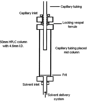
Initial work involved the development of an in-house packing method for CEC columns. The method developed, which was a pressure driven system using a Shandon HPLC packer, proved to be successful. The reliability of the retaining frit and the nature of the packing material were major factors in column performance,
Once the column fabrication process had been developed, the experimental conditions for CEC in the Prince Technology CE instrument were optimised. The results showed that in many respects the system responded as a traditional LC system would, with changes in buffer compositions, stationary phase and, in this case, EOF etc. all producing definite and reproducible changes in the separation of the test mixture. Variations in sample loading technique were investigated and a simple method developed to improve the peak efficiencies and resolution of analytes, by focussing them on the head of the column.
Contents.
Contents... 1
Glossary...4
CHAPTER 1...6
1.1 Introduction... 6
1.2. Theory...10
1.2.1. Electroosmotic Flow... 10
1.2.2. Electrophoretic Mobility...14
1.2.3. Migration Time...17
1.2.4. Selectivity...18
1.2.5. Resolution...19
1.2.6. Efficiency... 20
1.2.7. Electric Field Strength...24
1.2.8. Buffer pH... 26
1.2.9. Buffer Concentration or Ionic Strength... 27
1.2.10. Temperature... 29
1.2.11. Surface Modifiers... 31
1.3. Instrumental Overview...32
1.3.1. Injection Techniques... 33
1.3.2. Detectors... 37
1.4. Capillary Electrochromatography (CEC)...43
1.4.1. Introduction...43
1.4.2. Development of C E C ... 43
1.4.3. Theory...46
1.4.4. Applications...63
1.5. Alternative Methods... 67
1.5.1. Introduction...67
1.5.2. Open Tubular Liquid Chromatography (OT-LC)...67
1.5.3. Rigid Monoliths and Continuous Beds...69
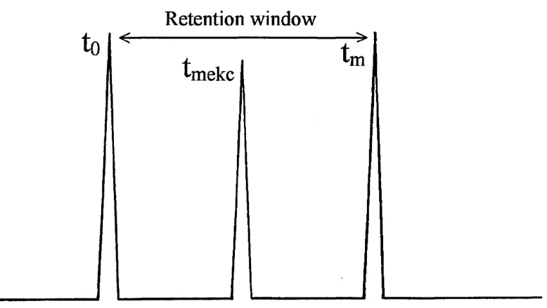
1.5.4. Micellar ElectroKinetic Capillary Chromatography (MEKC)... 71
1.6. Conclusion... 75
1.7. References...76
CHAPTER 2, Materials and Methods...83
2.1 Equipment...83
2.2 Stationary Phases...83
2.3 Reagents...84
2.4 Solutions... 84
2.5 CEC Conditions... 85
CHAPTER 3, Column Fabrication...87
3.1 Column Fabrication, Introduction... 87
3.2 Packing Procedure...87
3.3 Discussion...90
3.3.1 Column Fabrication...90
3.3.2 Retaining Frit...90
3.3.3 The Slurry... 91
3.4 Column Packing...92
3.4.1 Column Conditioning...93
3.4.2 Frit Formation...94
-3.5 Overview of Column Failures...96
3.5.1 Bubble Formation... 96
3.5.2 Localised Heating...97
3.5.3 Frit Failure... 98
3.5.4 Column Breakage...100
3.5.5 Batch to Batch Variation in Packing Material... 100
3.6 Conclusion...104
3.7 References...105
CHAPTER 4, Optimisation of Operational Parameters...106
4.1 Operational Parameters, Introduction... 106
4.2 Equipment...107
4.3 Results and Discussion...107
4.3.1 Electrolyte...107
4.3.2. Effect of pH ...112
4.3.3 Mobile Phase...114
4.3.4 Variation in Applied Voltage...118
4.3.5 Packing Material... 120
4.3.6 Column Length...124
4.4 Sample introduction... 129
4.4.1 Introduction... 129
4.4.2 Electrolyte Concentration of Sample... 129
4.4.3 Organic Content of Sample Plug...132
4.4.4 Sample Plug Length...135
4.5 Conclusion...139
4.6. Optimal Conditions... 140
4.7 References...141
CHAPTER 5, Applications of CEC... 142
5.1. Introduction... 142
5.2. Polynuclear Aromatic Hydrocarbons (PAH)...142
5.2.1. Chemicals...143
5.2.2. Procedure... 143
5.2.3. Results and Discussion...143
5.2.4. Conclusion...151
5.3. Analysis of a Test Mixture...152
5.3.1. Chemicals...152
5.3.2. Procedure... 152
5.3.3. Results and Discussion...152
5.3.4. Conclusion...156
5.4. Prostaglandins...157
5.4.1. Introduction...157
5.4.2. Available Methods for Analysis of Prostaglandins...158
5.4.3. Experimental... 159
5.4.4. Results and Discussion...159
5.4.5. Conclusion... 162
5.6. References...163
CHAPTER 6, Applications of CEC - Nicotine Metabolities...164
6.4.1. Results and Discussion... 166
6.4.2. The Effect of Electrolyte Concentration...166
6.4.3. The Effect of Buffer Additives... 168
6.4.4. Applied Voltage...170
6.4.5. Conclusion...171
6.5. Investigation utilising CEC... 174
6.5.1. Urine profile of smokers and non-smokers... 178
6.5.2. Conclusion... 188
6.6. Quantification of Cotinine in urine...189
6.6.1 Introduction...189
6.6.2 Method... 191
6.6.3 Results and Discussion... 193
6.6.4 Conclusion... 197
6.7 Reference:...199
7. Conclusion... 200
-Glossary
Pep Electrophoretic mobility
vep Electrophoretic velocity (mm s'1)
v e o f Electroosmotic velocity (cm s'1)
Pe o f Electroosmotic mobility (cm'2 V 1 s'1)
L Total length of column (cm)
I Effective capillary length, distance to detector (cm)
V Applied voltage (V)
so Permittivity of vacuum (8.85x1 O'12 C2 N'1 p'2)
sr Dielectric constant of the mobile phase
% Zeta potential (mV)
t| Viscosity of the mobile phase ((water) 0.089 g cm'1 s'1 at 20°C)
E Electric field strength (V cm'1)
ct Charge density at the surface of the shear
R Gas constant (8.315 J K'1 mol'1)
T Temperature (K)
F Faraday constant (9.65x10⁴ C mol'1)
q Charge of particle
r Stoke’s radius of particle (pm)
c Electrolyte concentration (mol L'1)
8 Thickness of the double layer (nm)
e Charge per unit surface area
A Molar conductance (Q"1 m2 mol'1)
R Resistance (Q or V A'1)
I Current (A)
W Watts (J s'1)
-CHAPTER 1
1.1 Introduction.
Electrophoretic separations have been demonstrated for over a century (1).
However, it was not until the work of Tiselius (2) in the 1930s, for which he
obtained the 1948 Nobel Prize, that interest in electrophoretic separation
began to gain momentum. Tiselius had developed moving boundary
electrophoresis in free solution, thus allowing the separation of proteins in
complex biomedical samples that by normal methods would be unresolvable.
One of the problems observed in electrophoretic separations was that of
diffusion arising from convection in the bulk solution due to Joule heat, which
reduced the efficiency of the separation. Therefore, support media were
developed to reduce convection in the columns. Materials employed included
cellulose powder, grains of starch or plastic, glass wool and various gels such
as silica, agar, agarose, starch and polyacrylamide (3). Some of these are still
routinely used today in many biomedical laboratories, in the form of slab gel
electrophoresis, with the most commonly used support being that of a
polyacrylamide gel. However, there are problems associated with the use of
these support phases, principally that of adsorptive and steric interference
which hinder reproducibility and sensitivity.
Another method that was developed to reduce unwanted convection
In 1974 Virtenen (6) described the potential advantages of using capillary
columns instead of the larger bore columns that had been used up to that
date. This theory was later proven by Mikkers et al. in 1979 (7), who described
electrophoresis in a 200 pm ID PTFE capillary. The initial results were poor as
the sample was overloaded to overcome the poor detector sensitivity.
Jorgenson and Lukacs, in 1981 (8,9), were the first to demonstrate the true
potential of Capillary Electrophoresis (CE). They used fused silica capillaries
similar to those employed in GC, showing that high efficiencies could be
obtained using columns with an internal diameter of less than 100pm.
Throughout the 1980s the development of CE was limited. However, towards
the end of this decade interest in CE increased, which in part may be
explained by the introduction of commercially available instruments. The
availability of such instruments allowed CE to become more accessible to a
wider range of groups. Prior to this CE had been developed on home-made
instruments.
Since the initial demonstration of free solution electrophoresis as a viable
analytical technique by Jorgenson and Lukacs, various methods have been
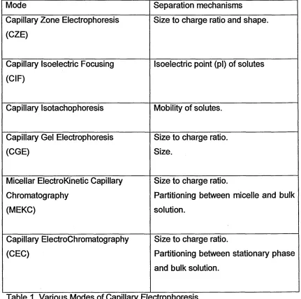
developed to allow a greater range of solutes to be separated (Table 1). Many
of the principles had been developed in the 1950s and 60s with the
Mode Separation mechanisms Capillary Zone Electrophoresis
(CZE)
Size to charge ratio and shape.
Capillary Isoelectric Focusing (CIF)
Isoelectric point (pi) of solutes
Capillary Isotachophoresis Mobility of solutes.
Capillary Gel Electrophoresis (CGE)
Size to charge ratio. Size.
Micellar ElectroKinetic Capillary Chromatography
(MEKC)
Size to charge ratio.
Partitioning between micelle and bulk solution.
Capillary ElectroChromatography (CEC)
Size to charge ratio.
[image:15.616.66.497.28.456.2]Partitioning between stationary phase and bulk solution.
Table 1. Various Modes of Capillary Electrophoresis.
The majority of the separations result from differences in the size to charge
ratio of the solutes, and hence differences in electrophoretic mobility, allowing
them to be separated into discrete bands. The one potential disadvantage is
that neutral species have no electrophoretic mobility and are consequently
drawn through the column with the bulk flow without any separation. This
developed and these will be discussed briefly to give an overview of possible
1.2. Theory
1.2.1. Electroosmotic Flow.
The Electroosmotic Flow (EOF) leads to the bulk movement of solution
through the capillary and is generated by a surface charge on the capillary
wall. This is produced by ionisation at the inner wall of the capillary and/or the
adsorption of ions onto the inner surface (10).
Capillary columns used in CE are made from fused silica and the inner
surface is covered by silanol groups ( -Si-OH). The pKg of the silanol group is
approximately 2.2 and dissociation occurs to give silanoate groups ( -Si-O').
Above pH 7-8, the silanol groups are totally dissociated.
When an electrolyte solution is introduced into the capillary, the surface
becomes coated by counter ions, i.e. cations, to form two distinct layers at the
capillary wall (Figure 1). The first layer is bound tightly to the surface and is
referred to as the Stern or fixed layer. The second layer is formed due to the
fixed layer being unable to completely neutralise the wall’s charge. In this
region the cations are more diffuse and can move between this layer and the
bulk solution. This region is the Gouy-Chapman or mobile layer. At the
interface of the two regions there is an electrical imbalance between the
Capillary surface
Stem layer
Plane of Shear______ + + + + +
+ + + + + + + + +
+ + +
+ + +
Gouy-Chapman Layer + + +
+
Bulk solution ,
+ EOF + + +
Figure 1. Electrical double layer at the surface of a capillary wall.
The magnitude of the flow is in part dependent on the electophoretic mobility
of the electrolyte and also the formation of the double layer at the capillary
surface, which can exert an additional force on the observed electroosmotic
flow.
This is the result of the cations in the mobile layer being attracted towards the
cathode. The movement of this layer causes bulk solution migration towards
the cathode, as the ions in the diffuse region draw the ions in the bulk solution
along, creating the electroosmotic flow.
The magnitude of the EOF is controlled by the zeta potential. The zeta
potential is described as the potential difference between the fixed and mobile
Where, 5 is the double layer thickness, e is the charge per unit area and sr is
the dielectric constant.
The zeta potential is dependent on pH and electrolyte. A higher pH value will
mean a greater number of silanoate groups (surface charge) to be present, so
increasing pH increases the zeta potential and hence the EOF increases.
However changing the electrolyte has only a small effect on the EOF, if all
other parameters remain the same.
The thickness of the double layer (8) is proportional to the zeta potential.
Therefore the size of the double layer can also affect the EOF. The double
layer has a finite thickness, which falls away exponentially. (Figure 2).
STERN LA Y E R
IP L A N E OF
' c u p a CHARGE
DENSITY (o)
GOUY-CHAPM AN LAYER
The thickness of the double layer can be calculated by using the equation:
5 = SQSrR T 2cF
0.5
eq. 1.02
Where, s0 is the permittivity of a vacuum, er is the dielectric constant, R is the
gas constant, T is the temperature, c is the concentration of the electrolyte
and F is the Faraday constant.
Therefore the concentration of the buffer also plays a part in determining the
magnitude of the EOF, as well as the pH and type of electrolyte used. As the
concentration of the electrolyte is reduced the double layer thickness is
increased, thereby increasing the Zeta potential and hence the velocity of the
EOF. This increase in EOF is actually dependent on the ionic strength of the
electrolyte, so factors other than concentration (e.g. ionic charge and radius)
are also important, which the dielectric constant of the electrolyte indicates.
In general, the thickness of the double layer is inversely proportional to the
electrolyte concentration e.g. a buffer containing 10mM of electrolyte will give
rise to a double layer of approximately 1nm thickness (11). The narrowness of
the double layer formed means that, as an approximation, the EOF can be
1.2.2. Electrophoretic Mobility.
When a charged species is placed under the influence of an electric field, it
will migrate towards the electrode of the opposite charge at a given rate i.e. its
electrophoretic velocity (vep). The rate at which the solute travels through the
solution is dependent on its charge and size and is known as its
electrophoretic mobility. The electrophoretic mobility of an ion (pe) can be
defined as
v . ~ - r -4 nrp- e(i- 1 0 3
where, q is the charge on the ion, r| is the viscosity of the bulk solution and r is
the radius of the ion.
Anions
Neutrals
Cations
©
Anode
Figure 3. Various migration rates observed in CE.
Figure 3 shows that in CE the mobility of the solute particle is not only
determined by its charge, but its size as well. This means that a small particle
has a greater electrophoretic mobility than a larger particle of similar charge.
discrete band at the same rate as the running buffer (as q is equal to zero,
hence their electrophoretic mobility is zero).
The electrophoretic velocity of an ion is proportional to the electric field placed
across the system. The electrophoretic velocity (vep) can be defined as
vep = M*E eq. 1.04
where, E is the electric field strength (E=voltage/length).
When placed in the buffer, individual ions are surrounded by counter ions,
which form a double layer around them. Therefore the particles have
individual zeta potentials, which are related to their electrophoretic mobilities.
This relationship can be seen in the Helmholtz and Smoluchowski equation:
eq-'i'° 5
where, peff is the effective electrophoretic mobility of the ion, s is the dielectric
constant and ^ is the effective Zeta potential.
It should be noted that the electroosmotic mobility of the bulk solution can be
calculated using equation 1.05.
Equations 1.03 and 1.05 also show that the viscosity of the buffer affects the
movement of the analyte in solution. The viscosity affects the movement by
15-increasing or decreasing frictional drag, depending on the relative viscosity of
the solvent being used.
This means therefore that electrophoretic velocity is dependent on the mobility
of the particle in the electrolyte used and the size of the electric field that is
applied across the capillary. The observed velocity of a particle is thus
dependent on two factors, its electrophoretic velocity and the velocity of the
EOF, as shown in equation 1.06.
K b s = K + v e o f e q . 1 0 6
This explains why simultaneous separations of cations and anions are
possible. In the normal mode of operation, solutes are loaded at the anode
and are detected at the cathode. The velocity of an ion through the column is
dependent on its charge and size (Figure 3). Neutral compounds migrate at
the same rate as the EOF, as they have no effective charge and are neither
attracted nor repulsed by either electrode. The migration rates of cationic and
anionic species vary according to their respective charge and size, therefore
allowing separations to be achieved by differences in electrophoretic
velocities. The velocities of cations are enhanced by the EOF, whilst anions
can be drawn through the capillary if the velocity of the EOF is greater than
1.2.3. Migration Time.
The linear velocity of the EOF through the capillary can be measured by use
of a neutral marker added to the sample solution. Examples of such markers
include thiourea, acetone and mesityl oxide. Migration times (tm) may be
calculated using equation 1.07.
Where, i is the effective capillary length i.e. distance to the detector.
The migration time of a neutral marker will allow the determination of vobs for
the EOF. The electrophoretic velocity of a charged solute can also be
determined from this equation by substituting in the migration time.
Additionally the observed electrophoretic velocity of an ion can be calculated
by equation 1.08
Substituting equation 1.07 into equation 1.08, when E is equal to V/L will give
therefore, vobs= — eq. 1.07
m
V obs ~ (M e + MeOf\ E eq. 1.08
M e MeOF y _ J _
V L y tm eq. 1.09
Where, V is the applied voltage and L is the total capillary length.
Rearrangement of eq. 1.09 leads to eqs. 1.10 & 1.11, from which
( I L \ eq. 1.10
M e ~ y MeOF
k. " m ' a
V m
IL eq. 1.11
(Me + MeOfW
Equation 1.10 indicates that short columns, coupled with a high applied
voltage, will give rise to reduced migration times.
1.2.4. Selectivity.
The selectivity of a separation can be defined as the degree of separation that
is achieved between two consecutive solutes upon detection. Selectivity (a),
is calculated using equation 1.12. When there is no selectivity a= 1, and as
selectivity increases, a increases.
a = —— — eq. 1.12
h ~ ^nm
Where, ti and t2 are the migration times of the solutes and tnm is the migration
time of a neutral marker.
Selectivity can also be considered as a function of the ratio of the effective
electrophoretic velocities of solutes. Electrophoretic velocity, vep, can be
calculated using eq. 1.13, which in turn can be used in eq. 1.14 to determine
selectivity. It is also possible to derive selectivity from the effective mobility of
eq. 1.13
a = — .Const. eq. 1.14
a - — .Const. eq. 1.15
1.2.5. Resolution.
Resolution (R) can be defined as the degree of separation that is achieved
between two peaks and can be calculated by equation 1.16, which is
dependent on the migration times (t) and peak widths (w) of the two solutes.
where At is the difference in migration times of the solutes (where ti and t2 are
the migration times of the solutes), and wave is the average peak width (where
Wi and W2 are the peak widths of the solutes).
The peak widths, and hence peak efficiencies, of the solutes have a direct
effect on the resolution, as do their electrophoretic mobility. Hence equation
1.17 can be used to determine resolution.
A/ eq. 1.16
W,1 1 rr2 + wave
-19-R = l/41
/
eq. 1.17Where, Apapp is the difference in the mobilities of the solutes, pave is the
average mobility of the solutes and N is the peak efficiency (see equations
1.18 and 1.19).
1.2.6. Efficiency.
In chromatography, efficiency is a measure of the number of theoretical plates
produced by a column, where the greater the number of plates the more
efficient is the separation. The increase in efficiency comes from a greater
number of interactions of the solutes between the two phases. However,
efficiency is reduced due to dispersive effects in the column, resulting in band
broadening. Efficiency (N) can be calculated using either peak width at half
height (W1/2), or base width (Wb), shown in equations 1.18 and 1.19
respectively.
f \2
N = 5.54 —
w„ eq. 1.18
Where, W1/2 is peak width at half height.
eq. 1.19
Where, Wb is peak width at base.
This allows the effect of individual factors to be assessed. HETP can be
calculated using several equations, for example eqs. 1.20 and 1.21.
HETP = — = — eq. 1.20
N L
Where, L is the total capillary length and is the total variances or the sum
of all the dispersive effects in the system.
The alternative method would be to use the Van Deemter equation for plate
height (eq. 1.21)
HETP = A + b/ + Cv eq. 1.21
Where, A, B and C are constants and v is the flow velocity.
Each of the constants in equation 1.21 relates to one of the dispersive
mechanisms and how it is affected by the flow velocity. Therefore the flow
needs to be optimised to minimise the dispersive effects, which lead to a
reduction in HETP.
The A term or eddy diffusion, takes into account the numerous different paths
that a solute can travel as it passes through a column. It is independent of the
velocity of the flow. B/v or longitudinal or axial diffusion occurs as the solute
diffuses into the surrounding solution, thereby increasing the width of the
sample zone. This effect is greater the longer the solute is on the column,
therefore use of a high velocity can minimise it. Cv relates to the rate of
-21-equilibration of the solute between the two phases. To reduce broadening due
to this effect the flow velocity needs to be minimised.
CE is not a true chromatographic technique, as the analytes are separated by
differences in their electrophoretic mobilities, instead of differing partition co
efficients, as in HPLC. Therefore, in CE efficiency is mainly a measure of peak
shape and width. However, the electroosmotic flow generated in an open
capillary column does have one major dispersive mechanism, that of
longitudinal or axial diffusion (B/v term). Eddy diffusion and rate of
equilibration do not apply to CE, hence the terms A and Cv are eliminated.
In addition to the reduction in dispersive mechanisms, bulk solution movement
through the capillary has a flat or plug profile. This is in contrast to a pressure
driven system that has a parabolic flow profile. Therefore, an increase in peak
efficiency can be observed in CEC due to the nature of the bulk flow (Figure
4).
The degree of axial diffusion over a given time can be determined using
spatial variances (a 2). Assuming that there are no other dispersive effects
acting on the solute, equation 1.22 applies.
a 2 = 2Dt eq. 1.22
* *
b.
A
Figure 4. Flow profile in a column with (a) electro-drive and (b) pressure drive.
There are however several other dispersive forces acting on the zone as it
migrates through the column, which can affect the total amount of axial
diffusion that is observed. The total variance is the sum of several other
variances that are found in the system (equation 1.23).
Where, <r£is the variance due to molecular diffusion, <r^is variance arising
from sample injection, c^et is variance due to the detector and a] is variance
due to other dispersive effects including solute adsorption, Joule heating,
electromigration dispersion and nonuniform flow profile. These effects will be
discussed in later sections.
=CT2D+ a lj+ (7 2det+Or20 eq. 1.23
-23-1.2.7. Electric Field Strength.
As previously discussed, the electrophoretic velocity of a solute and the
magnitude of the EOF are in part derived from the electric field strength (E)
that is placed across a capillary column. The strength of the electric field is
dependent on two factors, the applied voltage (V) and column length (L),
(equation 1.24)
To decrease the analysis time the electric field needs to be maximised. The
voltage is regulated in most commercial CE instruments to between ±30Kv.
Variations in the capillary column length can be used to vary the strength of
the electrical field. However, increasing the electric field strength can result in
increased Joule heating.
In a CE instrument, conductivity can be related to the conductive medium (the
electrolyte) and the dimensions of the capillary. This may be expressed by
equation 1.25.
RA
kl.
„
K = --- or R = — eq. 1.25
L A
Where, R is resistance, A is cross sectional area of column and K is
When an electric potential is placed across a capillary column containing a
solution of electrolyte a current is produced. Most of the energy that enters the
system is converted into heat. The quantity of heat that is generated is
proportional to the amount of power that is applied to the system. The heat
that is generated is referred to as Joule heat. The rate of heat generation (P)
is expressed in equation 1.26.
P = VI eq. 1.26
Where, I is the current and V is the applied voltage.
Or in terms of V and R by substituting Ohm’s law (F = IR) into equation 1.26,
to give equation 1.27.
V2
P = — eq. 1.27
R
This is then substituted into equation 1.25, to give the rate of heat generated
in an enclosed system (see equation 1.28), given that K = AC and A = nd2/ 4
p = ^V ^ _ eq. 1.28
4ACL
Where A is the molar conductivity of the solution, C is the concentration and d
is the diameter of the column.
Equation 1.28 indicates therefore that the rate of Joule heating is dependent
on the type and concentration of the buffer and the column diameter. As the
-25-internal diameter of the column is reduced, so the current produced is also
decreased. Therefore, if the internal diameter is halved then the current will
decrease four fold (or the square of change in the I.D).
1.2.8. Buffer pH.
The pH of the buffer plays a vital role in CE, as it not only determines the
magnitude of the EOF that is developed but also the effective mobility of the
analytes.
As previously discussed, the EOF is derived in part from the surface charge,
therefore as the pH rises so does the EOF. Variations in surface charge affect
the zeta potential, which is one of the factors that affect the generation of the
EOF and electrophoretic mobility of the solute. When an ion is placed in
solution a double layer is formed around it. This double layer acts in a similar
manner to that found at the surface of the capillary. Therefore changes in
composition of the running buffer can affect the electrophoretic mobility of the
ion, according to the Helmholz and Smoluchowski equation (see equation
1.05).
The electrophoretic mobility of an ion may also be varied with pH by altering
its effective charge. The degree of dissociation (oc) of a solute is related to its
pKa, therefore the effective mobility of the solute varies according to equation
1.29.
The pH is chosen to allow the optimal separation of the analytes, while not
necessarily trying to optimise the velocity of the EOF. This is particularly
useful when analytes have the same or similar pKa values, allowing the
selection of a pH that will increase the electrophoretic mobility of one over the
other.
1.2.9. Buffer Concentration or Ionic Strength.
As the concentration or the ionic strength of the electrolyte is decreased, the
resultant EOF is increased. A high EOF is not always required, as good
resolution is generally preferred over rapid analysis times. This requires a
higher concentration of buffer or an increase in the ionic strength of the
electrolyte to lower the zeta potential and hence to slow the EOF (13).
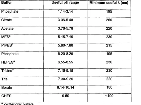
Generally, an inorganic buffer has a higher ionic strength than an organic
buffer of the same concentration. Therefore, when choosing a buffer, it is
important to take into account both its conductive properties and its effective
pH range (see Table 2).
If short analysis times are required low electrolyte concentrations can be
used. However, problems can arise if the concentration used is excessively
low, resulting in band broadening and asymmetric peaks. This is due to
differences between the conductivity of the buffer and the sample plug, which
can cause distortions in the electric field.
When the ionic strength of the buffer is significantly in excess of the sample
plug’s, a reduction in the peak distortions and an increase in sensitivity can be
-27-observed. If a sample is dissolved in running buffer it can produce a significant
lowering in the limit of detection, compared to that of the same sample being
dissolved in either 10% buffer solution or in 100% water. This is due to the
sample plug having a slightly different conductivity to that of the bulk solution,
causing a stacking effect at the interface of the two zones. At the interface the
electrophoretic velocity of the solute is decreased, due to the higher
concentration of electrolyte in the bulk solution, which reduces the solute’s
Zeta potential thereby focussing the solute before it migrates into the bulk
solution. Without this interface the solute will diffuse into the bulk solution,
leading to band broadening and peak tailing or fronting, depending on the
Buffer Useful pH range Minimum useful X (nm)
Phosphate 1.14-3.14 195
Citrate 3.06-5.40 260
Acetate 3.76-5.76 220
MESa 5.15-7.15 230
PIPES3 5.80-7.80 215
Phosphate 6.20-8.20 195
HEPES3 6.55-8.55 230
Tricine3 7.15-9.15 230
Tris 7.30-9.30 220
Borate 8.14-10.14 180
CHES 9.50 <190
a Zwitterionic buffers.
Table 2. Commonly used buffers in capillary electrophoresis and their associated properties. (12).
1.2.10. Temperature.
Temperature control is important in CE as elevated temperatures can cause
various problems. Increases in temperature are the result of joule heating;
even a one degree rise increases the electrophoretic mobility of an ion by 2%
(14). As the temperature rises so does the conductivity. This is due to the
decreasing viscosity of the buffer, which leads to increased current. A thermal
gradient is produced through the column, creating convection currents, which
leads to a parabolic flow profile. The magnitude of these distortions is related
to the quantity of heat that is produced and the rate at which it dissipates. This
can be affected by the column’s internal diameter, the thickness of the column
[image:36.616.60.532.26.376.2]-wall and the thermal properties of the column material. However, the upper
limit for the column’s I.D has been reported by Knox (15) as being about
200pm, as above this value the column cannot effectively dissipate the heat
that is generated at its centre.
Elevated temperatures may also lead to band broadening and irreproducible
migration times, due to convection currents and temperature gradients in the
capillary altering the EOF that is being generated. Denaturation or
decomposition of samples, especially those of biological origin, may also
result from increases in temperature.
In extreme cases, for example if the buffer temperature rises, the CE
instrument can automatically shut itself down, as the current generated would
exceed the maximum operational limits of the instrument and if left would
eventually lead to the buffer boiling.
However, when temperature is used in a controlled manner to aid separation
there can be several potential advantages to be gained. The most apparent is
the decrease in migration time due to the reduction in viscosity, which results
in a greater EOF.
Variations in temperature can also enhance the resolution that can be
dramatic reduction in analysis time. This was only possible as a result of a
structural reconfiguration of the proteins at elevated temperatures, which
aided their movement through the gel.
It must be noted that with a change in the temperature there is also an effect
on the volume of the sample loaded onto the capillary, which must also be
taken into account. This is due to the changes in the density of the liquids with
variations in temperatures.
1.2.11. Surface Modifiers.
Flow modifiers are used to alter the magnitude and the direction of the EOF.
There are three potential effects that a modifier can have on the EOF. It can
either reduce, eliminate, or reverse the EOF. This is achieved by blocking or
altering the charge on the capillary wall. The use of modifiers can, therefore,
be used to improve resolution by reducing the magnitude of the EOF or
decrease the analysis time for anions by reversing the flow. An untreated
fused silica column can act as a cation exchanger, due to the weakly acidic
silanol groups present on the surface of the capillary. Therefore, the capillary
surface needs to be modified to reduce any interactions between the cationic
solutes and the capillary surface as these interactions lead to a loss of
efficiency and irreproducible migration times. Capillaries can be coated in one
of two ways, either by dynamically coating the surface with surfactants or by
permanently altering the surface by covalently bonding different groups to it.
-1.3. Instrumental Overview.
All capillary electrophoresis (CE) instruments are similar to each other in their
basic design. A schematic is shown in figure 5. The basic configuration
employs two electrolyte reservoirs bridged by a length of fused silica capillary,
which can have an internal diameter of 10pm - 200pm. Electrodes are placed
in the electrolyte reservoirs and are connected to a high voltage power supply
capable of providing up to 30Kv. A current limit of between 200pA and 300pA
is usually found on most instruments. An electrical circuit can be established
once the capillary is filled with the electrolyte. The application of a voltage
across the capillary results in the production of an electroosmotic flow through
the capillary.
Temperature controlled compartment
Capillary
Detecror
Anode Cathode
Integrator
{ Power Supply }
[image:39.615.114.435.376.608.2]Many of the detectors that are being employed are also used in modern
HPLC. The graphical representation of the data that is collected is referred to
as an electropherogram instead of a chromatogram as in HPLC separations.
1.3.1. Injection Techniques.
The small sample volume requirements of the CE necessitate special injection
methods and several different techniques have been reported that will deliver
sample into the capillary. These include an electric sample splitter (17),
rotary-type injector (18), freeze plug injections (19) and microinjection (20). However,
commercially available instruments load samples by either electrokinetic or
hydrodynamic methods.
1.3.1.1. Hydrodynamic Injection
1.3.1.1.1. Pressurisation.
The sample is introduced by the application of pressure to the sample vial,
which forces the sample into the capillary. The volume of solution injected on
column (V|) is calculated by the Poiseulle equation, (equation 1.30).
APrjz^ eq. 1.30
8 rjL
Where, AP is the pressure drop across the capillary, r is the internal radius of
the capillary, L is the total length of the capillary and tj is the injection time.
The plug length (Lp) can then be calculated as follows
vi APr2/;. , _
L = ~ = L eq. 1.31
nr %r\L
Variations in the volume of sample loaded will affect peak area and height.
This can occur due to siphoning if the ends of the capillary are not level with
-each other. Changes in temperature can also affect the volume loaded by
altering the hydrodynamic properties of the solutions.
1.3.1.1.2. Gravity Loading.
Samples introduced by gravity flow are siphoned into the capillary by lifting the
sample vial above the outlet vial. The sample volume introduced can be
calculated from
p G a /A fa , 32
'
%t]L
Where, p is the density of the buffer, G is the gravitational constant and Ah is
the difference in the heights of the liquids.
1.3.1.2. Electrokinetic Loading.
Electrokinetic loading can be used in CZE and when there is insufficient
pressure available to load the sample, such as in gel electrophoresis or
capillary electrochromatography. The sample is loaded by a combination of
EOF and the electrophoretic mobility of the sample ions. The quantity of
solute loaded (Qjnj) can be calculated by,
+/ v V 2^'.
L
= f: — ~-C eq. 1.33
Where C is the concentration of solute, p is the electrophoretic mobility of the
solute and pe0f is the electrophoretic mobility of the running buffer.
peak area and height will increase proportionally with increasing
electrophoretic mobility. Heung et al. (21) showed that sample bias could be
corrected by the use of a bias factor b, as seen in equation 1.34. This ratio
can then be used to correct the peak area or height of the solutes.
where, m andp2 are the electrophoretic mobilities of the solutes and ti and t2
are the migration times of the solutes.
Differences in the ionic strength or the pH between the buffer and sample can
affect the quantity of ions loaded and the efficiency of the separation. These
effects can be minimised by dissolving the sample in the buffer, or by the
addition of a non-detected ion to equalise the relative conductivities of the
sample and buffer.
A side effect of the sample bias is that of sample depletion, especially with
replicate injections from the same source. With multiple injections the
concentration of the more mobile solutes will decrease disproportionally to
that of the less mobile solutes. This results in variations in the amounts of
solutes loaded and a decrease in ionic strength of the sample. eq. 1.34
-35-1.3.1.3. Sample Overload.
With the low sample volumes used in CE it is easy to overload the capillary
column. By overloading the capillary, the maximum number of theoretical
plates (Nmax) that can be obtained is reduced, leading to a less efficient
separation (see equation 1.35).
JV = 12max
r
\ 2
eq. 1.35
\< lm j J
Where q;nj is the volume of the sample injected and qc is the volume of the
column.
Aebersold and Morrision (22) suggest that as a rule of thumb, the injection
plug should be 1 to 5% of the total volume of the capillary.
Another potential problem relates to differences in conductivity between the
sample plug and the bulk solution. This can lead to an electric field variation
along the capillary, which can result in either distorted peaks or focussing of
the solutes.
1.3.1.4. Extraneous Injection.
Variations in the quantity of sample loaded may occur as a result of several
different processes!
• Movement between the buffer and the sample solutions due to convection
as a result of differing thermophysical properties of the solutions, such as
viscosity, surface tension and density.
• The longitudinal diffusion of the solutes in the buffer solution, due to
differences in the relative mobilities of the solutes and the electrolyte in the
buffer.
1.3.2. Detectors.
CE has been coupled to a wide variety of detectors, many of which are
already well established in HPLC. These detection methods include
fluorescence (23-26), laser induced fluorescence (27,28), amperometry
(29,30), conductivity (31,32), refractive index (33,34), laser Raman (35,36),
radiometry (37,38), NMR (39,40) and MS (41). The most common detector is
the UV/Vis absorbance detector, which has been utilised in this study. Table 3
lists approximate detection limits for some of the detectors used in CE (42).
Detector Approximate Detection Limits
Moles Molarity3
UV/Vis absorbance 10‘l3-1(r10 10‘6-10‘'
Indirect absorbance KT^-IO-10 K T -IO *
Fluorescence 1 0 '-1 0 a
Indirect Fluorescence 10'14-10'16 10^-10‘8
Laser-induced Fluorescence iO'18- i ( r !U 10‘13-10'1b
Mass Spectrometry 10'lb-10'1' 1 ()-*>-10'1 u
Amperometric 10 18-10"la 10''-10'1U
Conductivity 10-lb-10-lB 10‘'-10‘u
Refractive index lO-’O-io-'t; lO’h-IO'8
Radiometric 10'lu-10'lid
a Depends upon volume of sample injected.
Table 3. Detectors which have been coupled to CE with their approximate detection limits (42).
-37-1.3.2.1. UV/Vis detector.
The UV detector utilises changes in the quantity of light that is passed through
a detection window or cell as a solute migrates past the detection window.
The transmittance of light through the column is given by equation 1.37.
T = — eg. 1.37
L
Where, I0 is the light intensity of the initial beam of light and I is the transmitted
light intensity after passage through the capillary.
As a solute passes through the beam of light at the detection window, the
solute will absorb a certain quantity of this light. Beer’s Law, equation 1.38,
defines the absorbance (A) of the solute.
A = log— = d>c eq. 1.38
T
Where, s is the molar absorptivity, b is the path length and c is the
concentration of the solute.
The detection wavelength chosen has to maximise the absorbance of the
chromophores present in the solute, while minimising the background
absorbance i.e. direct UV detection. However, if the solutes do not absorb
light the buffer needs to have a high absorbance, with the wavelength set to
allow the maximum difference in absorbance between the solutes and the
The detection cell path length is also an important factor to be considered, as
the path length is directly proportional to the absorbance observed. To
maximise the absorbance and hence sensitivity, the path length needs to be
as large as possible (this will be discussed in section 1.3.2.2).
There are two types of UV detectors, single variable wavelength
(monochromatic) detectors and multiple wavelength photodiode array
detectors, with the latter being able to observe the entire spectrum
simultaneously.
1.3.2.2. Detection Window.
In CE, detection is usually achieved on column. Therefore, the polyimide
coating supporting the fused silica needs to be removed to produce a suitable
detection window. There are several means of removing the polyimide. The
first is to burn the polyimide off by using either a Bunsen flame or an
electrically heated filament. The use of a Bunsen flame may be convenient but
it produces a large and unstable detection window that is easily broken. The
heated filament allows a great deal of control in the size of the detection
window formed (1-3mm), allowing a more stable window to be produced,
however, heating the fused silica can damage it. The second method would
be to dissolve the polyimide by use of boiling concentrated sulphuric or nitric
acid, which does not damage the fused silica and is useful when the inner
surface of the capillary has been modified. The final method is to remove the
polyimide with a sharp knife, however the silica column can be easily
scratched, causing optical distortions and weak points.
-39-The detection cell is part of the capillary. This means that the path-length is
equivalent to the internal diameter of the capillary being used. A large internal
diameter will give greater sensitivity, however, with larger internal diameter
columns Joule heating can occur, as the current generated is proportional to
the square of the internal diameter. A result of this several novel detection
cells have been developed, which allow greater sensitivity to be achieved.
The Z-cell (43,44) works by forming a small section of capillary that is
perpendicular to the rest of the column, as shown in figure 6, which is then
used as the detection cell. A 3mm path length in the Z-cell will increase
sensitivity by ten-fold (45) over that of a straight capillary.
Detector cell
Light source Detector
Figure 6. Diagram of a Z-cell.
The use of a rectangular column was reported by Tsuda et al. (46). The
capillary was formed to give a path length of 1000pm along one axis. The
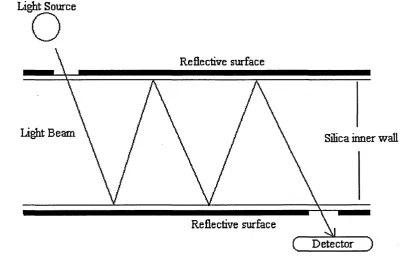
The multireflection cell (47,48) works by removal of the polyimide to allow the
surface to be coated with silver backed by an outer coating of black paint.
The silver is used like a mirror to reflect light along a given path length inside
the column, as shown in figure 7. The increase in sensitivity is not quite
proportional of the increase in the cell path length, which is due to a small
reduction in the intensity of light with each reflection.
Light Source
The bubble cell is produced by either blowing or etching a bubble into a
section of the capillary producing an increase in sensitivity proportional to the
increase in the column internal diameter. This has been shown to provide a
threefold increase in sensitivity when a 50pm column had a 150pm bubble cell
fabricated within it (49).
Reflective surface
C Detector )
Silica inner wall
Figure 7. Diagram of a Multireflection cell.
[image:48.613.66.475.214.477.2]-The sleeve cell (50,51) works by carrying out the separation in a normal
capillary column i.e. 50pm, which is then butted up against a wider bore
column e.g. 200pm, to be used as the detection cell, (see figure 8). As the
buffer flows into the cell, the flow is reduced to compensate for the increase in
volume, thereby compressing the peak bandwidth. The compression of the
bandwidth allows for sharper peaks and hence an increase in sensitivity in
addition to the gain from the longer cell path-length.
Capillary
Sleeve
light Source
Detector
[image:49.614.111.408.250.545.2]1.4. Capillary Electrochromatography (CEC).
1.4.1. Introduction.
As the theory of CE would indicate, ions can be readily separated on the basis
of their charge and size. However, if the compounds of interest are neutral,
they cannot be separated under the same conditions, as all uncharged
solutes irrespective of size migrate through the capillary at the same rate as
the bulk solution. Several methods have been developed to address this
problem.
In this study capillary electrochromatography (CEC) was investigated and
developed as a possible routine method for separation of neutral compounds.
The background to CEC will be discussed in the following section, along with
a summary of the other electrophoretic techniques that could be utilised.
1.4.2. Development of CEC
The development of CEC can be traced back to Strain in 1939 and Lecoq in
1944, who were the first to report the generation of an EOF in liquid
chromatography (52). Prior to the work of Pretorious et a/. (53) in the mid 70s
and Jorgenson and Lukacs (9) in the early 80s, the electrically driven bulk
movement of an eluent through a porous material had been discussed, but
never demonstrated as a viable analytical technique.
In 1974, Pretorius et al. (53) reported the effect of using an applied voltage
instead of pressure to move an unretained compound through a packed
electrochromatography (EC) experiments were performed. The results
supported the theory that band broadening commonly found in HPLC would
be reduced, due to the flat flow profile generated by the EOF in EC.
In 1981 Jorgenson and Lukacs (9) reported data obtained on a crude
non-aqueous CEC system using a 170pm I.D. column. Unlike the work of
Pretorius, the compounds were partially retained on the column in their
investigation. This work, as they freely admitted in the paper, was a crude
attempt at CEC but did indicate that highly efficient separations were possible.
In 1983, Stevens and Cortes (13) cast doubt on the viability of CEC. Their
investigation looked at various sizes of packing material. They concluded that
if the packing material was smaller then 50pm in diameter there would be
insufficient flow generated to allow effective separations to take place. Double
layer overlap degrading the EOF was suggested as a possible explanation for
their observations.
The conclusions of Cortes and Stevens were dismissed by Knox and Grant in
1987 (54), in their theoretical paper on miniaturisation of chromatography
systems. This included a purely theoretical study of CEC. They determined
the potential double layer thickness around particles in the stationary phase
and then compared it to the mean channel size in the packed bed. They
predicted the maximum electrolyte concentration (10mM) and the minimum
Knox and Grant later confirmed their hypothesis in 1991 (55). It was at this
time that renewed interest in CEC began.
The initial development of CEC led to a variety of terms being employed to
described this technique. These included titles such as liquid chromatography
with electroosmotic flow (56), electro-endosmotically driven liquid
chromatography (54), electrically driven liquid chromatography (57),
electroendosmotic capillary chromatography (58) and electrokinetic
chromatography with packed capillaries (59). Tsuda (60) was the first to use
the term capillary electrochromatography. However, Knox, in 1994 (61)
proposed that CEC should be adopted as the official title and this term has
become accepted.
The development of CEC following the work of Knox has been slow but
steady. Several recent reviews have been published on the state of CEC.
General reviews on the fundamentals of CEC have been published by Cikalo
et al. (62), Colon et al. (63, 64), Crego et al. (65), Kowalczyk (66), Steiner et
al. (67) and Angus et al. (68). Dittmann et al. (69) reviewed the theory of CEC,
while Rathore and Horvath (70) compared the differences in LC, CE and CEC.
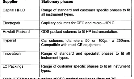
Pursch and Sanders (71) reviewed the development of stationary phases. The
steady development of CEC is reflected in the publications of Altria et al. (72)
and Euerby et al. (73), which both review the current applications available for
CEC and Krull et al. (74), which reviews progress in specific biological
applications.
-45-1.4.3. Theory.
1.4.3.1. Electroosmotic Flow in CEC.
As discussed in section 1.2.1 the EOF is generated near to the inner surface
of the capillary. The same basic principle applies to CEC columns. Stationary
phases in general are supported on silica particles, thus allowing a double
layer to be formed around each particle, similar to that at the surface of the
capillary (Figure 9). Once an electric field is applied, the cations in the diffuse
layer around the packing materials and capillary wall are drawn towards the
cathode, causing flow of the bulk solution thorough the packed column.
+
Capillary
wall
Surface of
Shear
4 ^
! ^Stationaiy phase
particles
EOF
Figure. 9. Diagram showing how an electroosmotic flow is generated on a packed column.
To allow the generation of an EOF through a packed column, the channel size
between the packed particles needs to be greater than twenty times the
thickness of the double layer that is formed around each particle (75). When
the channel size falls below this value double layer overlap can occur, which
It must be noted that the observed velocity of the EOF is the averaged velocity
of the flow rates in both the packed and unpacked sections of the capillary
(76); the flow through the packed section is slower than in the open section.
The electroosmotic conductivity contributes less than 5% of the conductivity
through the packed section and the total conductivity of a good column is
about one third the value from an unpacked column of identical dimensions
(77, 78).
For practical purposes CEC is performed on columns having an I.D of
50-100pm. Yan et al. (79) demonstrated that Joule heat in larger bore columns
cannot be efficiently dissipated, thus affecting the EOF. The packing material
used is 1.5-5pm in diameter, with 3pm being the most commonly employed.
Once the EOF is established the CEC column acts like a conventional LC
column. The analytes are adsorbed and desorbed to varying extents
according to their different affinities for the two phases. CEC has several
advantages over an LC system. These include a significant reduction in
quantity of both packing material and eluent required and an increase in the
potential efficiency of the CEC columns, when compared to the equivalent LC
columns. This is the result of the flow being both uniform in its direction and
independent of pore size, therefore the leading edge of the flow has an equal
force acting on it as it moves through the packed column (see Figure 10). In
LC columns, eddy diffusion and a pressure gradient across the face of the
flow produces a parabolic flow profile, as shown in figure 11.
-47-PARTICLES
<
G
G
CHANNELS
4 i
V ELO C ITY PROFILE
G
Figure. 10. Flat flow profile through a CEC column.
PARTICLE--- VELO C ITY PROFILE
CHANNEL
Figure. 11. Parabolic flow profile through a HPLC column.
Ross et al. (80) clearly demonstrated the increased efficiency of CEC over LC.
They showed that eddy diffusion had been significantly reduced in CEC with
consequent reduction in HETP. This led to an increase in the number of
theoretical plates that could be potentially obtained, as shown by the van