Computational steering of a multi objective evolutionary algorithm for engineering design

Computational steering of a multi-objective evolutionary

algorithm for engineering design

SHENFIELD, Alex <http://orcid.org/0000-0002-2931-8077>, FLEMING, Peter

and ALKAROURI, Muhammad

Available from Sheffield Hallam University Research Archive (SHURA) at:

http://shura.shu.ac.uk/8309/

This document is the author deposited version. You are advised to consult the

publisher's version if you wish to cite from it.

Published version

SHENFIELD, Alex, FLEMING, Peter and ALKAROURI, Muhammad (2007).

Computational steering of a multi-objective evolutionary algorithm for engineering

design. Engineering Applications of Artificial Intelligence, 20, 1047-1057.

Copyright and re-use policy

See

http://shura.shu.ac.uk/information.html

Computational Steering of a Multi-Objective Evolutionary Algorithm for

Engineering Design

Alex Shenfield

∗

, Peter J. Fleming, Muhammad Alkarouri

Department of Automatic Control and Systems Engineering, University of Sheffield, Sheffield, S1 3JD, UK

Abstract

The execution process of a evolutionary algorithm typically involves some trial-and-error. This is due to the difficulty in setting the initial parameters of the algorithm - especially when little is known about the problem domain. This problem is magnified when applied to many-objective optimisation, as care is needed to ensure that the final population of candidate solutions is representative of the trade-off surface. We propose a computational steering system that allows the engineer to interact with the optimisation routine during execution. This interaction can be as simple as monitoring the values of some parameters during the execution process, or could involve altering those parameters to influence the quality of the solutions produced by the optimisation process. The implementation of this steering system should provide the ability to tailor the client to the hardware available, for example providing a lightweight steering and visualisation client for use on a PDA.

Key words: Computational Steering, Evolutionary Multi-Objective Optimisation, Decision Making, Engineering Design.

1. Introduction

Decision making in engineering design can often be aided by using evolutionary algorithms to solve multi-objective optimisation problems. Typically, these multi-objective evolutionary algorithms are run non-interactively. The decision-maker (DM) will set the initial parameters of the algorithm and then execute it. During this execution pro-cess, which can often take hours or days to complete, user interaction, if any, is limited to the occasional plotting of the intermediate solutions and the possible termination of the algorithm if it appears to have failed (for example, if the algorithm does not show convergence). When the execution has finished the solutions produced by the algo-rithm are assessed and, if the results are not satisfactory, the parameters of the algorithm are adjusted and it is run again. This process of repeated execution of the multi-objective evolutionary algorithm leads to an inefficient use of resources, and possibly also to inferior solutions.

∗ _{Corresponding Author.}

Email addresses:[email protected]

(Alex Shenfield),[email protected](Peter J. Fleming),

[email protected](Muhammad Alkarouri).

As the process of setting the initial parameters of the al-gorithm can be difficult, especially if little is known about the problem domain, the re-execution of the algorithm with altered parameters is common. Unfortunately, the evolu-tionary computation community is still some way from pos-sessing anything more useful than ‘rules-of-thumb’ when it comes to the setting of these initial parameters (Bullock et al., 2002). One potential solution to this problem is to allow the decision maker to interact with the optimisation routine during execution. This is known as computational steering, and may be as simple as allowing the decision maker to monitor the values of some parameters in the op-timisation process and, if necessary, to adjust others. In this way, the decision maker could influence the quality of the solutions produced by the optimisation process.

that exists (Bullock et al., 2002) focuses solely on the single-objective case.

This paper aims to show that computational steering of a multi-objective evolutionary algorithm can provide im-proved performance in both the execution speed of the al-gorithm and in the quality of the solutions the alal-gorithm produces. Section 2 briefly outlines the ideas behind com-putational steering, and then, in section 3, evolutionary algorithms are introduced and their suitability to multi-objective optimisation is highlighted. Section 4 describes the implementation of our computational steering system. In section 5 our computational steering system is applied to a many-objective (see section 3.3) aircraft controller de-sign problem. The main results from section 5 are sum-marised in section 6 and some conclusions about the use of our computational steering system in optimisation using multi-objective evolutionary algorithms are drawn.

2. Computational Steering

Computational steering is defined as an approach that improves the integration of simulation and visualisation in the computational process, allowing the engineer or sci-entist to control the succession of steps required to solve engineering and computational science problems (Johnson et al., 1999). The desire to interact with their simulations is nothing new for engineers and scientists. In 1987, the Vi-sualization in Scientific Computing Workshop reported:

“Scientists not only want to analyse the data that re-sults from super-computations; they also want to in-terpret what is happening to the data during super-computations. Researchers want tosteer calculations in close to real time; they want to be able to change param-eters, resolution, or representation, and see the effects. They want to drive the scientific discovery process; they want to interact with their data.” (McCormick et al., 1987)

Currently, the majority of computational steering sys-tems are applied to large simulations involving compute-intensive models. One area of application is in computa-tional fluid dynamics (CFD) where lattice-Boltzmann sim-ulations can be used to understand the behaviour of meso-scale fluid systems (Chin et al., 2003). Examples of such systems occur in everyday life, for example in detergents, milk and blood. In this application, computational steering is used to overcome the limitations of the simulate-then-analyse approach, such as having a fixed number of time steps in the simulation. Another area of application of putational steering is in medical science. The SCIRun com-putational steering system (SCIRun, 2006) has been used in EEG simulation and visualisation (Johnson et al., 2004)

and to plan operations by performing interactive visualisa-tion of tumours. This planning and simulavisualisa-tion is of great benefit to surgeons as it allows them to practice the oper-ations they are to perform.

The visualisation of the intermediate results of the com-putational process is extremely important. It must allow the engineer or scientist to efficiently extract the relevant information from the data (Parker et al., 1997), so as to be able to make an informed choice about which aspects of the process to adjust. The complexity of the visualisation should be able to be tailored to the hardware available to the user (for example, a lap-top computer, Personal Digital Assistant (PDA), etc.) (Brooke et al., 2003).

For an application to be ‘steerable’ it must have a point in the control loop of the program where it can be inter-rupted and steering tasks can be performed. This point is commonly termed a break-point and should allow some or all of the following tasks to occur (Brooke et al., 2003):

(i) The retrieval of the current parameter set. (ii) The alteration of one or more parameters.

(iii) The retrieval of the current results set (which can then be passed to a visualisation routine).

(iv) The taking of a ‘snap-shot’ of the application (often referred to as a checkpoint) to allow the system to be restarted from this point.

The first three tasks in this list form the basis of the com-putational steering process (i.e. the alteration of simulation parameters in response to the results currently being pro-duced by the simulation). The support of checkpointing in large-scale complex simulations may be difficult, however, and this decision should be left up to the application user.

3. Evolutionary Algorithms in Engineering Design

3.1. Background on Evolutionary Algorithms

good balance between exploration and exploitation for the problem faced is a ‘black-art’ (Purshouse, 2003). One so-lution would be to usea priori knowledge about the prob-lem landscape; however this may not be possible for many real-world problems, as this information may be unknown. The stochastic nature of the exploration operators helps to ensure the robustness of the algorithm by preventing it from becoming stuck in local optima. This, combined with the use of objective function pay-off information (rather than derivative information or other auxiliary knowledge) ensures that EAs are applicable to many areas in which conventional optimisation methods struggle.

3.2. Multi-Objective Optimisation and EAs

Many real-world optimisation problems involve the sat-isfaction of multiple, often conflicting, objectives. The gen-eral form of a multi-objective optimisation problem can be described by an objective vectorf and a corresponding set of design variablesx; as can be seen in (1). Note that here minimisation can be assumed with no loss of generality.

min

f (x) = (f1(x), . . . , fn(x)) (1)

In this case it is unlikely that a single ideal solution will be possible. Instead, the solution of a multi-objective opti-misation problem often leads to a family of Pareto optimal points, where any improvement in one objective will result in the degradation of one or more of the other objectives.

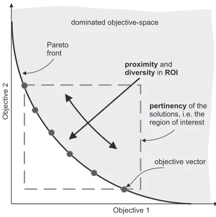
A set of non-dominated solutions1

generated by the op-timiser is known as an approximation set (Zitzler et al., 2003). Three measures of the quality of this approximation set can be considered (Purshouse, 2003). These are illus-trated graphically in Figure. 1, and listed below.

– Proximity. This is a measure of how close the approxi-mation set is to the true Pareto front.

– Diversity. This is a measure of the distribution of the approximation set both in the extent and uniformity of that distribution.

– Pertinency. This criteria measures the relevance of the approximation set to the decision maker (see section 3.4).

Conventional multi-objective optimisation techniques of-ten fail to satisfy these criteria. For example, the goal-attainment method (Gembicki, 1974) and the weighted-sum method (Hwang and Masud, 1979) both only provide single solutions to the optimisation problem - thus failing to provide a diverse distribution of solutions. However, EAs are well suited to this kind of multi-objective optimisation,

1

A solution is termed non-dominated if there is no other solution in the solution set that is superior in all objectives.

Objective 1

Objective2

Pareto front

objective vector

pertinencyof the

solutions, i.e. the region of interest dominated objective-space

proximity

diversity ROI

and in

Fig. 1. The Ideal Solution to a Multi-Objective Optimisation Problem because they search a population of candidate solutions (Deb, 2001). This enables the EA to achieve diversity in its solution-set.

3.3. Many-Objective Optimisation

Theoretical evolutionary multi-objective optimisation (EMO) studies generally consider a small number of ob-jectives, with most of the published literature in the EMO field focussing on the bi-objective case. However, real-world applications of optimisation in engineering design often require a large number of objectives to be dealt with, leading to a growing interest amongst the research com-munity in the area of many-objective optimisation2

. The increased scale of a many-objective optimisation problem means that thepertinency (see Figure. 1) of the candidate solutions, i.e. focussing on those solutions in the decision maker’s region of interest (ROI), is especially important so as to avoid overwhelming the decision maker. This is a major issue because a global trade-off surface for a prob-lem with many conflicting objectives would contain many Pareto-optimal solutions, most of which may not be in the decision maker’s ROI (Purshouse, 2003).

3.4. Decision Making in Engineering Design

The main role of the decision maker in evolutionary multi-objective optimisation is usually to select a single

2

solution from the potentially infinite Pareto-optimal solu-tion set, according to some criteria. In practice the DM is usually only interested in a sub-set of the trade-off surface, thus there is little or no benefit in representing parts of the trade-off surface that lie outside this region of interest. Al-lowing the DM to focus the search on relevant areas of the solution space increases the efficiency of the optimisation process and reduces the amount of irrelevant informa-tion that the DM has to consider (Fleming et al., 2005), thus preventing the DM from becoming overwhelmed (see section 3.3).

DM preferences can be incorporated into the optimisa-tion process in three ways;a posteriori,a priori, and pro-gressively.A posteriori methods of preference articulation involve the DM selecting a compromise solution from the global set of Pareto-optimal solutions.A priori preference articulation and progressive preference articulation aim to achieve a good representation of the trade-off surface in the DM’s ROI. They do this by concentrating the optimiser on a sub-set of the global trade-off surface. Ina priori artic-ulation of preferences the DM expresses their preferences before the start of the optimisation process. However, often the DM may not be sure of their preferences prior to opti-misation, and by stating preferencesa priori the DM may not investigate some areas of the search space that merit attention. A better method is progressive articulation of preferences, where the DM can express preferences during the search and thus incorporate information that becomes available during the search process.

The first scheme for progressive preference articulation in multi-objective evolutionary algorithms was introduced by Fonseca and Fleming (1998). It extended the Pareto-based ranking scheme to allow preferences to be expressed during the run of a multi-objective evolutionary algorithm. These preferences are used in a modified version of dominance which combines Pareto-optimality with a preference opera-tor to rank the candidate solutions in a multi-objective evo-lutionary algorithm. This progressive articulation of pref-erences is a limited form of computational steering. The preferences can be altered during the running of the algo-rithm. However, these are the only variables in the optimi-sation process it is possible to alter.

The ability for the DM to computationally steer the op-timisation routine is desirable due to the large amount of time such optimisation routines often take to complete. By giving the DM the ability to observe the progress of the optimisation process and to alter the parameters as the al-gorithm runs, the DM can act to improve the quality of the solutions produced by this optimisation process. For example, if the optimisation routine is struggling to find solutions of interest to the DM, then the DM could alter the mutation rate, change the bounds on the decision vari-ables, or express design preferences to try to improve the quality of the solutions produced by the algorithm.

4. Implementation

4.1. Steering of the Multi-Objective Evolutionary Algorithm

Before we can implement computational steering in our application, we need to check that the application is ‘able’. In section 2 it was noted that for computational steer-ing to be applied to an application there must be a suitable break-point in its control loop where the program can be interrupted and the steering operations performed.

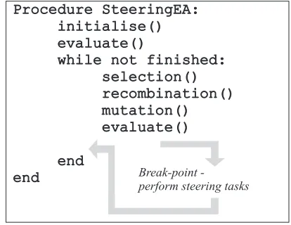
Our optimisation routine contains an ideal break-point due to its iterative nature. This point occurs between the generations of the algorithm, and provides a convenient place to retrieve the current candidate solutions and param-eter set, and to alter those paramparam-eters that are appropriate (see Figure. 2). However, if there are no steering tasks to be performed then the optimisation routine will continue to the next generation.

Procedure SteeringEA: initialise() evaluate()

while not finished: selection() recombination() mutation() evaluate()

end

end Breakpoint

-perform steering tasks

Fig. 2. Pseudo-Code Illustrating the Positioning of a Break-Point in the Control Loop of the Optimiser

Because the next generation of candidate solutions pro-duced by our optimisation routine only relies on the cur-rent generation of candidate solutions and the curcur-rent pa-rameter set it is also simple to implement a checkpointing system. This will take the form of a ‘snap-shot’ of our algo-rithm, taken at the break-point, consisting of the current parameter set and the current generation of candidate so-lutions. If the optimisation routine is to be restored from this point it is a simple matter to reload this ‘snap-shot’ and continue the optimisation process.

solu-tions produced. For example, reducing the exploratory ef-fects of mutation in the algorithm by lowering the mutation rate will reduce the amount of new genetic material com-ing in to the population in each new generation, and thus increase convergence. However this increase in the rate of convergence will come at the risk of converging to a local optimum.

Some other parameters that we can adjust in our steer-ing system are the upper and lower bounds on the deci-sion variables, the population size (either by increasing the number of immigrants or increasing the number of solutions produced by selection), and the fitness assignment method. These parameters all affect the behaviour of the algorithm in different ways. For instance, tightening or loosening the bounds on the decision variables allows the engineer to fo-cus or widen the search in decision space, while increasing the number of immigrants in the population can force the algorithm out of local optima because it introduces new genetic material.

The engineer can alter the probability of a solution being carried over to the next generation by changing the method by which fitness is assigned. For example, if an exponential fitness assignment method is used, then the highest ranked solution will form a proportionally larger part of the next generation compared to a linear fitness assignment method. The second way of steering the optimisation process is to use progressive preference articulation (see section 3.4) to alter the goals and priorities for the objectives, and thus affect the areas of the search space that the algorithm fo-cuses on. The areas of the search space that the algorithm focuses on are defined by the ROI of the DM. This ROI is defined by the preferences specified by the DM, and the al-gorithm focuses on this ROI by assigning a higher rank to those solutions that are in this region. Once a satisfactory value has been achieved for one of the objectives, the objec-tive in question can be constrained to be at least as good as that value. All the potential solutions that do not meet this criterion are ranked worse than those that do, and there-fore the algorithm is steered away from values that violate that constraint. Reducing the region of interest in this way can accelerate the optimisation process and improve the quality of useful solutions.

One possible alternative to computational steering for tuning key parameters in evolutionary computation is the concept of Nested Evolution. This was introduced for a dif-ferential evolution (DE) algorithm in Babu et al. (2004), and consists of an inner optimisation loop and outer opti-misation loop. The inner loop aims to solve the problem, whilst the outer loop optimises the key parameters of the inner loop (with the objective of minimising the number of generation the inner loop runs for). The main drawback of this method is that, as the inner loop is a population based evolutionary optimiser, a large number of function evalu-ations may be needed to tune the key parameters in the

inner loop. Many non-trivial, real-world problems require the use of computationally intensive computer simulations to evaluate the candidate solutions produced by the opti-miser, and it is therefore desirable to keep the number of function evaluations to a minimum. For this reason it was felt that computational steering was a better choice than nested evolution.

4.2. Visualisation

As mentioned in section 2, visualisation is a key compo-nent of computational steering. The visualisation method of any computational steering system must be able to present the user with enough relevant information for the user to guide the process. Therefore, the visualisation method for the intermediate results of our multi-objective evolutionary algorithm must be able to display high-dimensional data sets, as we are dealing with many objectives.

The visualisation of high dimensional data sets in an intuitive manner is extremely difficult. While scatter dia-grams provide a fundamental tool for visualisation of lower dimensional data - allowing the eye to see such features as clustering, outliers and linearity/nonlinearity - they do not generalise easily to more than three dimensions (Wegman, 1990). Many techniques have been proposed to solve this problem (ATKOSoft, 1997), but this paper will focus on two of the most common techniques.

Scatter plot matrices (see Figure. 3) are a commonly used technique in the visualisation of high dimensional data sets. They provide a visualisation technique that facilitates rapid scanning of many dimensions; however discovery of high dimensional patterns can be complicated by the dis-connected representation of multiple aspects of the same point in high dimensional space (Carr et al., 1986). The representational complexity of these scatter plot matrices is high (O(n2

)), because they project n dimensions onto

n×(n−1) scatter plots. This means that this technique

will not scale well to large numbers of variables. This high representational complexity also means that this technique will be unsuitable for on a device with limited screen size, for example that of a PDA.

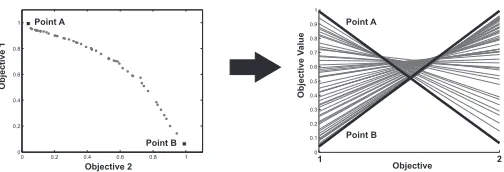
Parallel Coordinate Plots (Inselberg, 1985) are another commonly used technique for visualising high dimensional data. They allow the visualisation of high dimensional data in a simple two dimensional representation. Instead of hav-ing the axes orthogonal to each other, as in Cartesian ge-ometry, the axes are placed in parallel. Thus a point inn

dimensional space will be represented as a line that bisects

MPG

Acceleration

Displacement

Weight

MPG Acceleration Displacement Weight

2000 4000 200 400 10 20 20 40 2000 3000 4000 5000 100 200 300 400 10 15 20 25 10 20 30 40

Fig. 3. A Scatter Plot Matrix Representation of a Four Dimensional Data Set

MPG Acceleration Displacement Weight

−2 −1.5 −1 −0.5 0 0.5 1 1.5 2 2.5 3 Coordinate Value

Parallel Coordinate Plot of Car Features

Fig. 4. A Parallel Coordinate Plot Representing a Four Dimensional Data Set

0 0.2 0.4 0.6 0.8 1 0

0.2 0.4 0.6 0.8

1 Point A

Point B Objective 2 Objective1 1 2 0 0.1 0.2 0.3 0.4 0.5 0.6 0.7 0.8 0.9 1 Point A Point B Objective ObjectiveV alue

Fig. 5. Mapping Between the Cartesian System and the Correspond-ing Parallel Coordinate Plot

Parallel Coordinate plots have a lower representational complexity than scatter plot matrices. The representational complexity of parallel coordinates is O(n) (wherenrefers to the dimensionality of the data), as each line bisecting the axes of the plot represents a single point in high dimen-sional space. Parallel coordinates lose no data in the repre-sentation process; this in turn ensures that there is a unique representation for each unique set of data. The main

weak-nesses of this method are that it requires multiple views to see different trade-offs and it can be difficult to distinguish individual points if many data points are represented.

Parallel Coordinate plots were chosen to perform the vi-sualisation of the data in our computational steering system due to their ease of interpretation and the ability to dis-play all the appropriate data on a screen of limited size, for example on a PDA. To overcome the potential problem of having difficulty distinguishing individual points when the display is cluttered, we will only represent those candidate solutions that fit our modified definition of Pareto optimal-ity (see section 3.4). This will prevent the plot from becom-ing cluttered without removbecom-ing any of the useful data, i.e. the candidate solutions in the ROI of the DM.

4.3. A PDA Implementation

In our application domain of Engineering Design, it would be especially useful for an engineer working on a many-objective optimisation problem to be able to check on the progress of the algorithm from the field. An ideal client for this computational steering system would provide low-cost, portable access to the system.

The implementation of this steering client can be effec-tively realised by using a PDA enabled with a wireless con-nection. The low cost involved in the use of a PDA-based client would allow a wide uptake of this steering system by engineers in the field, whilst the portability of a PDA-based client would enable the engineer to check on the progress of the optimisation routine and alter parameters from any-where with access to the internet. This would be especially useful in the case of a long running optimisation process that may take days to complete.

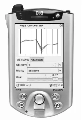
This PDA-based steering system was implemented in two parts. The first part was the design of a steering-enabled multi-objective evolutionary algorithm web service. This service provides the ability to adjust the parameters of the optimisation routine as well as allowing the execution of the multi-objective evolutionary algorithm for a given num-ber of generations. The second part of the implementation was the development of a PDA-based client to interface with the steering-enabled multi-objective evolutionary al-gorithm web service. Due to issues with scarcity of memory and computational power, this client has to be lightweight whilst still providing the desired functionality.

of the objectives (see Figure. 6). The DM can then use this information to improve the optimisation process.

Fig. 6. A PDA Based Implementation of the Steering Client for our Multi-Objective Evolutionary Algorithm

5. Results

A many-objective aircraft controller design problem from literature (Tabak et al., 1979) was chosen to illustrate the computational steering process of the multi-objective evo-lutionary algorithm. This problem involves the design of controller gains to obtain rapid and precise roll response to aileron inputs. There are 8 objectives:

(i) Control Effort

(ii) Bank Angle at 2.8 seconds (iii) Side Slip Deviation (iv) Spiral Root

(v) Roll Damping Root (vi) Dutch Roll Damping Ratio (vii) Dutch Roll Damping Frequency (viii) Bank Angle at 1 second

Firstly we attempted to solve this problem using a multi-objective evolutionary algorithm with common values for the parameters. We ran this algorithm for 100 generations with no preference articulation (see Figure. 7 and Fig-ure. 8). We then reduced the mutation rate and tightened the bounds on some of the decision variables (those that can be seen to contribute to an unsatisfactorily large value for Objective 3) and reran the algorithm (again for 100 gen-erations - see Figure. 9).

Altering the parameters of the multi-objective evolution-ary algorithm improved the results produced by the algo-rithm, but the solutions are still not satisfactory. We then

1 2 3 4 5 6 7 8

−500 0 500 1000 1500 2000 2500 3000

Objective

Standardised Objective Value

Optimisation Results − no preference articulation

Fig. 7. Results of the Initial Execution of the Multi-Objective Evo-lutionary Algorithm

1 2 3 4 5 6 7 8

−20 −10 0 10 20 30 40 50

Objective

Standardised Objective Value

Optimisation Results − no preference articulation

Fig. 8. A Close Up View of the Results of the Initial Execution of the Multi-Objective Evolutionary Algorithm

1 2 3 4 5 6 7 8

−20 −10 0 10 20 30 40 50

Objective

Standardised Objective Value

Optimisation Results − no preference articulation

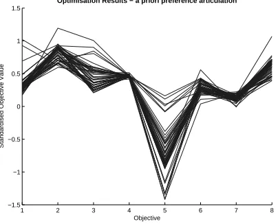
incorporateda prioripreference articulation into the multi-objective evolutionary algorithm (see section 3.4) and ran this MOEA with a priori preference articulation for 100 generations. The results produced by the algorithm witha priori preference articulation are shown in Figure. 10.

1 2 3 4 5 6 7 8

−1.5 −1 −0.5 0 0.5 1 1.5

Objective

Standardised Objective Value

Optimisation Results − a priori preference articulation

Fig. 10. Results of the Multi-Objective Evolutionary Algorithm with

a priori Preference Articulation

As we can see, the incorporation of a priori preference articulation helps the algorithm to achieve better results. This is because the initial preferences given to the algorithm impose a strict ROI (see section 3.4) on which to focus the search. However, these solutions can be further improved by computational steering of the optimisation process. The computational steering of our MOEA was carried out using the steering-enabled web service described in section 4.3, however a desktop implementation of the steering client was used so as to produce the figures in this publication. The results were confirmed using the PDA client.

Figure. 11 is a parallel co-ordinates representation of the 8 objectives after having executed the steering-enabled multi-objective evolutionary algorithm for 20 generations. The dashed line represents the initial goal values for the al-gorithm and therefore the solutions shown on the plot are those that satisfy the initial design specifications, i.e. are within the ROI defined by the DM.

We know from domain knowledge that it is important to keep the control effort (Objective 1) small. This is because high gains can cause sensitivity to sensor noise and may lead to saturation of control actuator response. We will therefore constrain this objective to be at least as good as it is at the moment. This plot also shows that we can tighten the goals on objectives 5, 6, 7, and 8. We then run the multi-objective evolutionary algorithm for another 10 generations (see Figure. 12).

A decision is now made to isolate the best solution (see Figure. 13) with respect to the Roll Damping Root (Objec-tive 5). This objec(Objec-tive is of primary importance for aileron response. We would like to have this objective provide a

1 2 3 4 5 6 7 8

−0.8 −0.6 −0.4 −0.2 0 0.2 0.4 0.6

Objective

Standardised Objective Value

Optimisation Results − after 20 generations

Fig. 11. Results of the Multi-Objective Evolutionary Algorithm after 20 Generations using our Computational Steering Client

1 2 3 4 5 6 7 8

−0.3 −0.2 −0.1 0 0.1 0.2 0.3 0.4 0.5

Objective

Standardised Objective Value

Optimisation Results − after 30 generations

Fig. 12. Results of the Multi-Objective Evolutionary Algorithm after 30 Generations using our Computational Steering Client

fast well damped response. The mutation rate of the multi-objective evolutionary algorithm is then turned down so as to generate multiple solutions that are close to this (see Figure. 14).

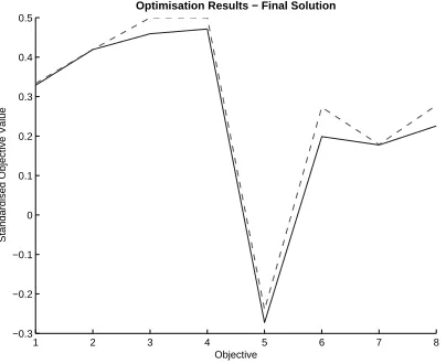
This provides the decision maker with multiple solutions to choose from. The DM then picks the best solution with respect to the Bank Angle at 2.8 seconds (Objective 2) as this ensures that the speed and steadiness of the basic roll response does not drop off with time (see Figure. 15).

6. Conclusions and Further Work

Figure 16 shows the ‘best’ solution produced by each of the runs of the multi-objective evolutionary algorithm3

.

3

1 2 3 4 5 6 7 8 −0.3

−0.2 −0.1 0 0.1 0.2 0.3 0.4 0.5

Objective

Standardised Objective Value

Optimisation Results − after 30 generations

Fig. 13. Isolating a Solution from our Steered Multi-Objective Evo-lutionary Algorithm

1 2 3 4 5 6 7 8

−0.3 −0.2 −0.1 0 0.1 0.2 0.3 0.4 0.5

Objective

Standardised Objective Value

Optimisation Results − after 40 generations

Fig. 14. Results of the Multi-Objective Evolutionary Algorithm after 40 Generations using our Computational Steering Client

1 2 3 4 5 6 7 8

−0.3 −0.2 −0.1 0 0.1 0.2 0.3 0.4 0.5

Objective

Standardised Objective Value

Optimisation Results − Final Solution

Fig. 15. The Final Solution Chosen by Decision Maker from our Steered Multi-Objective Evolutionary Algorithm

The solutions plotted for the first three MOEA runs are those chosen by the decision makera posteriori (see sec-tion 3.4) according to the preferences of the DM. The fourth solution plotted on the graph is the final solution achieved by our computational steering system (see Figure. 15).

1 2 3 4 5 6 7 8

−10 −8 −6 −4 −2 0 2

Objective

Standardised Objective Value

Summary of ‘Best’ Solutions

MOEA run 1 MOEA run 2 ’A Priori’ MOEA Computational Steering

Fig. 16. The Solutions Chosen by the Decision Maker from the Pareto optimal sets produced by each of the MOEAs

As we can see from Figure 16, both of the runs of the MOEA with no preference articulation have produced so-lutions that minimise objective 5 very well. However, this is at the expense of achieving satisfactory values for objective 2 (bank angle at 2.8s) and objective 8 (bank angle at 1s). These objectives are important to ensure a good response from the controller.

The solution selected by the DM from the run of the MOEA witha priori preference articulation is a superior solution (from the DMs point of view) because, although objective 5 is larger, objectives 2 and 8 are much more satisfactory.

The solution achieved using our computational steering system provides the best response of all the solutions. It is the most successful solution in minimising objectives 2 and 8, whilst still achieving good values for the other objectives. Our computational steering system also produced this so-lution in fewer generations than the other MOEA runs (40 generations, compared to 100 generations from each of the other algorithms).

The results produced by computational steering of the optimisation routine are an improvement over those achieved without using steering. This is largely due to the ability to alter the goals progressively. However, being able to alter the mutation rate and other parameters is also an important factor. For instance, in order to pro-duce multiple solutions in close proximity to each other (see Figure. 14), we were able to reduce the mutation rate which decreased the amount of variation produced in the next generation of candidate solutions.

The ability to control the population size of the algorithm also proved useful, as we were able to use large population sizes initially, so as to cover a large area of the search space, and then reduce the population size to allow for quicker execution of the algorithm.

Although altering the bounds on the decision variables was unnecessary in the case of our example, providing the ability to do so is potentially useful. By changing the upper and lower bounds the decision maker is able to guide the search in decision space, as well as guiding the search in ob-jective space using preference articulation. By loosening the bounds on certain decision variables, the DM can expand the search to include previously ignored areas, whereas by tightening the bounds the DM can constrain the area of decision space searched by the optimiser.

This computational steering process for evolutionary op-timisation may allow the user to gain some insight into the optimisation process. As has been noted in the intro-duction to this paper, the evolutionary computation com-munity possesses little more than ‘rules-of-thumb’ when it comes to setting the initial parameters of an evolutionary algorithm (Bullock et al., 2002). By using computational steering of the evolutionary optimisation process, it may be possible to further understand the effects and interac-tions of the different parameters in the algorithm. This is an area for further work.

Acknowledgment

The authors gratefully acknowledge the financial support of the Engineering and Physical Research Council in the UK under Grant Number GR/R67668/01 and input from the engineers at Rolls-Royce Plc and Data Systems & So-lutions.

References

ATKOSoft, 1997. Survey of visuali-sation methods and software tools.

http://europa.eu.int/en/comm/eurostat/research/ supcom.96/30/result/a/visualisation methods.pdf. Babu, B. V., Angira, R., Nilekar, A., 2004. Optimal design

of an auto-thermal ammonia synthesis reactor using

dif-ferential evolution. In: Proceedings of Systemics, Cyber-netics and Informatics (SCI2004). IIIS Press.

Biles, J. A., 2003. Genjam in perspective: A tentative tax-onomy for ga music and art systems. Leonardo: Journal of the International Society for the Arts, Sciences, and Technology 36 (1), 43 – 45.

Brooke, J. M., Coveney, P. V., Harting, J., Jha, S., Pickles, S. M., Pinning, R. L., Porter, A. R., 2003. Computational steering in realitygrid. In: Cox, S. (Ed.), Proceedings of the U.K. e-Science All Hands Meeting.

Bullock, S., Cartlidge, J., Thompson, M., 2002. Prospects for computational steering in evolutionary computation. In: Bilotta, E., Groß, D., Smith, T., Lenaerts, T., Bul-lock, S., Lund, H. H., Bird, J., Watson, R., Pantano, P., Pagliarini, L., Abbass, H., Standish, R., Bedau, M. (Eds.), Artificial Life VIII Workshop Proceedings. MIT Press, pp. 131 – 137.

Carr, D. B., Nicholson, W. L., Littlefield, R. J., Hall, D. L., 1986. Interactive color display methods for multivariate data. In: Wegman, E. J., DePriest, D. J. (Eds.), Statisti-cal Image Processing. Dekker, New York, pp. 215 – 250. Chin, J., Harting, J., Jha, S., Coveney, P. V., Porter, A. R., Pickles, S. M., 2003. Steering in computational science: Mesoscale modelling and simulation. Contempo-rary Physics 44 (5), 417 – 434.

Deb, K., 2001. Multi-Objective Optimization using Evolu-tionary Algorithms. John Wiley and Sons, New York. Farina, M., Amato, P., 2002. On the optimal solution

defini-tion for many-criteria optimizadefini-tion problems. In: Keller, J., Nasraoui, O. (Eds.), Proceedings of the NAFIPS-FLINT International Conference. pp. 233 – 238.

Fleming, P. J., Purshouse, R. C., Lygoe, R. J., 2005. Many objective optimization: An engineering perspective. In: Coello, C. A. C., Aguirre, A. H., Zitzler, E. (Eds.), Pro-ceedings of the International Conference on Evolution-ary Multi-Objective Optimization (EMO2005). Vol. 3470 of Lecture Notes in Computer Science. Springer-Verlag, Berlin, pp. 14 – 32.

Fonseca, C. M., Fleming, P. J., 1998. Multiobjective op-timization and multiple constraint handling with evolu-tionary algorithms - Part I: A unified formulation. IEEE Transactions on Systems, Man, and Cybernetics - Part A: Systems and Humans 28 (1), 26 – 37.

Gembicki, F. W., 1974. Vector optimization for control with performance and parameter sensitive indices. Ph.D. the-sis, Case Western Reserve University, Cleveland, Ohio. Goldberg, D. E., 1989. Genetic Algorithms in Search,

Op-timization and Machine Learning. Addison-Wesley. Hwang, C.-L., Masud, A. S. M., 1979. Multiple Objective

Decision Making - Methods and Applications. Vol. 164 of Lecture Notes in Economics and Mathematical Systems. Springer-Verlag, Berlin.

Johnson, C. R., MacLeod, R., Parker, S. G., Weinstein, D., 2004. Biomedical computing and visualization software environments. Communications of the ACM 47 (11), 64 – 71.

Johnson, C. R., Parker, S. G., Hansen, C., Kindlmann, G. L., Livnat, Y., 1999. Interactive simulation and visu-alization. IEEE Computer 32 (12), 59 – 65.

McCormick, B. H., DeFanti, T. A., Brown, M. D., 1987. Vi-sualization in scientific computing. Computer Graphics 21 (6).

Parker, S. G., Johnson, C. R., Beazley, D., 1997. Compu-tational steering software systems and strategies. IEEE Computational Science and Engineering 4 (4), 50 – 59. Parmee, I., 2002. Improving problem definition through

interactive evolutionary computation. Artificial Intelli-gence for Engineering Design, Analysis and Manufactur-ing 16 (3), 185 – 202.

Purshouse, R. C., 2003. On the evolutionary optimisation of many objectives. Ph.D. thesis, Department of Auto-matic Control and Systems Engineering, University of Sheffield, Sheffield, UK, S1 3JD.

SCIRun, 2006. Scirun: A scientific com-puting problem solving environment. Http://software.sci.utah.edu/scirun.html.

Sims, K., 1991. Artificial evolution for computer graphics. Computer Graphics 25 (4), 319 – 328.

Tabak, D., Schy, A. A., Giesy, D. P., Johnson, K. G., 1979. Application of multiobjective optimization in aircraft control system design. Automatica 15, 595 – 600. Wegman, E. J., 1990. Hyperdimensional data analysis using

parallel coordinates. Journal of the American Statistical Association 85 (411), 664 – 675.