Munich Personal RePEc Archive
Market-based incentives
Grochulski, Borys and Zhang, Yuzhe
Federal Reserve Bank of Richmond, Texas AM University
25 March 2013
Online at
https://mpra.ub.uni-muenchen.de/45576/
Market-based incentives
∗Borys Grochulski† Yuzhe Zhang‡
March 25, 2013
Abstract
We study optimal incentives in a principal-agent problem in which the agent’s outside
option is determined endogenously in a competitive labor market. In equilibrium, strong
performance increases the agent’s market value. When this value becomes sufficiently high,
the threat of the agent’s quitting forces the principal to give the agent a raise. The prospect
of obtaining this raise gives the agent an incentive to exert effort, which reduces the need
for standard incentives, like bonuses. In fact, whenever the agent’s option to quit is close
to being “in the money,” the market-induced incentive completely eliminates the need for
standard incentives.
1
Introduction
The amount of short-term incentives (e.g., bonuses) in compensation packages of many
workers and, especially, executives has attracted a lot of attention and scrutiny in recent years.1
Traditional principal-agent theory provides a rationale for the presence of short-term incentives
in compensation packages: because workers’ actual effort is too costly to monitor and reward
directly, observed performance must be rewarded in order to elicit effort; short-term incentives
∗The views expressed herein are those of the authors and not necessarily those of the Federal Reserve Bank
of Richmond or the Federal Reserve System.
†Federal Reserve Bank of Richmond, [email protected].
‡Texas A&M University, [email protected].
1For example, the Federal Reserve (2011) states that “Risk-taking incentives provided by incentive
compen-sation arrangements in the financial services industry were a contributing factor to the financial crisis that began
are an efficient means of delivering these rewards. Our main result in this paper is that this
rationale does not quite hold once theory recognizes that good to-date performance can boost
a worker’s market value—the value she commands in the labor market if she quits her job. We
introduce a performance-dependent market value to a principal-agent model with limited
com-mitment and show that short-term compensation incentives are usually not needed. Workers’
desire to improve their market value already gives them an incentive, a market-based incentive,
which in a wide range of circumstances is sufficient to elicit effort.
In practice, workers’ consideration for the quality of their future labor market options is an
important source of incentives in numerous occupations ranging from an intern to a tenured
professor. Interns and apprentices work for little or no pay but gain useful skills and experience
that increase the quality of the job they can obtain later. In academia, strong performance in
research or teaching typically is not rewarded with bonuses paid for each publication or for a
high teaching evaluation. Yet, academics work hard to produce strong records of research and
teaching in order to improve their value in the academic labor market. Higher market value
brings quality outside offers that give professors promotions and salary increases in the long run.
In this paper, we capture these forward-looking, market-based incentives in a tractable model
that allows for fully flexible, long-term employment contracts with performance-dependent
com-pensation. In the optimal contract, compensation is downward-rigid and often completely free
of performance-dependent incentives like piece-rate pay or year-end bonuses. Our model
deliv-ers testable predictions on how likely performance-dependent incentives should be observed in
compensation packages of different types of workers.
Market-based incentives arise in our model out of two necessary ingredients. First, workers
have the right to quit at any time. Second, if a worker quits, the value she obtains in the
labor market is higher the stronger her record of to-date performance. The worker’s right to
quit implies that if the market option becomes more attractive to her than her current job,
her employer will have to increase her compensation to match her market value, or she quits.
In either case, the worker benefits when her market value increases. Naturally, this motivates
the worker to boost her market value, which she can do by showing strong performance. Thus,
the worker has an incentive to perform on her current job even if strong performance is not
market value considerations, we will refer to it as a market-based incentive.
Why should a worker’s outside market value increase with stronger on-the-job performance?
In our model, it increases because the worker’s productivity is assumed to be persistent over time
and equally as useful to a potential new employer as it is to her current employer. By putting
in (unobservable) effort on her current job, the worker improves her current productivity, which
benefits her current employer in terms of the increased quantity of output she produces now.
But, because her productivity is persistent, it also makes her more valuable to a potential next
employer. Competition among employers in the labor market translates the next employer’s
higher valuation of the worker into a higher value the worker can obtain by quitting and going
to the market.
It is intuitive that when current effort enhances the worker’s future productivity, fewer
short-term incentives should be necessary because the worker already has some “skin in the game” in
that she benefits when her productivity grows and improves her market value. Since workers’
productivity is persistent in our model, it can be interpreted as human capital. If working hard
on the current job is not only an input into current production but also an investment in the
worker’s (inalienable and transferable) human capital, then it is intuitive that the objectives
of the firm and the worker become better aligned and the need for short-term compensation
incentives decreases.
In our analysis, we make this intuition precise. Formally, we consider a principal-agent
contracting problem in which a risk-neutral firm hires a risk-averse agent/worker whose
pro-ductivity is observable and persistent over time. The evolution of the worker’s propro-ductivity
depends on her effort and exogenous, idiosyncratic shocks, both of which are unobservable. We
embed this contracting problem in a simple model of the labor market, where firms match with
workers frictionlessly. The contract between the firm and the worker specifies compensation
and an effort recommendation for any realization of idiosyncratic shocks to the worker’s
pro-ductivity. The worker can quit at any time and go back to the market. We show that this
right to quit and the persistent impact of the worker’s effort on her productivity (and hence
on her value in the labor market) give rise to a forward-looking, market-based incentive that
encourages effort.
the money.” This is because the firm can provide very limited insurance to the worker if the
worker is about to quit. Limited insurance means the worker’s continuation value is highly
sensitive to the worker’s performance, which gives the worker a strong incentive to exert effort.
The link between the strength of market-based incentives and the worker’s “distance to
default” can be easily seen in the following simple example. Suppose the firm pays the worker
constant compensation for as long as the worker chooses to stay with the firm. How well this
simple contract insures the worker depends on how long the worker stays, which in turn depends
on how good the worker’s market option is. The worse her outside option, i.e., the further away
she is from quitting, the longer the expected duration of this simple contract, and, in effect, the
more insurance this contract provides to the worker. A well-insured worker has little incentive
to put in effort, i.e., the market-based incentive is weak. In particular, if the worker’s market
option is valueless or non-existent, she will never quit, so the simple contract will last forever,
effectively giving the worker full insurance. With full insurance, the worker has absolutely no
incentive to put in effort. In contrast, if the worker’s market option is almost “in the money,”
a very small positive shock to her productivity is enough to elevate her market value above the
value of the simple contract. Since such small shocks happen often, the expected duration of
the simple contract is short and so the contract provides very little insurance to the worker.
With little insurance, the worker’s incentive to put in effort is strong.2
In our model, the worker’s option to quit is formally captured by a participation, or quitting,
constraint. This constraint requires that the worker’s value from the contract with the firm be
at all times at least as large as her market value. How close the worker is to quitting at any given
time (i.e., the worker’s “distance to default”) is measured by how slack the quitting constraint
is. We show that, in line with the intuition from the above simple example, market-based
incentives are strong and standard, contract-based incentives are absent whenever slackness in
the quitting constraint is lower than a threshold. Below this threshold, compensation is constant
whenever the quitting constraint does not bind, and, to keep the worker from leaving, it increases
monotonically whenever the quitting constraint binds.3 Above this threshold, market-based
2Note that it is the upside, not downside, risk that is uninsurable when the insured agent lacks commitment.
3Because there is no economic role for job transitions in our stylized model of the labor market with
homoge-neous firms, we derive the optimal long-term contract under the assumption that workers do not quit if indifferent.
incentives are not strong enough to elicit effort and firms supplement them with some
contract-based incentives, so compensation is not completely independent of current performance. When
slackness in the quitting constraint goes to infinity, the strength of market-based incentives goes
to zero and the optimal contract converges to the solution of the standard principal-agent model
in which there are no market-based incentives.
How frequently market-based incentives are strong in equilibrium depends on how close on
average the quitting constraint is to binding. One important factor determining the average
“distance to default” is the expected change in worker productivity. If productivity tends to
grow over time, the worker’s market value tends to increase, so the quitting constraint binds
often. This makes market-based incentives strong frequently and contract-based incentives
needed rarely. In particular, with a sufficiently large positive trend in worker productivity, the
probability that contract-based incentives are ever used can be arbitrarily small.
We also present an extension of our model in which not only workers but also firms lack
commitment. In particular, firms can fire workers upon incurring a deadweight firing cost. In
this extension, thus, in addition to the worker’s quitting constraint, we have a firm’s
partic-ipation, or firing, constraint. We show that if the firing cost is not too large, the worker is
always exposed to risk and, thus, market-based incentives are always strong. If slackness in the
quitting constraint is low, then, as in our basic model, market-based incentives arise because
the upside risk to the worker’s productivity is uninsurable. If slackness in the worker’s quitting
constraint becomes large, the firm’s firing constraint becomes tight and market-based incentives
arise because the downside risk to the worker’s productivity is not fully insured.
In order to characterize the solution to our model analytically, we make several assumptions
widely used in the dynamic contracting literature. Constant absolute risk aversions (CARA)
preferences and Gaussian shocks let us reduce to one the dimension of the state space sufficient
for a recursive representation of our contracting problem. The optimal contract is then
charac-terized by solving an ordinary differential equation. Although needed for analytical tractability,
these assumptions are not necessary for the existence of market-based incentives. We briefly
consider a version of our model with log preferences and log-normal shocks and show that there,
too, market-based incentives are strong when slackness in the workers’ quitting constraint is
Essential for the existence of market-based incentives are workers’ inability to commit to
staying on the job forever and a positive impact of workers’ on-the-job effort on their market
value. These conditions seem very plausible. The latter condition, in particular, is similar to
learning-by-doing. It will be satisfied whenever putting in effort on the job helps a worker
acquire any kind of skill or experience that is valued in the labor market.
Our characterization of the equilibrium contract gives the following testable predictions of
our model. Performance-based incentives should be more frequently observed (a) in occupations
in which workers do not acquire much general, transferable human capital, (b) when the growth
of a worker’s general productivity is slower, e.g., later in the life-cycle, (c) when firing workers is
costly, and (d) when workers past performance is harder to observe to outsiders. Gibbons and
Murphy (1992), Loveman and O’Connell (1996), and Lazear (2000) provide evidence consistent
with these predictions.
Related literature Market-based incentives are similar to career concerns in that both give
workers a forward-looking motivation for effort. But there are important differences in how
they arise and how they affect workers’ incentives. In the career concerns model of Holmstrom
(1999), workers are risk-neutral, so there is no need for consumption smoothing or insurance.
Workers sell labor services in spot markets every period. Because performance is assumed to be
observable but not contractible, spot wages cannot be made contingent on current performance.
Future spot wages can depend on today’s performance, as the history of performance is available
for each worker. Each period, wages reflect the market’s belief about the worker’s hidden
productivity type. Stronger observed performance improves the market’s expectation of the
worker’s type leading to higher wages in the future. Workers are motivated by career concerns:
they choose effort to manage the market’s assessment of their productivity.
Market-based incentives, by contrast, arise in our model in an environment with risk-averse
workers and risk-neutral firms entering into long-term employment contracts in which
compen-sation can be contingent on current performance. In the optimal long-term contract,
compensa-tion is often insensitive to current performance not because performance is not contractible but
because this way the contract provides maximum feasible consumption smoothing and
insur-ance to the worker. Firms provide incentives mostly through permanent compensation raises
their market value. Since a worker’s productivity is common knowledge at all times, workers
cannot manage market beliefs in our model.
Our paper builds upon two strands of the literature on long-term principal-agent
relation-ships with risk-averse agents: the studies in which the provision of insurance is impeded by
moral hazard, and the studies in which insurance is limited by the lack of commitment. In
the first group, the paper that we are closest to is Sannikov (2008), whom we follow in
study-ing dynamic moral hazard in continuous time.4 Sannikov (2008), however, does not capture
market-based incentives because in his model shocks and actions only affect current output,
and the agent’s outside option is fixed. In our model, shocks and actions have a persistent
effect and, crucially, the agent’s outside option is endogenous and performance-dependent. In
order to obtain a meaningful outside option function, we do not study the optimal contracting
problem in isolation but rather embed it in an simple equilibrium model of the labor market. A
general lesson from the dynamic moral hazard literature is that it is efficient for compensation
to contemporaneously respond to observed performance. With the new elements that we add
to the model, we show the existence of an incentive for effort driven by the agent’s value of
the outside option. This market-based incentive changes the structure of the optimal contract:
compensation responds to performance to a much smaller extent than previous results suggest;
often, it does not respond at all.
Among the numerous studies of optimal contracting subject to limited commitment, our
paper is closely related to Harris and Holmstrom (1982) and Krueger and Uhlig (2006). As in
these studies, we have in our model persistent idiosyncratic shocks, firms/principals that can
commit to long-term contracts, and workers/agents who cannot. This one-sided commitment
friction leads to a downward rigidity in compensation and to limited insurance of the upside risk
in workers’ productivity. While in Harris and Holmstrom (1982) the workers’ outside option is
autarky (spot markets), Krueger and Uhlig (2006) endogenize the outside option by allowing
agents to enter a new long-term contract with another firm after a separation. We follow the
latter approach to modeling the outside option in this paper. Grochulski and Zhang (2011) study
a one-sided limited commitment contracting problem in continuous time and show that the
4Early contributions to the dynamic moral hazard literature include Spear and Srivastava (1987) and Phelan
agent’s continuation value is sensitive to shocks at all times, even when her current consumption
is not. In the present paper, we re-examine these insights in a model that combines the
one-sided commitment friction with moral hazard. We find that, with some qualifications, the
results from the limited-commitment models continue to hold in our more general environment:
wages are downward rigid, the upside risk is not fully insured, and the agent’s continuation
value is sensitive to shocks even if compensation is not. Limited commitment therefore appears
to trump moral hazard considerations in our model: the optimal contract most of the time
looks exactly as if moral hazard were completely absent from the model environment.
There exist a small number of studies that, like we do here, examine optimal contracts under
the two frictions of private information and limited commitment.5 Two studies closely related
to our paper are Thomas and Worrall (1990, Section 8) and Phelan (1995). These papers,
however, do not capture market-based incentives because the agent’s outside option does not
depend on her past performance in the models studied there. In Atkeson (1991), the outside
option of the agent (a borrowing country) does depend on her actions (investment). For this
reason, although that paper asks a different question, we expect that market-based incentives
exist in that environment. However, market-based incentives are probably weak there because
persistence in the impact of the private action (investment) on the value of the outside option
(autarky) is low in that model. In our model, effort has a permanent effect on the worker’s
outside option, which makes market-based incentives much stronger and easier to identify.
Modeling compensation as part of a long-term employment contract has a long tradition in
the economic theory of employment and wage determination that dates back to Baily (1974),
Azariadis (1975), and Holmstrom (1983). Although in this theory, as in our model, employment
contracts provide insurance to workers, shocks considered there are aggregate or
industry-wide, while we consider worker-specific shocks to individual productivity. Also, that literature
abstracts from incentive problems, which are the primary focus of this paper. Our main interest
is in showing the effect of market-based incentives on the structure of the optimal compensation
contract under moral hazard. To this end, we keep the model of the labor market simple. By
assuming frictionless matching between firms and workers, we abstract from search costs and
exogenous separations. All workers in our model economy are employed at all times.
Organization The model environment is formally defined in Section 2. Sections 3 and 4 study
single-friction versions of our model, with full commitment in Section 3 and full information in
Section 4. Optimal contracts from these models serve as benchmarks that we use to solve the
full model in Section 5. In particular, the minimum cost functions from these models provide
useful lower bounds on the cost function in the full model. Section 6 considers robustness of our
results with respect to the functional forms we use as well as with respect to the assumption of
full commitment on the firm side. Proofs of all results formally stated in the text are relegated
to Appendix A.
2
A labor market with long-term contracts
We consider a labor market populated with a large number of agents/workers and a
poten-tially larger number of firms operating under free entry. For concreteness, we will assume that
one firm hires one worker.6 Matching between workers and firms is frictionless: an unmatched
worker can instantaneously find a match with a new firm entering the market. In a newly
formed match, the firm offers to the worker a long-term employment contract. Competition
among firms, those in the market and the potential new entrants, drives all firms’ expected
profits to zero.7
Workers are heterogeneous in their productivity yt, which changes stochastically over time
following a Brownian motion with drift. Letwbe a standard Brownian motionw={wt,Ft;t≥
0} on a probability space (Ω,F,P). A worker’s productivity process y ={yt;t≥0} is y0 ∈R
att= 0 and evolves according to
dyt=atdt+σdwt. (1)
The drift in a worker’s productivity at t, at, is privately controlled by the worker via a costly
action she takes. Specifically, at ∈ {al, ah} with al < ah. The volatility of yt is fixed: σ >0
at allt. Workers are heterogeneous in the initial level of their productivity y0, in the realized
paths of their productivity shocks {wt;t > 0}, and, potentially, in the action path {at;t≥0}
they choose. The path of actions {at;t ≥0} taken by each worker is her private information.
6As long as each worker’s performance is observable, our results would be unchanged if firms in the model
hired multiple workers.
The structure of the productivity process and each worker’s productivity level yt are public
information at all times.
We adopt a simple production function in which the revenue the worker generates for the
firm equals the worker’s productivity yt at all times during her employment with the firm. In
a long-term employment contract, the firm collects revenue{yt;t≥0}and pays compensation
{ct;t ≥0} to the worker. We will identify compensation ct with the worker’s consumption at
allt≥0.8
Formally, a long-term contract a firm and a worker enter att= 0 specifies an action process
a={at;t≥0}for the worker to take, and a compensation/consumption processc={ct;t≥0}
the worker receives. Processes a and c must be adapted to the information available to the
firm.
We assume that firms and workers discount future payoffs at a common rater. In a match,
the firm’s expected profit from a contract (a,c) is given by
Ea
Z ∞
0
re−rt(y
t−ct)dt
,
whereEa is the expectation operator under the action plan a.
Actionatrepresents the worker’s effort at timet. If the worker takes the high-effort action
ah, she improves her current productivity and, hence, the revenue she generates for the firm.
Becauseyt is persistent, high effortah also increases the worker’s expected productivity in the
future. Actionah, however, is costly to the worker in terms of current disutility of effort.
All workers have identical preferences over compensation/consumption processes cand
ac-tion processesa. These preferences are represented by the expected utility function
Ea
Z ∞
0
re−rtU(ct, at)dt
.
To make our model tractable analytically, we will abstract in this paper from wealth effects in
the provision of incentives. That is, we will assume constant absolute risk aversion (CARA)
with respect to consumption by taking
U(ct, at) =u(ct)φ1at=al,
8We can think of the worker’s savings or financial wealth as being observable and thus contractually controlled
where u(ct) =−exp(−ct) < 0, 0 < φ <1, and 1at=al is the indicator of the low-effort action
al at time t. High effort ah is costly to the agent because U(c, ah) =u(c) < u(c)φ =U(c, al)
for all c.9 In Section 6, we discuss the extent to which our results depend on this form of the
utility function.
Firms can commit to long-term contracts, but workers cannot. A worker has the right
to quit and rejoin the labor market at any point during her employment with a firm. In
the market, the worker is free to enter another long-term contract with a new firm. Any
contractual promise by the worker to not use her market option would not be enforceable.
The presence of this inalienable right to quit restricts firms’ ability to insure workers against
the upside risk to their productivity. In particular, contracts will be restricted by workers’
participation (or quitting) constraints defined as follows. Denote by V(yt) the value a worker
with productivityytcan obtain if she quits and rejoins the labor market. This market value will
be determined in equilibrium. We show later (in Proposition 1) that V is strictly increasing.
For a worker with initial productivity y0 ∈ R, a contract (a,c) induces a continuation value
process W={Wt;t≥0} given by
Wt=Ea
Z ∞
0
re−rsU(ct+s, at+s)ds|Ft
. (2)
Contract (a,c) satisfies the worker’s quitting constraints if at all dates and states
Wt≥V(yt). (3)
This constraint is standard in models of optimal contracts with limited commitment (e.g.,
Thomas and Worrall (1988)). It also resembles the lower-bound constraint on the continuation
valueWtused in many principal-agent models with private information (e.g., Atkeson and Lucas
(1995) and Sannikov (2008)), but is in an important way different because the lower bound in
these models is given by some fixed value, whereas in (3) the lower bound V(yt) changes with
the worker’s productivity. Later in the paper we will see that this difference has important
implications for the provision of incentives to the worker at the lower bound.
In this paper, we adopt the convention that when the quitting constraint (3) binds, i.e.,
when the worker is indifferent to quitting, the worker stays. In our model, as in Krueger
9We can equivalently writeU(c
t, at) asu(ct+ 1at=allog(φ
−1)) and interpret log(φ−1)>0 as the consumption
and Uhlig (2006), there are no efficiency gains from separations. Since switching employers
would not make the worker more productive, the best continuation contract that the worker’s
current employer can provide is as good as the best contract that the worker can get in the
market. Adopting the convention that workers do not quit when (3) binds is thus without
loss of generality, but lets us avoid additional notation that would be needed to describe job
transitions.10
Because actionatis not observable, contracts will also have to satisfy incentive compatibility
(IC) constraints. A contract is incentive compatible if no deviation from the recommended
action process a can make the worker better off. We will express IC constraints using the
following results of Sannikov (2008).
Let (a,c) be a contract andWthe associated continuation utility process as defined in (2).
There exists a (progressively measurable) process Y ={Yt;t ≥0} such that the continuation
utility process Wcan be represented as
dWt=r(Wt−U(ct, at))dt+Ytdwta, (4)
where
wta=σ−1
yt−y0− Z t
0
asds
. (5)
Contract (a,c) is IC if and only if for all t and ˜a∈ {ah, al},
r(U(ct,˜a)−U(ct, at)) +σ−1(˜a−at)Yt≤0. (6)
For proof of these results see Sannikov (2008).
In (4),dwa
t =σ−1(dyt−atdt) represents the worker’s current on-the-job performance.
Per-formance attis measured by the change in the worker’s productivity,dyt, relative to what this
change is expected to be at t under the recommended action plan, atdt, and normalized by
σ. Note that as long as the worker follows the recommended action at, her (observable)
per-formancedwa
t will be the same as the (unobservable) innovation term dwt in her productivity
process given in (1).
10If we follow the alternative convention and suppose that the worker quits when (3) binds, the optimal contract
is the same except it ends when (3) binds for the first time and is replaced with a new contract identical to the
continuation of the original contract. This interpretation of long-term contracts is equivalent to the no-separation
Also in (4),Ytrepresents the sensitivity of the worker’s continuation value to current
perfor-mance. Clearly, largerYtwill imply a stronger response ofWtto any given observed performance
dwat. The IC constraint (6) requires that the total gain the worker can obtain by deviating from
the recommended action at to the alternative action ˜abe nonpositive. The first component of
this gain shows the direct impact of the deviation on the worker’s current utility. The second
component shows the indirect impact of the deviation on the continuation utility expressed
as the product of the action’s impact on the worker’s performance and the sensitivity of the
continuation value to performance.
If the recommended action at time tis to exert effort, i.e., ifat=ah, then the IC condition
(6) reduces to ru(ct)(φ−1)≤σ−1(ah−al)Yt, or
Yt
−u(ct) ≥
β, (7)
whereβ=rσa1−φ
h−al >0. Analogously, the low-effort actional is IC att if and only if
Yt
−u(ct) ≤
β.
Written in this form, the IC constraints make it clear that the ratioYt/(−u(ct)) measures the
strength of effort incentives that contract (a,c) provides to the worker at timet. The high-effort
actionahis incentive compatible attif and only if this ratio is greater than the constantβ. Low
effort is incentive compatible if and only if this ratio is smaller than β. As in Sannikov (2008),
higher sensitivity of the worker’s continuation value to her current on-the-job performance,
Yt, makes effort incentives stronger. Due to non-separability of workers’ preferences between
consumption and leisure, the level of consumptionctalso affects the strength of effort incentives
in our model.11 In particular, if the contract recommends high effort, the gain in the flow utility
the worker can obtain by shirking is in our model smaller at higher consumption levels.12 For a
given level of sensitivityYt, thus, higher current consumptionctmakes effort incentives stronger.
11Compare our IC constraint (6) with the IC constraint (21) on page 976 of Sannikov (2008). Consumptionc
t
does not show up in the IC constraint of that model because preferences considered there are additively separable
between consumption and effort.
12This property is particularly easy to see if we interpret log(φ−1)>0 as the consumption equivalent of the
utility the agent gets from shirking. Since shirking at tis equivalent to consumingct+ log(φ−1) instead ofct,
We are now ready to define the contract design problem faced by a firm matched with a
worker. We will define this problem generally as a cost minimization problem in which the firm
needs to deliver some present discounted utility value W ∈[V(y0),0) to a worker whose initial
productivity is y0. Let Σ(y0) denote the set of all contracts (a,c) that at all tsatisfy quitting
constraints (3) and IC constraints (6). The firm’s minimum cost function C(W, y0) is defined
as
C(W, y0) = min (a,c)∈Σ(y0)
Ea
Z ∞
0
re−rt(ct−yt)dt
(8)
subject to W0 =W . (9)
The constraint (9) is known as the promise-keeping constraint: the contract must deliver to
the worker the initial value W. In the special case of W = V(y0), the value −C(V(y0), y0)
represents the profit the firm attains in a match with a worker of typey0 when the worker’s
outside value function isV.
Next, we define competitive equilibrium in the labor market with long-term contracts.
Definition 1 Competitive equilibrium consists of the workers’ market value function V :R→
R− and a collection of contracts (ay0,cy0)
y0∈R such that, for all y0 ∈R,
(i) (ay0,cy0) attains the minimum cost C(V(y
0), y0) in the firm’s problem (8)–(9),
(ii) C(V(y0), y0) = 0 and C(W, y0)>0 for anyW > V(y0).
The first equilibrium condition requires that when firms assume (correctly) that the
work-ers’ outside value is their equilibrium market value, then the equilibrium contracts are
cost-minimizing (i.e., efficient) and in fact deliver to workers their market value. The second
condi-tion comes from perfect competicondi-tion under free entry: profits attained by firms must be zero in
equilibrium and no firm can deliver to a worker a larger value than her market value without
incurring a loss.
2.1 Level-independence of incentives
The following proposition shows a simple relationship between optimal contracts offered
functional form for the equilibrium value function V and gives us a partial characterization of
the cost functionC.
Proposition 1 If (a0,c0) is the optimal contract fory0 = 0, then, for anyy0 ∈R, the optimal
contract(ay0,cy0) is given by
ay0 = a0, (10)
cy0 = c0+y
0. (11)
The equilibrium value functionV satisfies
V(y) =e−yV(0) ∀y∈R. (12)
The minimum cost functionC satisfies
C(W, y) =C(W ey,0) ∀y∈R, W <0. (13)
The independence of the optimal action recommendation from y0, shown in (10), and the
additivity of the optimal compensation plan with respect to y0, shown in (11), follow from
the independence of future productivity changesdytfrom the initial conditiony0 and from the
absence of wealth effects in CARA preferences. With no wealth effects, incentives needed to
induce high or low effort are the same for workers of all productivity levels. The contribution of
changes in a worker’s productivity to a firm’s revenue is also the same for all workers. Thus, the
same effort process is optimally recommended to workers of all productivity levels, and output
produced by a worker with initial productivity y0 =y > 0 is path-by-path larger by exactlyy
than output produced by a worker with initial productivityy0 = 0. Competition among firms
implies then that in equilibrium the worker with y0 = y will obtain the same compensation
process as the worker withy0 = 0 plus the constant amounty at all t.
This structure of the compensation plan allows us to pin down the functional form of the
workers’ market value function V(y0), as given in (12). Intuitively, if a worker with y0 = 0
obtainsV(0) in market equilibrium, then a worker withy0=y will obtaine−yV(0) because her
consumption is larger byyat alltand the utility function is exponential, sou(ct+y) =e−yu(ct)
In addition, this structure of optimal contracts implies a particular form of homogeneity for
a firm’s minimum cost function C(W, y), as shown in (13). Suppose some contract efficiently
delivers some value W < 0 to a worker whose initial productivity y0 = y > 0 (i.e., this
contract attains C(W, y)). Then a modified contract with compensation uniformly decreased
by y will efficiently deliver value eyW < W to a worker whose initial productivity y0 = 0
(i.e., the modified contract will attainC(eyW,0)). But these two contracts generate the same
cost/profit for the firm, as in the second case the worker produces less output (uniformly less
byy) and receives less compensation (also less byy).13
The scalability of the contracting problem and the implied homogeneity of the minimum
cost function greatly simplify our analysis in this paper. In order to solve for the equilibrium,
it is sufficient to find one value,V(0), and one contract that supports it, (a0,c0).
2.2 Optimality of high effort
In our analysis, we will focus on the case in which the recommendation of the high-effort
actionah is optimal and therefore always used by firms in equilibrium. We will verify in Section
5 that the following assumption is sufficient for high effort to be optimal.
Assumption 1 Let κ=σ−2qa2
h+ 2rσ2−ah
. We assume that
κ
1 +κ(ah−al)≥rlog φ −1
+1
2βσ. (14)
The set of parameter values satisfying this assumption is nonempty.14 We will maintain
As-sumption 1 throughout the paper.
2.3 Recursive formulation
In order to find the cost functionC(Wt, yt), we will use the methods of Sannikov (2008) to
study a recursive minimization problem with control variablesat,ut≡u(ct), andYt. Scalability
and homogeneity properties of Proposition 1 let us reduce the dimension of the state space in
13Similarly, a worker with initialy
0=−y <0 will produce and receiveyunits less than a worker withy0= 0.
14Take an arbitrary point in the parameter space and consider decreasing the value ofa
l. Assumption 1 will
eventually hold because loweralmakes a) high effort relatively more desirable, so the left-hand side of (14) grows
this recursive problem. Instead of studying this problem in the two-dimensional state vector
(Wt, yt), we can reduce the state space to a single dimension as follows. Using (13) and (12)
we have
C(Wt, yt) =C(Wteyt,0) =C
Wt
e−ytV(0)V(0),0
=C
Wt
V(yt)
V(0),0
. (15)
This shows that the minimum cost C(Wt, yt) is the same for all pairs (Wt, yt) for which the
ratio Wt
V(yt) is the same. We will find it convenient to transform this ratio further and define a
single state variable as
St≡log
V(yt)
Wt
. (16)
UsingSt, we can express the worker’s quitting constraint (3) as
St≥0, (17)
and the firm’s cost function as
C(Wt, yt) =C
Wt
V(yt)
V(0),0
=C e−StV(0),0
=C(V(St),0),
where the first equality uses (15), the second uses (16), and the third uses (12).15 We will
denote C(V(·),0) by J(·) and solve for this function in the state variable St.
It is useful to note thatSt=u−1(Wt)−u−1(V(yt)), i.e.,Strepresents the difference between
the worker’s continuation value inside the contract and her outside option value when both these
values are converted to permanent consumption equivalents. Indeed, if St = S, the worker is
indifferent between giving up S units of her compensation forever and separating from the
firm.16 BecauseStshows by how much the worker prefers her current contract over the market
option, it represents slackness in the worker’s quitting constraint at timet. LargerStrepresents
larger slackness. In particular, the quitting constraint binds at t if and only ifSt= 0.
With the worker equilibrium value function (12) substituted into (16), we can write the
state variable St as
St=−yt−log(−Wt) + log(−V(0)). (18)
15The IC constraint (7) is not affected by the change of the state variable, as it depends on the control variables
only.
16To see this, note that if S
t = S and {ct+s;s ≥ 0} is a compensation process that gives the worker the
continuation valueWt, then the compensation process{ct+s−S;s≥0}gives the worker the continuation value
Using Ito’s lemma, the law of motion forytgiven in (1), and the law of motion forWtgiven in
(4), we obtain the law of motion for the state variable St under high effort as
dSt= r
−1− ut −Wt +1 2 Yt −Wt 2
−ah
!
dt+
Yt
−Wt −
σ
dwta. (19)
We will find it useful to normalize the control variables ut and Yt by the absolute value of the
worker’s continuation utility. Introducing ˆut≡ −uWtt and ˆYt≡ −YWtt, we express (19) as
dSt=
r(−1−uˆt) +
1 2Yˆ
2
t −ah
dt+Yˆt−σ
dwat. (20)
The Hamilton-Jacobi-Bellman (HJB) equation for the firm’s cost function J is
rJ(St) = rSt−rlog(−V(0)) + min
ˆ
ut,Yˆt
r(−log(−uˆt)) + (21)
J′(S
t)
r(−1−uˆt) +
1 2Yˆ
2
t −ah
+1
2J
′′(S
t)
ˆ
Yt−σ
2
,
where control variables must satisfy ˆYt≥ −uˆtβ to ensure incentive compatibility of the
recom-mended high-effort actionah.
The meaning of the terms in the HJB equation is standard. It may be helpful to write the
HJB equation informally as
rJ(St) = min
r(ct−yt) +J′(St) (drift of St) +
1 2J
′′(S
t) (volatility ofSt)2
. (22)
Intuitively, the first derivativeJ′ represents the firm’s aversion to the drift ofSt because, as we
see in (22), the total costrJ(St) increases byJ′(St) when the drift ofStincreases by one unit.
Similarly, the second derivative J′′ shows how strongly the cost function will respond to an
increase in the volatility ofSt, so in this sense it represents the firm’s volatility aversion. Also,
using definitions of St and ˆut, it is easy to verify that the first three terms on the right-hand
side of (21) represent the firm’s flow costr(ct−yt).
In Section 5, we will characterize optimal long-term contracts by finding a unique solution
to the HJB equation subject to appropriate boundary and asymptotic conditions. In the next
two sections, we provide two important benchmarks by finding optimal contracts in simplified
3
Pay-for-performance incentives in equilibrium with private
information and full commitment
In this section, we will assume full commitment: not only firms but also workers have the
power to commit to never breaking the contract. As in our general model presented in the
previous section, firms match with workers and offer them long-term contracts at t = 0. At
this time, the worker can reject the offer and move to another match instantaneously. Upon
accepting a contract at t = 0, however, the worker commits to not quitting at any t > 0.
This commitment maximizes the match’s surplus as it allows firms to provide better insurance
against fluctuations in workers’ productivity relative to the case in which the workers would
not commit. In particular, it lets firms insure the upside risk to workers’ productivity. We solve
this version of our model in closed form. In equilibrium, firms provide incentives to workers by
making compensation sensitive to current on-the-job performance.
Let ΣF C(y0) denote the set of all contracts (a,c) that at all tsatisfy the IC constraint (6).
The contracting problem we study in this section is identical to the cost-minimization problem in
(8) but with the quitting constraint (3) removed, i.e., with the set of feasible contracts expanded
from Σ(y0) to ΣF C(y0). We will use CF C(W, y0) to denote the minimum cost function in this
problem. The reduced-form cost function JF C(S) is defined analogously. Note that JF C(S) is
defined for anyS, even negative. Market equilibrium is defined as in the general case but using
the cost functionCF C(W, y0) instead of C(W, y0).
The following proposition gives a continuous-time version of standard characterization
re-sults for optimal contracts with private information and full commitment.17
Proposition 2 In the model with full commitment, workers’ equilibrium compensation is given by
ct=y0+
µ+ah
r −µt+ρβw
a
t, (23)
17Spear and Srivastava (1987), Thomas and Worrall (1990), Atkeson and Lucas (1992), and Phelan (1998)
provide characterization results for optimal contracts in discrete-time models with private information and full
commitment, similar to the moral hazard model with full commitment we study in this section in continuous
time. Atkeson and Lucas (1995) and Sannikov (2008) characterize optimal contracts with private information
assuming an exogenous lower bound on the agent’s continuation utility in, respectively, discrete- and
where0< ρ= (p1 + 4r−1β2−1)/(2r−1β2)<1 andµ=r(1−ρ)−1
2ρ2β2>0. The sensitivity
of the equilibrium continuation value Wt with respect to observed performance dwat is
Yt=−u(ct)β at all t. (24)
Proposition 2 shows two main features of optimal compensation schemes in the model with
private information and full commitment: contemporaneous sensitivity of compensation to
performance, represented in (23) by ρβ > 0, and a negative time trend in compensation,
represented in (23) by −µ < 0. The positive contemporaneous sensitivity of compensation
with respect to the worker’s observed performance represents the standard, short-term,
“pay-for-performance” incentive for workers to exert effort. The negative trend in compensation
does not provide effort incentives by itself, but it improves the effectiveness of the
pay-for-performance incentive.
Sensitivity Yt in (24) shows that the IC constraint in (7) binds at all t. This means that
incentives, as measured by the ratioYt/(−u(ct)), are in equilibrium strong enough to make the
recommended high-effort action ah incentive compatible but not any stronger. Incentives are
costly because they reduce insurance. The equilibrium contract is efficient in holding incentives
down to a necessary minimum at all times. Because this minimum does not change over time,
the strength of incentives provided to the worker is always the same in this model.
This section shows that private information requires positive sensitivityYt. The next section
shows that positive sensitivityYtcan arise completely independently of private information: if
workers lack commitment, their productivity shocks cannot be fully insured and, therefore,
their continuation values must remain sensitive to realizations of these shocks. Thus, in an
environment in which private information and limited commitment coexist, limited commitment
potentially could deliver the positive sensitivityYtthat private information requires. Our main
results in this paper, which we give in Section 5, consider precisely this possibility.
4
Market-based incentives in equilibrium with limited
commit-ment and full information
In this section, we discuss the full-information version of our model. As in the general model
worker who has accepted a contract retains the option to quit and go back to the labor market,
where she can find a new match instantaneously. Unlike in the general model, however, we will
assume in this section that workers’ actions on the job are observable, and that workers can
contractually commit to a prescribed course of action.18 The model we study in this section
is essentially a continuous-time version of the Krueger and Uhlig (2006) model with CARA
preferences. This section also generalizes the optimal insurance model studied in Grochulski
and Zhang (2011), where the outside option is assumed to be autarky.
Let ΣF I(y0) denote the set of all contracts (a,c) that at all tsatisfy the quitting constraint
(3). The contracting problem we study in this section is identical to the cost-minimization
problem in (8) but with the IC constraint (7) removed, i.e., with the set of feasible contracts
expanded from Σ(y0) to ΣF I(y0). We will use CF I(W, y0) to denote the minimum cost
func-tion in this problem. The reduced-form cost funcfunc-tion JF I(S) is defined analogously. Market
equilibrium is defined as in the general case but using the cost function CF I(W, y0) instead of
C(W, y0).
Proposition 3 In the model with full information, workers’ equilibrium compensation is given by
ct=mt−ψ, (25)
where mt = max0≤s≤tys and ψ = κσ
2
2r >0. The sensitivity of the continuation value Wt with
respect to observed performance dwa t is
Yt=−u(ct)
κ κ+ 1e
−κ(mt−yt)σ >0. (26)
As in Grochulski and Zhang (2011), the maximum level of productivity attained to date,
mt, is a state variable keeping track of the quitting constraint in this model. The quitting
constraint binds whenever productivity attains a new to-date maximum, i.e., when yt = mt,
and is slack whenever productivity is below its to-date maximum, i.e., when yt < mt. Since
there is no private information and firms and workers discount future payoffs at the same
rate, optimal contracts provide constant compensation (full insurance) to workers whenever
the quitting constraint is slack. When the quitting constraint binds, i.e., when a new to-date
maximum mt is attained, compensation ct increases, as shown in (25). Thus, compensation
never decreases in the full-information model, and it increases faster the faster new maximal
levels of a worker’s productivity are realized.
Since sample paths of the productivity process are continuous, a worker has a better chance
of attaining a new to-date maximum of her productivity—and thus obtaining a permanent
increase in her compensation—the closer her current productivity level yt is to the current
to-date maximum level mt. The worker’s continuation value in the contract, Wt, increases
whenever the chance for the next permanent increase in compensation improves. This means
thatWtincreases when current productivityytincreases, even during time intervals in whichyt
remains strictly belowmt, i.e., when current consumptionct does not at all respond to changes
in yt. This everywhere-positive sensitivity of the continuation value to current performance
is shown in (26). Moreover, (26) shows that the continuation value’s performance sensitivity
Yt increases as the distance between yt and mt decreases. Like St, the distance mt−yt is a
measure of slackness of the quitting constraint (3).19 Thus, sensitivity Yt is larger the closer
the quitting constraint is to binding.
Positive sensitivity Yt >0 arises in this section for reasons completely distinct from those
that give rise to positive sensitivity in the private-information model discussed in the previous
section. There, firms pay for performance in order to elicit high effort. Here, firms can directly
control workers’ effort, but face the possibility of workers quitting. When the quitting constraint
becomes binding, the firm must give the worker a raise in order to retain her. This raise is the
source of positive sensitivity of the continuation value to current performance at all times, even
when the quitting constraint is slack. Because the market option is the source of sensitivityYt
in the model we consider in this section, we will call thisYt market-induced sensitivity.
As we see in the IC constraint (7), incentives are measured in our model by the ratio of Yt
to−u(ct). SensitivityYt is therefore closely related to the notion of incentives. Despite there
being no need for effort incentives in this section, as we assume here that effort is observable
(and thus contractually controllable), we should note that the contract in Proposition 3 does
give the worker an incentive to exert effort because the ratioYt/(−u(ct)) is nonzero under this
19In fact,S
tandmt−yt are related bySt=mt−yt−log
κ+ 1−e−κ(mt−yt)
+ log(κ). Thus,Stis strictly
contract. Indeed, if the firm for some reason neglects to observe and control the worker’s effort
at some instantt, the worker would still choose to supply effort attif the ratioYt/(−u(ct)) she
faces under her contract is larger than β, regardless of what makes this ratio large. Thus, an
effort incentive can exist without private information. Since sensitivity Yt is market-induced,
we will call the effort incentive created byYtthe market-based incentive. The next result shows
that the market-based incentive can be strong in the full-information model.
Corollary 1 The ratio Yt
−u(ct) is strictly decreasing inmt−yt. In particular,
Yt
−u(ct) ≥β if and only if mt−yt≤δ, where δ=κ−1log
κ κ+1
σ β
>0.
This corollary shows that the equilibrium contract obtained in the full-information model
formally satisfies the IC constraint (7) whenever slackness in the quitting constraint (3), as
measured by mt−yt, is small. That means that the market-based incentive is strong in this
region.20 The corollary also shows that the full-information contract is not overall incentive
compatible because it fails to satisfy the IC constraint (7) when the quitting constraint is
suf-ficiently slack. Monotonicity of Yt/(−u(ct)) means that the market-based incentive is stronger
when the quitting constraint is tighter (less slack).
In this section, there is no need for incentives. Yet, they exist in equilibrium as a by-product
of limited commitment. In the next section, we consider the general version of our model with
both moral hazard and limited commitment, where incentives are needed. There, as here,
the market option improves with the worker’s performance, which generates a market-based
incentive. Similar to Corollary 1, the market-based incentive will be strong (sufficient to induce
high effort) when slackness in the quitting constraint is smaller than a threshold. In that region
of the state space, therefore, the equilibrium contract will rely completely on market-based
incentives and will not use pay-for-performance incentives at all.
4.1 Further properties of equilibrium with full information
Proposition 3 describes equilibrium compensation contracts in the full-information model
using two state variables: mtandyt. In Appendix B, we describe the equilibrium of this model
20In particular, the full-information equilibrium contract does satisfy the IC constraint at the onset of every
in terms of the single state variableSt, and characterize the cost functionJF I(St). In particular,
Appendix B discusses the following properties of the equilibrium expressed in terms ofSt. The
drift and the volatility ofStare strictly decreasing inSt. The possibility of violating the quitting
constraint makes the firm infinitely averse to volatility inSt atSt= 0, henceJF I′′ (0) =∞ and
the volatility ofSt atSt= 0 is zero in equilibrium. Equilibrium drift inSt atSt= 0 is strictly
positive (i.e., zero is a reflective barrier for St). In the next section we show that all these
properties continue to hold when both private information and limited commitment are present
in the model.
5
Market-based and pay-for-performance incentives in
equilib-rium with both frictions
In this section, we characterize the optimal contract in our general model, where firms face
both the incentive problem and the quitting constraint.
5.1 Solving the optimal contracting problem
Standard methods for solving second-order differential equations like our HJB equation
(21) require two boundary conditions. Our problem is nonstandard. It has a semi-unbounded
domain (the positive half-line) with only one boundary condition: the second derivative of J
at the boundary St = 0 must be infinite because otherwise the quitting constraint would be
violated immediately after St becomes zero. Despite the lack of a second condition on J at
the boundary, our analysis of the full-information model suggests an asymptotic condition that
can be used to pin down the solution: the cost that the quitting constraint imposes on the
firm must become negligible whenSt goes to infinity because the (time-discounted) chance of
the constraint binding in the future becomes negligible when St is large. When St goes to
infinity, therefore, the cost function in the model with two frictions, J, must converge to the
cost function from the model with private information and full commitment,JF C. In particular,
first derivatives of these functions,J′(S
We will use this asymptotic convergence condition to pin down the solution.21 22
Our analysis of the HJB equation gives the following theorem.
Theorem 1 There exists a unique solution to the HJB equation (21) satisfying the boundary condition J′′(0) = ∞ and the convergence condition limS
t→∞(J′(St)−JF C′ (St)) = 0. This
solution represents the true minimum cost function for the firm.
The method of proof given in Appendix A is similar to that in Sannikov (2008) with two
technical difficulties stemming from the specific boundary and convergence conditions we have.
First, our HJB equation does not satisfy the Lipschitz condition atSt= 0 becauseJ′′(0) =∞.
We overcome this difficulty by using a change of variable technique. Second, the asymptotic
condition requiring convergence ofJ′(St) to J′
F C(St) does not provide an actual restriction on
the boundary of the state space. We overcome this difficulty as follows. We determine a range
of possible values for the first derivative of J at St = 0 and consider a family of candidate
solutions to the HJB equation, one for each possible value ofJ′(0) in this range. We show that
the asymptotic condition requiring thatJ′(St) converge to J′
F C(St) asSt→ ∞ is violated by
all but one candidate solution. We then confirm that the one candidate solution that satisfies
this asymptotic condition indeed represents the true minimum cost functionJ.
Lastly, we verify that the recommendation of high effort is optimal at allt. Lemma A.11 in
the Appendix A shows that this conclusion follows from our Assumption 1.
5.2 Optimality of constant compensation
We now provide the main result of our paper.
21In order to use the cost function J
F C from the one-friction model with full commitment as a benchmark
(lower bound) for J in the two-friction model, one must shiftJF C downward by a constant to account for the
fact that a lower level of utility is provided to the worker in equilibrium in the model with two frictions (the
valueV(0) is lower in this model). It is thus more convenient to express the asymptotic convergence condition in
terms of first derivatives rather than levels because a uniform vertical shift ofJF C does not affect its derivative.
22Appendix B discusses the cost the quitting constraint imposes on the firm in the full-information model
relative to the environment with no frictions (the first best). In that model, this cost does go to zero when
slackness in the quitting constraint goes to infinity: the cost functionJF C and its derivatives converge to the
Proposition 4 In the model with two frictions, there exists a uniqueS∗ >0 such that in each
time interval in which St remains strictly above 0 and below S∗, equilibrium compensation ct
is constant. In the equilibrium contract, the IC constraint (7) binds whenever St ≥S∗, but is
slack whenever St< S∗.
It is a standard result in the literature on optimal compensation that making pay contingent
on current performance is an efficient way of providing effort incentives when the actual effort
of a worker cannot be observed by the firm. That literature, however, assumes that the worker’s
outside option value does not depend on her performance. Our main result shows that when the
worker’s outside option value does depend on her performance, making current pay contingent
on performance may no longer be efficient. In particular, whenever the worker’s market value
is close to the value she obtains by continuing to work for the current employer, optimal
compensation is constant, i.e., completely unresponsive to current performance of the worker,
and the worker chooses to supply effort nevertheless.
Key to this result are two facts. First, as we have seen in Section 4, when the quitting
constraint binds, the firm must increase the worker’s compensation in order to retain her.
Second, when the quitting constraint does not quite bind but is close to binding, the worker’s
effort has a strong impact on the chance that the quitting constraint becomes binding. These
two facts imply that when the worker is close to quitting, she will exert effort in order to actually
hit the quitting constraint and obtain a raise. Knowing this, the firm does not need to provide
an additional incentive via performance-dependent compensation; constant compensation is
efficient.
Proposition 4 also shows that the IC constraint (7) is slack when the quitting constraint (17)
is close to binding. Constant compensation is optimal when St remains in the interval (0, S∗)
precisely because both the quitting and the IC constraint are slack in that region. A slack
IC constraint means that the worker’s incentives are “too strong” (i.e., more than necessary
to induce effort). In fact, when St < S∗ it would be efficient if the firm could provide more
insurance to the worker, thus weakening her incentives, but doing so is impossible due to
the worker’s right to quit. The firm already insures all downside risk to the worker’s future
productivity, but the upside risk is not fully uninsurable. Full insurance is not possible because
her a raise) if her productivity becomes sufficiently high.
When the quitting constraint is relatively slack, St > S∗, the IC constraint binds. This
is because the impact of the worker’s effort on her chance of hitting the quitting constraint is
smaller when the quitting constraint is more distant. The market option still gives the worker
an incentive to supply effort, but this incentive is weak (i.e., not sufficient to induce effort).
The firm must in this case supplement the market-based incentive with a contract-based
pay-for-performance incentive. We study the optimal mix of these incentives in the next section.
In the limiting case with St → ∞, the chance ofSt ever returning to zero becomes negligible
and the strength of market-based incentives goes to zero.
In sum, when St remains below S∗ the optimal contract looks exactly like the optimal
contract from the model with limited commitment and full information in Section 4.23 When
St goes to infinity, in contrast, the optimal contract looks like the optimal contract from the
model with private information and full commitment in Section 3.
5.3 Strength of market-based incentives
In our model, the strength of effort incentives provided to a worker at time t is measured
by the ratio of Yt to −u(ct). Workers will supply effort if and only if this ratio is larger than
β. Proposition 4 shows that in equilibrium, the strength of incentives is only just sufficient
to induce effort when the quitting constraint is relatively slack (St ≥ S∗), but is more than
sufficient when the quitting constraint is relatively tight (St< S∗).
We will now decompose incentives into two parts: forward-looking market-based incentives
and short-term, contract-based incentives. Market-based incentives will be those induced by the
worker’s outside option (as in Section 4). Contract-based incentives will be those not induced
by the market option (as in Section 3). To measure the strength of market-based incentives at
t, we need to compute the ratioYt/(−u(ct)) that the firm would optimally choose at tif limited
commitment were the only friction, i.e., as if the worker’s effort were observable (and hence
controllable) by the firm locally at t. We compute this ratio as follows. Given the optimal cost
23Since workers are hired in our model at market value, i.e., without any slack in the quitting constraint,
optimal compensation for newly hired workers is always free of pay-for-performance incentives. New workers,
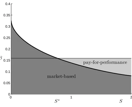
0 1 2 0
0.05 0.1 0.15 0.2 0.25 0.3 0.35 0.4
S S∗
β
market-based
[image:29.612.183.411.108.292.2]pay-for-performance
Figure 1: Composition of incentives
function J, we disregard the IC constraint at t in the HJB equation (21) and use first-order
conditions to obtain current utility u(ct) and sensitivity Yt that the firm would choose in such
a relaxed problem. Denoting the ratio of Yt to −u(ct) from this locally relaxed problem by
˜
Yt/(−u˜(ct)), we have
˜
Yt
−u˜(ct)
= σJ
′(S
t)J′′(St)
J′(St) +J′′(St).
This ratio gives the portion of the actual Yt/(−u(ct)) that is induced by the presence of the
worker’s market option. Thus, it represents the strength of market-based incentives at tin our
model. The remainder of the actualYt/(−u(ct)) represents contract-based incentives that the
firm must inject in order to ensure incentive compatibility of high effort att.
Figure 1 plots the ratio ˜Yt/(−u˜(ct)) against St in a typically parameterized numerical
ex-ample. The strength of market-based incentives decreases as the quitting constraint becomes
more distant. BelowS∗, market-based incentives are strong, meaning they are sufficient to
in-duce effort, i.e., ˜Yt/(−u˜(ct))≥β, and contract-based pay-for-performance incentives are zero.
An implication of strong market-based incentives when St < S∗, as we have seen in
Propo-sition 4, is that compensation is flat and workers provide effort without being compensated
for current performance. AboveS∗, market-based incentives are weak, i.e., not strong enough
to induce worker effort, and the optimal contract supplements them with pay-for-performance
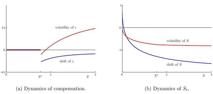
Pay-0 1 2 −0.1
0 0.1
S∗
drift ofc
volatility ofc
S
(a) Dynamics of compensation.
0 1 2
−1 0 1
drift ofS
volatility ofS
S S∗
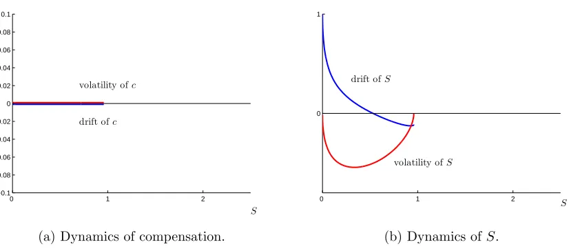
[image:30.612.95.508.101.283.2](b) Dynamics ofSt.
Figure 2: Example withah >0. ThresholdS∗ = 0.76. Stationary point forStis 0.05.
for-performance incentives become stronger as market-based incentives become weaker when
the quitting constraint becomes more slack.
5.4 Dynamics of the equilibrium contract
Unlike the two single-friction models studied in Sections 3 and 4, the model with both
fric-tions does not admit a closed-form solution. In this section, therefore, we describe the dynamics
of the equilibrium contract by characterizing the drift and the volatility of compensationctand
the state variableSt. We provide a mix of analytical and numerical results in this section.
We start out by presenting in Figure 2 the drift and the volatility of ct and St computed
numerically under the parametrization of our model used earlier to produce Figure 1. In panel
(a), we can identify the region of strong market-based incentives by noting that for all St
above zero and below S∗ the drift and the volatility of compensation are both zero, which
means that dct = 0, i.e., compensation remains constant in this region, as predicted earlier
in Proposition 4. WhenSt goes to infinity, the impact of the quitting constraint vanishes and
optimal compensation converges to the optimal compensation from the full-commitment model,
where, by Proposition 2, the drift ofct is−µ <0 and the volatility ofct isρβ >0.
In addition to these properties of compensation at low and high values of the state variable,