http://www.scirp.org/journal/am ISSN Online: 2152-7393
ISSN Print: 2152-7385
Optimum Control for Spread of Pollutants
through Forest Resources
Nita H. Shah
*, Moksha H. Satia, Bijal M. Yeolekar
Department of Mathematics, Gujarat University, Ahmedabad, India
Abstract
Pollution has become the most critical factor spread by forest resources through wood-based and non-wood based industries. In other words, pollu-tion is omnipresent. In this paper, the major pollutants caused due to wood and non-wood based industries are discussed which are the primary resources of the forest in spreading the pollution. In order to study the impact of indu-strialization and associated pollution on forest resources, the system of non-linear ordinary differential equations is formulated. The controls are ad-vised on both types of industries to reduce the pollution.
Keywords
Mathematical Model, Pollutants, Pollution, Forest Resources, Wood and Non-Wood Based Industries,
System of Non-Linear Ordinary Differential Equation, Control
1. Introduction
The forest resources mean a large area covered by trees. It means the various types of vegetation automatically growing on forest land where forest is consi-dered as if it grew trees in the past, or will grow trees in the future. Wood-based industries are the branch of production and employment based on the fabrica-tion, processing and preparation of products from raw materials and merchan-dises of wood and wood-based pulp products. Non-wood based industries are the branch of production and employment based on fabrication, processing and preparation of products from water, energy, chemicals etc. The term “pollution” is a substance into the environment which has harmful or poisonous effects on living beings. “Pollutants” are the components of pollution. It is observed that most of the pollution is associated with man-made industries. Wood and non- wood based industries affect the environment through pollutants emitted from How to cite this paper: Shah, N.H., Satia,
M.H. and Yeolekar, B.M. (2017) Optimum Control for Spread of Pollutants through Forest Resources. Applied Mathematics, 8, 607-620.
https://doi.org/10.4236/am.2017.85047
Received: March 16, 2017 Accepted: May 12, 2017 Published: May 15, 2017 Copyright © 2017 by authors and Scientific Research Publishing Inc. This work is licensed under the Creative Commons Attribution International License (CC BY 4.0).
http://creativecommons.org/licenses/by/4.0/
them merged in air as well as absorbed by forest region can be harmful for na-ture and can kill human organisms, essential microbes etc.
The forest resources are significant for human and some organisms. But after industrial revolution in 18th century, industries are also growing very speedy [1]. This growth of wood and non-wood based industries has reduced the density of forest region. Damodar Valley, Nowamundi, Saranda are example of reduced forest resources [2]. Once Damodar Valley was covering 65% of forest area, now-a-days it is surrounded by only 0.05% [3]. In past, few years, the tempera-ture of the environment is increasing due to the emission of pollutants which is examined by scientists and ecologists. This gives opposite impact on humans and environment [4][5]. Absorption of pollutants by the plants is harmful and which affected the growth of forest resources [6][7][8][9].
This motivated to formulate the system in which the effect of industrialization on the forest resources is analyzed. Some researchers have studied the mathe-matical model for the effects of industrialization and pollution on forest re-sources. [10] studied the models for the effect of toxicant in single-species and predator-prey system. [11] analysed the modeling effect of an intermediate toxic product formed by uptake of a toxicant on plant biomass. [12] introduced the effects of industrialization and pollution on resource biomass with the help of a mathematical model. [13] have performed the modeling effects of industrializa-tion, population and pollution on renewable resources. [14] deliberated model-ing effects of primary and secondary toxicants on renewable resources.
In this paper, a mathematical model is formulated with hereditary transmis-sion of SIRS model in Section 2. The stability analysis of the transmistransmis-sion model is derived in Section 3. Sensitivity analysis is carried out in Section 4. Optimal control for the forest resources is discussed in Section 5. In Section 6, the model validated with numerical simulation and analysis.
2. Mathematical Modeling
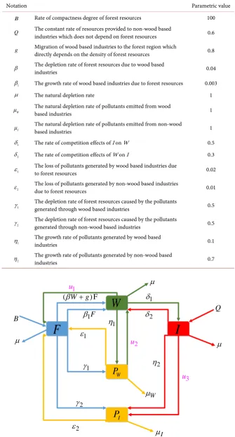
In the society, there are different types of industries and pollution. Everybody in the society plays a role to decrease the pollution. Therefore, in the proposed model, five discrete compartments viz. the density of forest resources (F), the density of wood based industries (W), the density of non-wood based industries (I), the pollutants through wood based industries (PW) and the pollutants through non-wood based industries (PI) are considered. u1 is the rate which de-creases wood based industries to control the usage of forest resources. u2 and u3 are the control rates which decreases pollutants due to wood and non-wood based industries, respectively.
The notations and parametric values for the dynamical model are exhibited in
Table 1.
Using these notations and assumptions which are required for formulating the mathematical model, the transmission diagram of forest resources is shown in
Figure 1.
Table 1. Notation and parametric values.
Notation Parametric value
B Rate of compactness degree of forest resources 100 Q The constant rate of resources provided to non-wood based
industries which does not depend on forest resources 0.6 g Migration of wood based industries to the forest region which
directly depends on the density of forest resources 0.8 β The depletion rate of forest resources due to wood based
industries 0.04
1
β The growth rate of wood based industries due to forest resources 0.003
µ The natural depletion rate 1
W
µ The natural depletion rate of pollutants emitted from wood
based industries 1
I
µ The natural depletion rate of pollutants emitted from non-wood
based industries 1
1
δ The rate of competition effects of I on W 0.5
2
δ The rate of competition effects of W on I 0.3
1
ε The loss of pollutants generated by wood based industries due
to forest resources 0.02
2
ε The loss of pollutants generated by non-wood based industries
due to forest resources 0.01
1
γ The depletion rate of forest resources caused by the pollutants
generated through wood based industries 0.5
2
γ The depletion rate of forest resources caused by the pollutants
generated through non-wood based industries 0.5
1
η The growth rate of pollutants generated by wood based
industries 0.1
2
η The growth rate of pollutants generated by non-wood based
industries 0.7
F
W
I
W
P
I
P
1
δ
(
β
W
+
g
) F
2
δ
Q
1
γ
2
γ
µ
WI
µ
1F
β
µ
B
1
u
µ
µ
1η
2
η
1ε
2
ε
2
u
3
[image:3.595.204.540.90.714.2]u
industries with associated pollutants is described as follows:
(
)
1 1 1 2 2 1d
d W I
F
B W g F FW P F F P u W F
t = − β + −β +ε −γ −γ +ε + −µ (1)
(
)
1 1 2 1 1 2d d
W
W g F FW W I W u W u W W
t = β + +β −δ +δ −η − − −µ (2)
1 2 2 3
d d
I
QI W I I u I I
t = +δ −δ −η − −µ (3)
1 1 1 2
d d
W
W W W
P
W P F u W P
t =η −ε +γ + −µ (4)
2 2 2 3
d d
I
I I I
P
I P F u I P
t =η −ε +γ + −µ (5) Equations (1) to (5) is described as system (1) in the model.
With F+W + +I PW +PI =N and F>0;W I, ≥0;Pw≥0;PI ≥0
Adding all the above system of differential equations gives,
(
)
(
)
d
0 dt F+W+ +I PW +PI = +B QI−µ F+W+I −µWPW −µIPI ≥ (6) This gives,
(
)
lim sup W I
t
B
F W I P P
µ
→∞ + + + + ≤ (7)
Therefore, the feasible region for system (1) is
(
F W I PW PI)
F W I PW PI B,F 0;W I P P, , W, I 0µ
Λ = + + + + + + + + ≤ > ≥
. (8)
Thus, the equilibrium state of the system (1) is 0 , 0, 0, 0, 0
B X
µ
= Next, the basic reproduction number R0 can be calculated using the next generation matrix.
Let X′ =
(
W F I P, , , W,PI)
′, where dash denotes derivative. So,( )
( )
d d
X
X X V X
t
′ = = − (9)
where
( )
X denotes the rate of appearance of new individual in compart-ment and V X( )
represents the rate of transfer of culture, which is given by( )
(
)
( )
1
1 2 1 1 2
1 1 1 2 2 1
1 2 2 3
1 1 1 2
2 2 2 3
0 , 0 0 0 W I
W W W
I I I
FW
X
gF W I W u W u W W
B WF gF WF P F F P u W F
V X QI W I I u I I
W P F u W P
I P F u I P
β β
δ δ η µ
β β ε γ γ ε µ
δ δ η µ
η ε γ µ
η ε γ µ
Now,
( )
0( )
01 2 0 0 , 0 0 v f
D X DV X
J J = =
where f and v are 5 5× matrices defined as
( )
0 ,( )
0i i
j j
X V X
f v X X ∂ ∂ = = ∂ ∂
(
)
(
)
11 1 1 2 2
1
1 1 2 1 2
1 2 2 3
1 2 1 1
2 2 3 2
0 0 0 0 0 0 0 0 0
, 0 0 0 0 0 0 0 0 0 0 0 0 0 0 0
0 0 0
0 0 0
0 0 0 0 W I B f
u u g
B u g v Q u u u β β µ
δ η µ δ
β β
γ γ µ ε ε
µ
δ δ η µ
η γ ε µ
γ η ε µ
+ = + + + + − − + − + + + − − = − − + + + + − − − + − − − +
Here, v is non-singular matrix, so the basic reproduction number R0 is
1 0 spectral radius of matrix .
R = fv− (10)
(
)
(
)
(
)(
1 1 1 1 2)
2 1 1(
1 2 2)
0
1 1 1 2 1 1 2 2 1 1 1 2 2 2 1 1 2 2 1 1 2 3 1 2 1
BC B D D D D
R
A C B D D D D g A C D D C D A C D
β β γ ε γ ε
µ δ δ γ ε γ ε δ ε ε
+ − −
=
− − − + + +
(11)
where
(
1)
1 1 1 1 2 , 2 1, 3 1 2, 1 1 2 ,
B
A δ η u u µ A β β u A η u B g γ γ µ
µ +
= + + + + = − = − − = + + +
1 2 2 3 , 2 2 3, 1 1 w, 2 2 I
C = − +Q δ +η +u +µ C = − −η u D =ε +µ D =ε +µ
In next section, equilibrium of the forest resources transmission model is dis-cussed.
3. Equilibrium
The equilibrium for the local and global stability of the forest transmission mod-el are discussed here.
3.1. Local Stability
The forest resources equilibrium is locally asymptotically stable if all the eigen-values of the matrix have positive real eigen-values [15]. The Jacobian matrix for sys- tem (1) at 0 , 0, 0, 0, 0
B X
µ
=
(
)
(
)
1 2 1 1 1 2
1 1 1 1 2 2
1 2 2 3
1 1 2 1
2 2 3 2
0
0 0
0 0 0
0 0
0 0
W
I
B
g u
B
g u u
J
Q u
u
u
γ γ µ β β ε ε
µ
β β δ η µ δ
µ
δ δ η µ
γ η ε µ
γ η ε µ
− − − − − + +
+ − − − − −
=
− − − −
+ − −
+ − −
Using the parametric values given in the Table 1,
( )
(
1)
1 2(
1)
1 1 22 1 2 1 2 3 3 W I 6.97 0
trace J g W F Q
u u u
β β γ γ β β δ η δ
η ε ε µ µ µ
= − − + − − + + − − + −
− − − − − − − − − = − < (12)
Hence, system (1) is locally stable.
3.2. Global Stability
The forest resources transmission model is globally stable is
(
1)
det I− fv− >0.
(
1)
0
det I− fv− = −1 R = −1 0.4960=0.5040>0 (13)
Therefore, system (1) is also globally stable.
4. Sensitivity Analysis
In this section, the sensitivity analysis for all parameters are discussed in Table 2.
The normalised sensitivity index of the parameters is computed by using the following formula: 0 0
0
R R
R α
α α ∂
ϒ = ⋅
∂ where α denotes the model parameter.
[image:6.595.207.538.581.734.2]The rate of compactness degree of forest resources, the constant rate of re-sources, migration of wood based industries to forest region, the depletion rate of forest resources due to wood based industries, the growth rate of wood based industries due to forest resources, the rate of competitive effects of I on W, the loss of pollutants generated by wood based industries due to forest resources, the loss of pollutants generated by non-wood based industries due to forest re-sources and the growth rate of pollutants generated by wood based industries
Table 2. Sensitivity analysis.
Parameter Value Parameter Value
B + δ1 +
Q + δ2 -
g + ε1 +
β + ε2 +
1
β + γ1 -
µ - γ2 -
W
µ - η1 +
I
have positive effect on R0 which means they are helping us to save forest re-sources. Other parameters have negative impact on model.
5. Optimal Control
The objective of the model is to minimize the number of pollutants through wood and non-wood based industries to revive forest resources. The control functions are united to achieve the objective. The objective function for the ma-thematical model of forest resources in system (1) along with the optimal control is given by
(
)
(
2 2 2 2 2 2 2 2)
1 2 3 4 5 1 1 2 2 3 3
0
, d
T
i W I
J u Ω =
∫
A F +A W +A I +A P +A P +w u +w u +w u t (14)where, Ω denotes set of all compartmental variables, A A A A A1, 2, 3, 4, 5 denote non-negative weight constants for F W I P, , , W,PI compartments respectively and w w w1, 2, 3 are weight constants for control variables u u u1, 2, 3 respectively. As, the weight parameters w w1, 2 and w3 are constants of forest resources control
( )
u1 , wood based industries control( )
u2 and non-wood basedindus-tries
( )
u3 , from which the optimal control condition is normalized. u1 is the control variable for minimizing the use of forest resources. u2 and u3 are the control rates which minimize the density of wood and non-wood based indus-tries respectively which automatically reduce the pollutants also. To compute the values of control variables u u1, 2 and u3 from t=0 to t=T such that( ) ( ) ( )
(
)
{
(
*)
(
)
}
1 , 2 , 3 min i , / 1, 2, 3
J u t u t u t = J u Ω u u u ∈φ (15)
where
φ
is a smooth function on the interval[ ]
0,1 . The optimal controls de-noted by *, 1, 2, 3
i
u i= are found by accumulating all the integrands of Equation (14) using the lower bounds and upper bounds respectively with the results of
[16].
Now, using the pontrygin’s principle from [17], to minimize the cost function in (14) by constructing Lagrangian function consisting of state equations and adjoint variables Ai=
(
λ λ λ λ λ
1, 2, 3, 4, 5)
as(
)
(
)
(
)
(
)
(
)
(
)
(
)
(
)
2 2 2 2 2 2 2 2
1 2 3 4 5 1 1 2 2 3 3
1 1 1 1 2 2 1
2 1 1 2 1 1 2
3 1 2 2 3
4 1 1 1 2
5 2 2 2 3
, i W I
W I
W W W
I I I
L A A F A W A I A P A P w u w u w u
B W g F FW P F F P u W F
W g F FW W I W u W u W W
QI W I I u I I
W P F u W P
I P F u I P
λ β β ε γ γ ε µ
λ β β δ δ η µ
λ δ δ η µ
λ η ε γ µ
λ η ε γ µ
Ω = + + + + + + +
+ − + − + − − + + − + + + − + − − − − + + − − − − + − + + − + − + − − (16)
The partial derivative of the Lagrangian function with respect to each variable of the compartment gives the adjoint equation variables Ai=
(
λ λ λ λ λ
1, 2, 3, 4, 5)
corresponding to the system (1) which is as follows:
(
)(
) (
)
(
)
(
)
1 1 1 2 1 2 1
1 4 1 1 5 2 1
2
L
W F W g W
F
λ λ λ β λ λ β
λ λ γ λ λ γ µλ
(
)
(
)
(
)
(
)
(
)
(
)
2 2 1 2 1 2 1 2 1 1
2 3 1 2 4 1 2 4 2 2
2
L
W W F F u
W
u
λ λ λ β λ λ β λ λ
λ λ δ λ λ η λ λ µλ
∂ = − = − + − + − + − ∂ + − + − + − + (18)
(
)
(
)
(
)
33 3 2 2 3 5 3 3 5 2 3 3
2
L I
W I u Q
λ
λ λ δ λ λ λ λ η λ µλ
∂ = − ∂ = − + − + − + − + + (19)
(
)
4 2 4 W 4 1 1 W 4
W
L
W P P
λ
= − ∂ = − +λ
−λ ε
+µ λ
∂
(20)
(
)
5 2 5 I 5 1 2 I 5
W
L
W P P
λ
= − ∂ = − +λ λ ε
− +µ λ
∂
(21)
The necessary condition for Lagrangian function L to be optimal for controls are
(
)
1 6 1 2 1
1
2 0
L
u W u W
u
λ
λ
∂
= − = − + − =
∂
(22)
(
)
2 7 2 2 4
2
2 0
L
u W u W
u
λ λ
∂
= − = − + − =
∂
(23)
(
)
3 6 3 3 5
3
2 0
L
u W u I
u
λ λ
∂
= − = − + − =
∂
(24)
To find the values of u u1, 2 and u3 solve Equations (22), (23) and (24) then
(
2 1)
1 6 2 W u W
λ λ
−= ,
(
2 4)
2 7 2 W u W
λ
−λ
= and
(
3 5)
3 6 2 I u W
λ λ
−= (25)
Thus, the required optimal control condition is computed as
(
2 1)
1 1 1
6
max , min , 2
W
u a b
W
λ λ
∗= −
(26)
(
2 4)
2 2 2
7
max , min , 2
W
u a b
W
λ λ
∗= −
(27)
(
3 5)
*3 3 3
6
max , min , 2
I
u a b
W
λ λ
−
=
(28)
In next section the optimal control is calculated numerically to support the analytical results.
6. Numerical Simulation
Using the data given in Table 1 and Table 2, the sensitivity on model parame-ters is carried out.
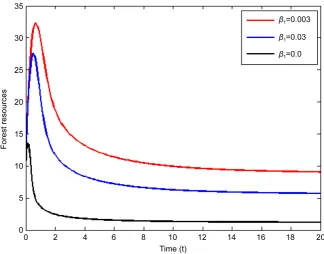
The Figure 2 specifies that as the depletion rate of forest resources due to wood based industries increases the density of forest resources decreases.
From Figure 3, it is observed that increase in growth rate of wood based in-dustries due to forest resources the density of forest resources decreases.
Figure 2. Effects of the depletion rate of forest resources due to wood based industries on forest resources.
Figure 3. Effects of the growth rate of wood based industries due to forest resources on forest resources.
From Figure 5 it is concluded that as the constant rate of resources provided to non-wood based industries increases the forest resources decreases.
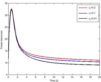
[image:9.595.211.536.375.629.2]Figure 4. Effects of the loss of pollutants generated by non-wood based industries on for-est resources.
Figure 5. Effect of the constant rate of resources provided to non-wood based industries on forest resources.
[image:10.595.210.537.381.642.2]With control forest resources degradation reduces at a lower rate compare to no effective majors are taken up as shown in Figure 7.
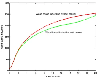
[image:11.595.208.539.168.717.2]Figure 8 suggest that wood based industries can be controlled with effective majors at a lower rate compare to no control over it and when control is applied to wood based industries it decreases by 7%. Similar observation is from Figure 9 for non-wood based industries. In fact, it decreases by 4%.
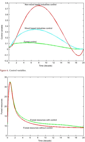
Figure 6. Control variables.
Figure 8. Wood based industries with control and without control.
Figure 9. Non-wood based industries with control and without control.
7. Conclusions
the density of forest resources. The wood-based industries reduce the density of forest resources directly by harvesting as well as indirectly by pollutants. But non-wood based industries reduce the density of forest resources only indirectly by pollutants. Therefore, by more industries the forest resources are affected and may be wiped out.
The stability of forest resources model discussed with numerical data. The ba-sic reproduction number is computed as 0.4960, which shows that controls on construction of wood and non-wood based industries will be beneficial to reduce the pollution. This suggested growing more and more forest resources and putting up less number of industries per human usage.
Acknowledgements
Authors sincerely thank for the constructive comments of the reviewers. The authors thank DST-FIST file # MSI-097 for technical support to the department.
References
[1] Dubey, B., Sharma, S., Sinha, P. and Shukla, J.B. (2009) Modeling the Depletion of Forestry Resources by Population and Population Pressure Augmented Industriali-zation. AppliedMathematicalModeling, 33, 3002-3014.
[2] Lata, K., Dubey, B. and Misra, A.K. (2016) Modeling the Effects of Wood and Non- Wood Based Industries on Forestry Resources. NaturalResourceModeling, 29, 559- 580. https://doi.org/10.1111/nrm.12111
[3] Priyadarshi, N. (2010) Effects of Mining on Environment in the State of Jharkhand, India-Mining Has Caused Severe Damage to the Land Resources.
[4] Intergovernmental Panel on Climate Change (2014) Climate Change 2014-Impacts, Adaptation and Vulnerability: Regional Aspects. Cambridge University Press, Cambridge, 1-32.
[5] Patwardhan, A., Semenov, S., Schnieder, S., Burton, I., Magadza, C., Oppenheimer, M. and Sukumar, R. (2007) Assessing Key Vulnerabilities and the Risk from Cli-mate Change. In: ClimateChange, 779-810.
[6] Chappelka, A.H. and Samuelson, L.J. (1998) Ambient Ozone Effects on Forest Trees of the Eastern United States: A Review. NewPhytologist, 139, 91-108.
https://doi.org/10.1046/j.1469-8137.1998.00166.x
[7] Davison, A.W. and Barnes, J.D. (1998) Effects of Ozone on Wild Plants. New Phy-tologist, 139, 135-151. https://doi.org/10.1046/j.1469-8137.1998.00177.x
[8] Treshow, M. (1968) Impact of Air Pollutants on Plant Populations. Phytopathology 58, 8.
[9] Treshow, M. (1984) Air Pollution and Plant Life.
[10] Freedman, H.I. and Shukla, J.B. (1991) Models for the Effect of Toxicant in Single- Species and Predator-Prey Systems. JournalofMathematicalBiology, 30, 15-30.
https://doi.org/10.1007/BF00168004
[11] Naresh, R., Sundar, S. and Shukla, J.B. (2006) Modeling the Effect of an Interme-diate Toxic Product Formed by Uptake of a Toxicant on Plant Biomass. Applied MathematicsandComputation, 182, 151-160.
[12] Dubey, B., Upadhyay, R.K. and Hussain, J. (2003) Effects of Industrialization and Pollution on Resource Biomass: A Mathematical Model. EcologicalModeling, 167, 83-95.
[14] Shukla, J.B., Agrawal, A.K., Sinha, P. and Dubey, B. (2003) Modeling Effects of Pri-mary and Secondary Toxicants on Renewable Resources. NaturalResource Model-ing, 16, 99-120.
[15] Al-Amoudi, R., Al-Sheikh, S. and Al-Tuwairqi, S. (2014) Qualitative Behavior of Solutions to a Mathematical Model of Memes Transmission. InternationalJournal ofAppliedMathematicalResearch, 3, 36-44.
[16] Fleming, W.H. and Rishel, R.W. (2012) Deterministic and Stochastic Optimal Con-trol. Vol. 1, Springer Science & Business Media, New York.
[17] Pontriagin, L.S., Boltyanskii, V.G., Gamkrelidze, R.V. and Mishchenko, E.F. (1986) The Mathematical Theory of Optimal Process. Gordon and Breach Science Pub-lishers, New York, 4-5.
Submit or recommend next manuscript to SCIRP and we will provide best service for you:
Accepting pre-submission inquiries through Email, Facebook, LinkedIn, Twitter, etc. A wide selection of journals (inclusive of 9 subjects, more than 200 journals) Providing 24-hour high-quality service
User-friendly online submission system Fair and swift peer-review system
Efficient typesetting and proofreading procedure
Display of the result of downloads and visits, as well as the number of cited articles Maximum dissemination of your research work
Submit your manuscript at: http://papersubmission.scirp.org/