http://wrap.warwick.ac.uk/
Original citation:
Yuan, Ke, Girolami, Mark, 1963- and Niranjan, Mahesan (2012) Markov chain Monte
Carlo methods for state-space models with point process observations. Neural
Computation, Volume 24 (Number 6). pp. 1462-1486. ISSN 0899-7667
Permanent WRAP url:
http://wrap.warwick.ac.uk/64698
Copyright and reuse:
The Warwick Research Archive Portal (WRAP) makes this work by researchers of the
University of Warwick available open access under the following conditions. Copyright ©
and all moral rights to the version of the paper presented here belong to the individual
author(s) and/or other copyright owners. To the extent reasonable and practicable the
material made available in WRAP has been checked for eligibility before being made
available.
Publisher statement:
© 2012 The MIT Press
Link to the journal's homepage:
http://www.mitpressjournals.org/doi/abs/10.1162/NECO_a_00281#.VIbjaTGsV8E
Copies of full items can be used for personal research or study, educational, or
not-for-profit purposes without prior permission or charge. Provided that the authors, title and
full bibliographic details are credited, a hyperlink and/or URL is given for the original
metadata page and the content is not changed in any way.
A note on versions:
The version presented in WRAP is the published version or, version of record, and may
be cited as it appears here.
Markov Chain Monte Carlo Methods for State-Space
Models with Point Process Observations
Ke Yuan
School of Electronics and Computer Science, University of Southampton, Southampton, SO17 1BJ, U.K.
Mark Girolami
Department of Statistical Science, Centre for Computational Statistics and Machine Learning, University College London, London,
WC1E 6BT, U.K.
Mahesan Niranjan
School of Electronics and Computer Science, University of Southampton, Southampton, SO17 1BJ, U.K.
This letter considers how a number of modern Markov chain Monte Carlo (MCMC) methods can be applied for parameter estimation and inference in state-space models with point process observations. We quantified the efficiencies of these MCMC methods on synthetic data, and our results suggest that the Reimannian manifold Hamiltonian Monte Carlo method offers the best performance. We further compared such a method with a previously tested variational Bayes method on two experimental data sets. Results indicate similar performance on the large data sets and su-perior performance on small ones. The work offers an extensive suite of MCMC algorithms evaluated on an important class of models for physi-ological signal analysis.
1 Introduction
Latent processes in the brain during the processing of controlled stimuli manifest as multiple neural spike trains that are obtained via extracellu-lar recordings, followed by some preprocessing such as spike sorting. In several applications (e.g., bracomputer interface), it is of interest to in-fer these latent processes from recordings of spike trains using data-driven methods. Traditional approaches to modeling spike trains involve treating the interspike intervals as continuous signals followed by the application of signal processing techniques (Jolivet et al., 2008; Ivanov et al., 1996). Such
treatment, however, ignores the obvious structure in spike train signals, which are discrete processes in time. Smith and Brown (2003) address this concern, formulating a state-space model with point process observations (SSPP). In this model, an underlying first-order autoregressive process de-fines an evolving system state that modulates an approximate Bernoulli process using a parameterized intensity function.
In potential applications that motivate such data-driven modeling, the inferred latent space can be viewed as an approximation to the responses in the brain that serve to process any applied stimuli. This could potentially be used as input to some control software in a brain-computer interface setting. Further, parameters estimated by fitting the model to observed data may be used as features in a statistical pattern classification setting to automatically separate between classes of stimuli.
In introducing this model, Smith and Brown (2003) derived an approx-imate expectation-maximization (EM) algorithm for parameter estimation and state inference. In subsequent work, it was shown that the correspond-ing expected log complete data likelihood (also known as theQ-function) was unimodal and highly nongaussian (skewed) with respect to its param-eters (Yuan & Niranjan, 2010). This nongaussian nature of the likelihood motivates a Bayesian treatment with the objective of avoiding the mismatch between maximum likelihood estimates and posterior means. Starting from this, Zammit Mangion, Yuan, Kadirkamanathan, Niranjan, and Sanguinetti (2011) proposed a variational Bayes (VB) method for an SSPP model that provides a computationally efficient way of approximating the joint poste-rior based on the mean-field method. A limitation of such an approach is that it builds on an unrealistic assumption of independence between states and parameters. The resulting posteriors, which are obtained by minimiz-ing the Kullback-Leibler (KL) divergence between the true posterior of the unknowns and its gaussian or other approximations within the conju-gate exponential family, are not exact solutions to the inference task. Since such solutions are often used to offer important insights into the under-lying biology, it is of interest to ask how far they might be from the true posteriors.
demonstrated on a synthetic data set, showing significant efficiency improvement when compared with a commonly used a single-site up-date Gibbs sampler. In these simulations, RMHMC outperforms the oth-ers with high efficiency scores and comparable computational costs. We also consider two case studies using RMHMC and VB methods, the first being a neural representation of various taste stimuli in rat (Di Lorenzo & Victor, 2003), and second, the response variability in marmoset parvo-cellular neurons (Victor, Blessing, Forte, Buz´as, & Martin, 2007). Our re-sults show that posteriors obtained by RMHMC and VB are in general quite similar; in particular, RMHMC shows an advantage when dealing with data sets that are short time records and sparse in the number of spikes.
2 Model Description
Consider an observation interval (0,T], where C channels of events are recorded. We letYc(t)denote the counting function of events in each channel
c. A point-process model over those events can be fully characterized using its conditional intensity function (CIF) (Daley & Vere-Jones, 2003), where for each channelc,λc(t), which is also known as the instantaneous rate function of the events, has the expression
λc(t)= lim
→0
Pr(Yc(t+)−Yc(t)=1|x(t),H(t))
,
wherex(t)denotes an underlying state variable andH(t)represents history information. In order to obtain a discrete time model, we choose a largeK
to divide(0,T] intoKbins with equal widths=T/K. For each channel per time slotk, letyc
k represent an observed event, such thatykc=1 if a spike is present and 0 otherwise.is sufficiently small such that there is only one spike per interval. Following Smith and Brown (2003), we give the discretized CIF function a parametric form, defined as
λc
k=exp(μ+βcxk), (2.1)
Eden, & Frank, 2002; Smith & Brown, 2003):
pyck|xk, μ, βc=λckyckexp−λc k
. (2.2)
The discretized latent state variablexkfollows an AR(1) transition model, fork=1, . . . ,K,
xk=ρxk−1+αIk+εk, (2.3)
whereεk are gaussian noise from N(0, σ2
ε).Ik is 1 if there is an external stimulus atkand 0 otherwise. We assume an initial statex0∼N(0, σ2
ε/(1− ρ2)). Equations 2.1 to 2.3 define a SSPP model of interest in this letter.
Further, letx0:K= {xk}K
k=0,yk= {yck}Cc=1andy0:K= {yk}Kk=1, and a parameter
ensembleθ= {ρ, α, μ, β1:C}. With these, the joint likelihood of states and observations can be written as
p(y1:K,x0:K|θ)=
K
k=1
C
c=1
pyck|xk, μ, βcp(x0)
K
k=1
pxk|xk−1, ρ, α, σε2.
The log-joint likelihood is
L(y1:K,x0:K|θ)= −K+1
2 log 2π−(K+1)logσ
2 ε
−
K
k=1
(xk−ρxk−1−αIk)2
2σ2 ε
+1
2log(1−ρ
2)−x20(1−ρ2)
2σ2 ε
+
K
k=1
C
c=1
yck(μ+βcxk+log)−exp(μ+βcxk).
An issue of identifiability relating to this model exists. This arises from the fact that parameterβ appears in the likelihood only via the product
βcxk, and the termα multiplies a binary stimulus that is nonzero only at sparse points in time. This makesα andβ difficult to estimate, as Smith and Brown (2003) and Zammit Mangion et al. (2011) noted. In practice, we fixβc andσ2
ε to ensure a strong, identifiable model, as with previous
3 Markov Chain Monte Carlo for State-Space Models
We start with a brief presentation of MCMC in the context of general state-space models before delving into variants we introduce for the SSPP model. A detailed review on this subject can be found in Fearnhead (2010). From the Bayesian perspective, inference in a general state-space model targets the joint posterior distribution of parameters and hidden states, de-noted asp(θ,x0:K|y1:K). A Gibbs sampler, iteratively drawing samples from
p(x0:K|y1:K,θ)andp(θ|x0:K,y1:K), is the most popular method to sample from such a posterior distribution. In practice, sampling fromp(θ|x0:K,y1:K)is of-ten easy, whereas designing a sampler for p(x0:K|y1:K,θ)is trickier due to the fact that the states are highly correlated and can have a large variation in scale.
The simplest implementation of such a sampling approach is a single-site update Gibbs sampler for both hidden states and parameters, where the components of x0:K and θ are updated one at a time (see Geweke & Tanizaki, 2001, for details). For sampling states, a sequential sampler that updates each state conditioning on all the rest of the states is used. Such an approach is easy to implement, since the conditional distribu-tion of each state given all the others reduces to one condidistribu-tioning only on its two adjacent states: p(xk|y1:K,xk−1,xk+1,θ). However, due to the se-vere correlation between states, such a sampler may lead to slow mixing (such slow mixing is evident in the SSPP; empirical results are shown in section 7).
To overcome this, Shephard and Pitt (1997) propose a block Gibbs sam-pler in which instead of single-site updating, the states are grouped into many blocks and updated simultaneously. In this case, the conditionals on states change to the density of each block of states given the two neighbor-ing states of the block:p(xk:s|y1:K,xk−1,xs+1), wherek<s<K. Ideally, one needs the block to be as large as possible; however, when the block size is too large, it is hard to sample from the conditional in most general state-space models. If the block is not large enough, the sampler still suffers from state dependency issues. A balance between the extremes is often difficult to strike.
4 Particle Marginal Metropolis-Hastings Algorithm
Andrieu et al. (2010) propose a particle marginal Metropolis-Hastings (PMMH) algorithm that not only jointly samples states but also updates parameters simultaneously with the states. We first review this method.
One may use a proposal mechanism joint in states and parameters as below:
q({θ∗,x0:K∗}|{θ,x0:K})=q(θ∗|θ)p(x0:K∗|y1:K,θ∗),
where the superscript∗ denotes for proposed variables. Such a proposal mechanism requires an efficient sampling approach for the states, so that the proposedx∗0:Kis linked to the proposedθ∗in a “deterministic” fashion. The only remaining degree of freedom is in the parameter proposal process. Thus, the MH acceptance ratio reduces to
p(x∗0:K,θ∗|y1:K)q({θ,x0:K}|{θ∗,x∗0:K}) p(x0:K,θ|y1:K)q({θ∗,x∗0:K}|{θ,x0:K}) =
p(y1:K|θ∗)p(θ∗)q(θ|θ∗)
p(y1:K|θ)p(θ)q(θ∗|θ) . (4.1)
There are two key issues with this algorithm: how to directly draw sam-ples from the smoothing distribution p(x0:K|y1:K,θ) and how to evaluate the marginal likelihood p(y1:K|θ). For SSPP and many general state-space models, exact computation of the marginal likelihood is not possible, and one needs to perform approximations.
The PMMH algorithm, by employing the sequential Monte Carlo (SMC) approach (see Doucet, de Freitas, & Gordon, 2001), provides an integrated solution to both of the above problems. It is straightforward to use SMC for sampling hidden states of general state-space models. Moreover, SMC also estimates the marginal likelihood by importance sampling.
The marginal likelihoodp(y1:K|θ)can be decomposed as
p(y1:K|θ)=p(y1|θ)
K
k=2
p(yk|y1:k−1,θ), (4.2)
where each component takes the form
p(yk|y1:k−1,θ)=
p(yk|xk,θ)p(xk|y1:k−1,θ)dxk. (4.3)
With the SMC algorithm, one can simply add up the unnormalized weights of each particle for timek to obtain an estimate of p(yk|y1:K,θ). Further, multiplying all components yields an estimate ofp(y1:K|θ).
5 Riemann Manifold Hamiltonian Monte Carlo
The PMMH provides a mathematically rigorous sampling approach. Its computational scaling isO(NTM), whereNis the number of the particles used in SMC andTandMare the total numbers of time points and MCMC iterations, respectively. For neural spike train modeling with SSPP models, the length of time series is often long. Moreover, in order to achieve accept-able performance of SMC, thousands of particles are needed. As a result, computational considerations may be high for the PMMH algorithm.
An alternative class of efficient MCMC methods consists of gradient-based methods, in which the gradient of the underlying distribution is used to assist large moves. A representative of this class is the Hamiltonian Monte Carlo (HMC) method (Duane et al., 1987). HMC employs a Hamil-tonian dynamical system as a proposal mechanism, with the proposed variables adjusted by a Metropolis step (see a recent review in Neal, 2010). However, the effective use of HMC requires a high level of tuning, which is not feasible with high-dimensional problems. Girolami and Calderhead (2011), by considering the manifold structure of the distribution of inter-est, propose a novel algorithm, the Riemann manifold Hamiltonian Monte Carlo (RMHMC) method, to automatically tune HMC. We first introduce RMHMC on a general problem setting.
the negative joint log density ofp(x,p)as
H(x,p)= −L(x)+1 2log
(2π )D|G(x)|+1 2p
TG(x)−1p. (5.1)
Following Duane et al. (1987),H(x,p)can be interpreted as a Hamiltonian in physics, which consists of the sum of a potential energy function−L(x) at positionxand a kinetic energy function 12pTG(x)−1pwith momentum
variablepand a mass matrixG(x). In the traditional HMC paradigm, the mass matrix is a constant,M, which needs to be tuned for good performance, often simply set to the identity matrix. Clearly, when the dimensionality of xis high, tuning the elements inMis difficult, and using the identity matrix may lead to poor performance.
In the RMHMC method, the target distributionp(x)is to be defined on a Riemann manifold. The mass matrixG(x)becomes a metric tensor on the manifold. Assume we have a conditional density function of data,z, given parametersx,p(z|x). The metric tensor is the expected Fisher information matrix:
G(x)= −Ep(z|x) ∂ 2
∂x2log
p(z|x)=cov ∂
∂xlog
p(z|x). (5.2)
Such an idea was initially proposed in Rao (1945) and triggered intensive studies on the use of Riemann geometry in statistical inference afterward (Amari & Nagaoka, 2000; Kass, 1989).
The Hamiltonian dynamical system, based on equation 5.1, is therefore given by
dxi dτ =
∂H
∂pi = {G(x)
−1p}
i
dpi dτ = −
∂H ∂xi =
∂L ∂xi−
1 2tr
G(x)−1∂G(x)
∂xi
+1
2G(x)
−1∂G(x) ∂xi G(x)
−1p.
(5.3)
The system of partial differential equations, equation 5.3, is solved by a gen-eralized leapfrog integrator, such that the properties of volume preservation and reversibility are maintained:
p
τ+ ε
2
=p(τ )−ε 2∇xH
x(τ ),p
τ+ε
2
(5.4)
x(τ+ε)=x(τ )+ε 2
∇pHx(τ ),pτ+ε 2
+∇pH
x(τ+ε),p
τ+ε
p(τ+ε)=p
τ+ε
2
−ε
2∇xH
x(τ+τ ) ,p
τ+ε
2
. (5.6)
These properties of the Hamiltonian system leave the target distribution invariant, thereby ensuring a correct MCMC algorithm.
Solutions to equations 5.4 to 5.6, which are obtained by fixed-point iter-ations in practice, yield a trajectory of position variablexand momentum variablep. Letx∗andp∗denote the end of the trajectory, withx∗becoming the newly proposed variable. Letx(i−1) andp be the starting pair of the
trajectory, withx(i−1), the previous sample. Thenx∗is accepted or rejected according to the ratio
min1,exp−H(x∗,p∗)+H(x(i−1),p).
Note that when the metric tensor is not a function of the positionx, the generalized leapfrog integrator reduces to the standard leapfrog integrator of the HMC method. In this scenario, the RMHMC is the same as an HMC with an optimally tuned mass matrix.
For our application of sampling from the joint posterior p(x0:K,θ|y1:K)
of the SSPP model, we adopt the general Gibbs sampler paradigm, where RMHMC is applied in states sampling (which jointly updates the whole states sequence) and parameter sampling, respectively. The metric tensors in the two sampling stages have two different forms, discussed in the fol-lowing subsections.
5.1 Metric Tensor for States. For sampling the states, the metric tensor of the likelihood is a diagonal matrix in which the entries on the diagonal areCc=1β2
cexp(μ+βcxk). The negative Hessian of the log prior has the same form as stochastic volatility models. Therefore, the metric tensor G is a tridiagonl matrix whose diagonal elements are
1
σ2
ε,
C
c=1βc2exp(μ+βcx1)+ 1+ρ2
σ2
ε , . . . ,
C
c=1βc2exp(μ+βcxK−1)+ 1+ρ2
σ2
ε ,
C
c=1βc2exp(μ+βcxK)+σ12
ε
. Elements on the superdiagonal and
sub-diagonal are−σ12
ε.
Further, we integrate out the states, obtaining a constant metric tensor for sampling states. Therefore, the generalized leapfrog algorithm reduces to the standard one in HMC. The formulation of the metric tensor changes accordingly, in particular, the likelihood terms on the diagonal changes toCc=1β2
cexp(μ+βcE[xk]+
β2 c
2Var[xk]), whereE[xk] and Var[xk] denote the mean and variance of xk and are obtained by equations 5.7 and 5.8, respectively.
5.2 Metric Tensor for Parameters. We consider only three parameters,
ρ, α, and μ, while βc and σ2
To constrain the AR process to be stable,ρ is subject to the transforma-tionρ=tanh(γ ). We first obtain the expected value of states E[xk] and Var[xk]:
E[xk]=α(Ik+ρIk−1+ · · · +ρk−1I
1), (5.7)
Var[xk]= σε2
1−ρ2. (5.8)
Hence, the nonzero terms of the metric tensor, equation 5.2, can be derived as
E ∂2L
∂γ2
= −2ρ2−K(1−ρ2)−1−ρ
2
σ2 ε
K
k=1
E[xk−1]2,
E ∂2L
∂γ α
= −1−ρ2 σ2
ε
K
k=1
E[xk−1]Ik,
E ∂2L
∂α2
= −
K
k=1 I2
k
σ2 ε,
E ∂2L
∂μ2
= −
K
k=0
C
c=1
exp(μ+βcE[xk]+1 2β
2
cVar[xk]).
The derivatives of the above metric tensor terms with regard to each pa-rameter, needed in the generalized leapfrog algorithm, are straightforward to carry out.
6 Numerical Results
In this section, we compare the MCMC methods for the SSPP model on three data sets—one synthetic and two real. The two real data sets used were obtained from the public repository neurodatabase.org, a resource funded by the Human Brain Project. All simulations were carried out with Matlab on an IntelCore 2 Quad Q6600 2.40 GHZ with 4 GB RAM computer.
6.1 Synthetic Data Set. First, we examine the efficiency of the three MCMC methods, PMMH, HMC, and RMHMC, with a benchmark method: single-site Gibbs sampler on a synthetic data set. Later, the best method in terms of standard efficiency measures will be compared with VB on experimental data sets.
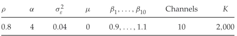
Table 1: True Parameter Setting for Generating the Synthetic Data Set.
ρ α σ2
ε μ β1, . . . , β10 Channels K
0.8 4 0.04 0 0.9, . . . ,1.1 10 2,000
of 1 s. To ensure strong identifiability, we fixedβcandσ2
ε to their true values.
Hence, the inference task is focused on the states and parametersρ,α, and
μ. In addition, each of the three parameters is assigned a flat prior. The implementation details of the four methods are as follows:
r
Single-site Gibbs uses the state transition density proposal for eachstate and random walk proposals for the parameters, in particular, N(θ(i−1),0.012)forρandN(θ(i−1),0.12)for bothαandμ. (For more
details on the conditional distributions, see appendix C in Zammit Mangion et al., 2011.)
r
PMMH uses the same proposals for parameters as the single-siteGibbs sampler. The particles of SMC algorithm are proposed by the state transition density with a population of 1000.
r
HMC uses an identity mass matrix that is further scaled by step sizes. Specifically, in the state sampling stage, we employ 34 integration steps with a step size of 0.03 . For the parameters, 67 integration steps with each step size of 0.015 are chosen. On top of those settings, we also use random integration directions to ensure reversibility.r
RMHMC uses a step size of 0.2 and 25 integration steps for the statesand a step size of 0.8 and 5 integration steps for parameters. Again, a random integration direction is applied at each generalized leapfrog loop.
HMC is tuned in the light of making a trade-off between acceptance rate and number of the leapfrog steps within each Monte Carlo iteration. In other words, we aim to integrate over a certain distance with a small num-ber of integration steps, without rejecting too many proposals. We tuned RMHMC in the same spirit. In addition, simulations show that, RMHMC, benefiting from the use of local geometric structure, with the same number of integration steps, is able to make much larger moves while maintain-ing a high acceptance rate, consistent with the findmaintain-ings in Girolami and Calderhead (2011). Based on this, one can achieve fast mixing with fewer integration steps. With the above settings, as expected, the acceptance rates of HMC and RMHMC shown in Table 2 are much higher than the other two random walk proposal-based methods.
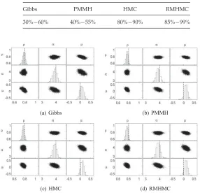
Table 2: Acceptance Rates of All Five Methods.
Gibbs PMMH HMC RMHMC
30%−60% 40%−55% 80%−90% 85%−99%
(a) Gibbs
(c) HMC
(b) PMMH
(d) RMHMC
Figure 1: Full posterior distribution of parameters obtained by four methods, where the true value of each parameter is indicated by a dashed line. There are 20,000 (after 1000 burn-in) posterior samples for each of the three parameters.
hoc shapes within the clouds of samples, implying that the chosen burn-in period is not sufficiently long.
In addition to the posterior profile, by comparing theRˆstatistic from Gelman and Rubin (1992), we further assess each method on the time for convergence to the stationary distribution in Figure 2. This test is carried out by considering five chains with different initializations. Since we have 2004 variables, we show only the statistics for parameters that capture the overall convergence status well. We observe that the Markov chain obtained by a single-site Gibbs sampler is poorly mixed inρ, whereas RMHMC consistently shows the fastest convergence performance.
Figure 2: Logarithm
ˆ
Rstatistics (see Gelman & Rubin, 1992) forρ,α, andμ. Convergence corresponds to an
ˆ
Rvalue close to 1.
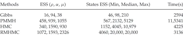
Table 3: ESS and Processing Time Comparison Based on 20,000 Posterior Sam-ples (1000 Burn-In) of States and Parameters Obtained by Single-Site Gibbs, PMMH, HMC, and RMHMC on Synthetic Data Set.
Methods ESS (ρ,α,μ) States ESS (Min, Median, Max) Time(s)
Gibbs 16, 94, 38 46, 98, 210 2594
PMMH 458, 939, 1055 567, 2132, 5129 11,5341 HMC 340, 1590, 930 1152, 4045, 10,979 4225 RMHMC 1072, 1593, 2326 4060, 20,000, 20,000 3136
Note: Each attribute is averaged over 10 runs.
Calderhead (2011) (Liu, 2001, for more details on ESS). In order to make a fair assessment, each method is run 10 times on the same data set and averages tabulated. We note that RMHHC shows the highest ESS scores for both states and parameters and ranks second in processing speed. HMC shows the second-highest ESS score on states, yet the parameter ESS (inρandμ) is similar to PMMH. Further, all methods show significant improvement on ESS when compared to the baseline single-site Gibbs sampler. Finally, results on autocorrelation function (ACF) performance in Figure 3 also lend additional supports to the findings.
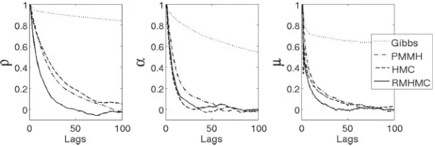
[image:14.432.61.372.288.352.2]Figure 3: The first 100 lags of autocorrelation values of different MCMC meth-ods for each parameter. RMHMC outperforms other methmeth-ods in ρ and μ, whereas inα, HMC drops faster than others, indicating that a unit tensor in
αmay be appropriate.
with real applications, in which the length of data records may be substan-tial in comparison to the synthetic data we have used.
6.2 Modeling Taste Response. This section is a study of the perfor-mance of RMHMC on a rat spike train data set in which the firing pattern of a single cell has been measured under different taste stimuli. The details of the experiment can be found in Di Lorenzo and Victor (2003). Briefly, four taste stimuli are considered: NaCl, sucrose, quinine HCl, and HCl, inducing salty, sweet, sour, and bitter tastes. Under each stimulus, recording trials are separated by a 20 s rinsing and a 1.5 min wait, and each trial consists of a 10 s baseline period with no stimulus, 5 s presentation of stimulus, and 5 s wait.
Recently Zammit Mangion et al. (2011) examined this data set with the SSPP model with an online VB inference framework and showed the ability to detect sudden changes on the model parameters in response to changes in stimuli. The preprocessing steps follow Zammit Mangion et al. (2011), where the 10 s baseline period is considered in the analysis and trials associ-ated with each tastant are concatenassoci-ated to form one contiguous spike train. Due to the response latency and a linear increase on firing rate for the first 250 ms after each stimulus in the data set, which is noted in both Di Lorenzo and Victor (2003) and Zammit Mangion et al. (2011), a temporal rectangular window of 250 ms is applied at the beginning of each 10 s segment. The time resolution is set to 10 ms, which resulted in a small number of bins containing more than one spike. This was adjusted by moving the spike to the nearest empty bin forward in time. The resulting data contained 23,000 time points in cell 9 and 16,000 time points in cells 4 and 11.
Figure 4: Posterior distributions ofαandμgiven the observed spike trains in cells 4, 9, and 11. The parameter space shows good separation of the four tastes.
dynamically separate the firing rate into two major contributors: back-ground noise and underlying neural dynamics, which is driven by the external stimulus. Such a separation makes classification easier when the firing rate in itself cannot discriminate between the tastants. Therefore, the inference we target is the posterior distributions ofα,μ, and the underlying states, given the observed spike train, with the other parameters fixed at :
ρ=0.97,σ2
ε =0.05, andβ=0.5. Figure 4 shows results of this, and it can
be seen that the separation we aimed for is convincingly achieved by the model.
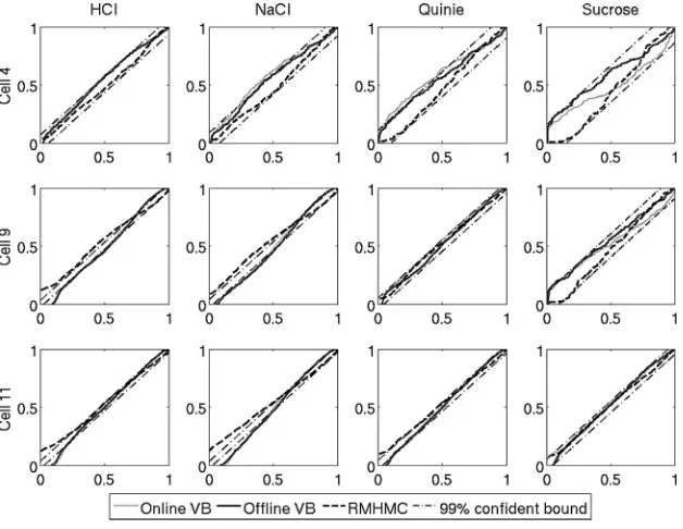
We also assess the model goodness of fit in Figures 5 and 6 using the time-rescaled theorem-based KS test (for details, see Brown, Barbieri, Ventura, Kass, & Frank, 2001) and find that while RMHMC obtained a slightly better fit in cell 4, the results are similar to VB in cells 9 and 11.
Figure 5: Q-Q plot based on time rescaling theorem (Brown et al., 2001) of inferred model by RMHMC, offline VB, and online VB. Thex-axis shows the quantiles, and they-axis shows an empirical cumulative rate function. Ninety-nine percent confident intervals are indicated by the dashed line in each figure. A 45 degree line indicates a perfect match.
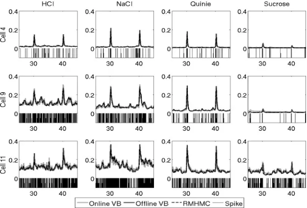
[image:17.432.95.337.387.544.2]Figure 7: A 20 s segment expected spiking probability with respect to state and parameter posteriors obtain by RMHMC, offline VB, and online VB (graphs overlap because the differences among the methods are small). For each panel, thex-axis denotes time with unit in seconds, and they-axis denotes the expected spiking probability measure. The observed spike train is also shown in black bars.
the uncertainty. VB methods, on the other hand, often underestimate the uncertainty within the state transition process due to the independent as-sumption of the mean field approximation (Turner & Sahani, 2010). Note that the number of data points is large in this data set, and given the fact that the posteriors are unimodal, it is reasonable to expect MCMC and VB to show similar performance.
The next section shows results from a different data set in which the data record is much shorter in time and spiking is sparse.
6.3 Parvocellular Neuron Data Set. We now consider another data set from Victor et al. (2007), where the response variability of marmoset parvo-cellular neurons under drifting sinusoidal luminance gratings stimulus is considered. Single cell spiking activities are recorded, where the luminance modulation (LUM) stimuli are presented at 10 different ascending contrast levels.1Each contrast is repeated 13 times within a 3.5 s period for three
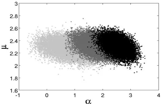
Figure 8: Jointα andμ posteriors. Clusters from right to left correspond to contrast values of 1, 0.5 and 0.35.
trials. We treat the three trials as three parallel channels of spike trains driven by the same stimulus. The time resolution is set to 0.002 s, which guarantees one spike per time bin and yields 1750 time points for each channel.
Similar to the previous example, we use RMHMC to target the posterior distributions ofα,μ, and hidden states given observed spike trains. We fix
ρ=0.8,σ2
ε =0.05, andβ=1 for each channel.
As shown in Figure 8, the resulting posteriors overlap heavily and there-fore are not easy to distinguish between trials with different stimulus types. However, the inferred model is still able to characterize the data quite well according to the KS test results, as shown in Figures 9 and 10. In this case, there are significantly fewer data than in the taste response data set con-sidered previously. RMHMC consistently outperforms both EM and VB in terms of the model goodness of fit across each of the 10 contrast levels. Finally, the expected spiking probabilities are consistent with the data (see Figure 11).
7 Discussion
Figure 10: The mean squared maximum KS distance of each contrast level. Contrast levels 1 to 10 denote 0.0156 to 1 in the data set. Each block of vertical bars corresponds to EM, offline VB, and RMHMC from left to right.
Figure 11: Expected spiking probability with respect to state and parameter posteriors obtained by RMHMC, EM, and offline VB. The left panel and right panels correspond to contrasts of 0 and 1.
[image:21.432.60.372.315.480.2]particular, the metric tensor takes the form of an expected Fisher informa-tion matrix, which is analytically available. Moreover, due to the previously noted unimodality property (Yuan & Niranjan, 2010) of the SSPP model, such a metric tensor is guaranteed to be positive definite, which justifies the suitability of using RMHMC.
In addition to the synthetic example, we compared the performance of the RMHMC with variational Bayes (VB) on a rat taste stimuli data set and monkey parvocellular neuron data set. Results on these experi-ments suggest that the advantage gained using RMHMC is pronounced on short-duration data sets with small numbers of observed spikes. This may be of interest in analyzing nonstationary data using short windows in time. For long time series, VB methods seem preferable, since they offer an at-tractive balance between computational cost and estimation accuracy. How-ever, one should note that the SSPP model may be customized for different modeling tasks. Different choices for the conditional intensity function may lead to VB being intractable. MCMC methods, on the other hand, have the flexibility of adapting to such complex scenarios.
Relating the framework described in this letter, another popular model for characterizing neural spike trains is the point process generalized linear model (Truccolo, Eden, Fellows, Donoghue, & Brown, 2005; Okatan, Wilson, & Brown, 2005), in which the stimuli are treated as canonical parameters in a likelihood model similar to the one considered in SSPP. For inference on this model, Paninski (2004) provides a maximum likelihood formulation, whereas for the Bayesian perspective, both the MCMC and VB approaches have recently been studied and shown good results on decoding the spike trains (Ahmadian, Pillow, & Paninski, 2011; Chen, Kloosterman, Wilson, & Brown, 2010). The SSPP differs from such a paradigm by assuming a latent dynamic process that takes the stimuli as input sources, resulting in a physiologically plausible parameterization. Its inference frameworks including EM (Smith & Brown, 2003), VB (Zammit Mangion et al., 2011), and MCMC discussed in this work, also show good performance on decoding the spike train, while the inferred parameters may serve as discriminant attributes of different physiological states.
For spike train classification, Salimpour, Soltanian-Zadeh, Salehi, Emadi, and Abouzari (2011) show an interesting approach of using the likelihood based on filtered estimates as a discriminator for spike trains responding to various stimuli. Their model treats parameters of the CIF as states in de-riving an extended Kalman filter estimator. This differs from the model we considered, which has a separate underlying dynamical state process. Al-gorithmically, Salimpour et al.’s (2011) work has similarities to the Laplace approximation-based adaptive filters (Smith & Brown, 2003; Eden, Frank, Barbieri, Solo, & Brown, 2004; Koyama, Castellanos P´erez-Bolde, Shalizi, & Kass, 2010).
Table 4: General Computational Cost Comparison.
Gibbs PMMH HMC RMHMC
O((K+1)M) O(NKM) O((L1K+L2)M) O((L1∗K+L∗2)M)
filtering density. Together with other nonlinear filtering methods like un-scented Kalman filter (UKF) (Julier & Uhlmann, 1997; Wan & Van Der Merwe, 2000), they have the potential for constructing efficient propos-als for state updating in PMMH. Such an idea has been explored in the context of SMC (Erg ¨un et al., 2007; Wang et al., 2009). Further, these filter-ing methods can be used to obtain Laplace approximation and variational lower bound of the marginal likelihood, resulting in approximate sampling methods.
As another future extension, instead of the random walk proposals, it is possible to use gradient-based proposals to improve the acceptance rate in PMMH, for example, the Metropolis adjusted Langevin algorithm (MALA), manifold MALA method (Girolami & Calderhead, 2011), HMC, and RMHMC. Despite the severe computational overheads, these ideas are algorithmically attractive, since they offer highly efficient proposal mecha-nisms to tackle problems with high correlations between states and param-eters. We are currently pursuing these avenues.
Appendix: Computation Complexity
Here we give estimates of the orders of computational complexities of the different sampling algorithms used. LetKandMbe the time points and the number of Monte Carlo iterations, respectively.Ndenotes the number of particles used in PMMH.L1andL2are the number of leapfrog steps for states and parameters in HMC. The superscript∗indicates that the number of leapfrog steps in RMHMC is different from those in HMC. In addition, we assume the cost of each parameter updating and other inner calculations to be 1. With these notations, Table 4 shows the estimated complexities.
Acknowledgments
References
Ahmadian, Y., Pillow, J. W., & Paninski, L. (2011). Efficient Markov chain Monte Carlo methods for decoding neural spike trains.Neural Computation,23(1), 46–96. Amari, S., & Nagaoka, H. (2000).Methods of information geometry. New York: Oxford
University Press.
Andrieu, C., Doucet, A., & Holenstein, R. (2010). Particle Markov chain Monte Carlo methods (with discussion).Journal of the Royal Statistical Society: Series B,72, 269– 342.
Brown, E. N., Barbieri, R., Eden, U. T., & Frank, L. M. (2002). Likelihood methods for neural data analysis. In J. Feng (Ed.),Computational neuroscience: A Comprehensive approach(pp. 253–286). London: CRC.
Brown, E. N., Barbieri, R., Ventura, V., Kass, R. E., & Frank, L. M. (2001). The time-rescaling theorem and its application to neural spike train data analysis.Neural Computation,14(14), 325–346.
Carter, C. K., & Kohn, R. (1994). On Gibbs sampling for state space models.Biometrika,
81(3), 541–553.
Chen, Z., Kloosterman, F., Wilson, M. A., & Brown, E. N. (2010). Variational Bayesian inference for point process generalized linear models in neural spike trains anal-ysis. InProceedings of the 2010 IEEE International Conference on Acoustics Speech and Signal Processing (ICASSP)(pp. 2086–2089). Piscataway, NJ: IEEE.
Daley, D., & Vere-Jones, D. (2003).An introduction to the theory of point process(2nd ed.). New York: Springer-Verlag.
Di Lorenzo, P., & Victor, J. (2003). Taste response variability and temporal coding in the nucleus of the solitary tract of the rat.Journal of Neurophysiology,90, 1418– 1431.
Doucet, A., de Freitas, N., & Gordon, N. (2001).Sequential Monte Carlo methods in practice. New York: Springer-Verlag.
Duane, S., Kennedy, A. D., Pendleton, B. J., & Roweth, D. (1987). Hybrid Monte Carlo.Physics Letters B,195(2), 216–222.
Eden, U. T., Frank, L. M., Barbieri, R., Solo, V., & Brown, E. N. (2004). Dynamic anal-ysis of neural encoding by point process adaptive filtering.Neural Computation,
16(5), 971–998.
Erg ¨un, A., Barbieri, R., Eden, U. T., Wilson, M. A., & Brown, E. N. (2007). Construction of point process adaptive filter algorithms for neural systems using sequential Monte Carlo methods.IEEE Transactions on Biomedical Engineering,54(3), 419–428. Fearnhead, P. (2010). MCMC for state space models. In S. Brooks, A. Gelman, G. Jones, & X.-L. Meng (Eds.),Handbook of Markov chain Monte Carlo. Boca Raton, FL: CRC.
Gelman, A., & Rubin, D. B. (1992). Inference from iterative simulation using multiple sequences (with discussion).Statistical Science,7(4), 457–472.
Geweke, J., & Tanizaki, H. (2001). Bayesian estimation of state-space models using the Metropolis-Hasting algorithm within Gibbs sampling.Computational Statistics and Data Analysis,37(2), 151–170.
Girolami, M., & Calderhead, B. (2011). Riemann manifold Langevin and Hamiltonian Monte Carlo methods (with discussion).Journal of the Royal Statistical Society: Series B (Statistical Methodology),73, 123–214.
Ivanov, P., Rosenblum, M., Peng, C., Mietus, J., Havlin, S., Stanley, H., et al. (1996). Scaling behaviour of heartbeat intervals obtained by wavelet-based time-series analysis.Nature,383, 323–327.
Jolivet, R., Kobayashi, R., Rauch, A., Naud, R., Shinomoto, S., & Gerstner, W. (2008). A benchmark test for a quantitative assessment of simple neuron models.Journal of Neuroscience Methods,169, 417–424.
Julier, S., & Uhlmann, J. (1997). A new extension of the Kalman filter to nonlinear sys-tems. InProceedings of the Int. Symp. Aerospace/Defense Sensing, Simul. and Controls
(vol. 3, p. 26). Bellingham, WA: SPIE.
Kass, R. E. (1989). The geometry of asymptotic inference.Statistical Science,4, 188– 234.
Koyama, S., Castellanos P´erez-Bolde, L., Shalizi, C. R., & Kass, R. E. (2010). Approxi-mate methods for state-space models.Journal of the American Statistical Association,
105(489), 170–180.
Liu, J. S. (2001).Monte Carlo strategies in scientific computing. New York: Springer-Verlag.
Neal, R. M. (1993). Probabilistic inference using Markov chain Monte Carlo methods
(Techn. Rep. No. CRG-TR-93-1). Toronto: University of Toronto.
Neal, R. M. (2010). MCMC using Hamiltonian dynamics. In S. Brooks, A. Gelman, G. Jones, & X.-L. Meng (Eds.),Handbook of Markov chain Monte Carlo. Boca Raton, FL: CRC.
Okatan, M., Wilson, M. A., & Brown, E. N. (2005). Analyzing functional connectivity using a network likelihood model of ensemble neural spiking activity.Neural Computation,17(9), 1927–1961.
Paninski, L. (2004). Maximum likelihood estimation of cascade point-process neural encoding models.Network: Computation in Neural Systems,15(4), 243–262. Pitt, M., & Shephard, N. (1999). Filtering via simulation: Auxiliary particle filters.
Journal of the American Statistical Association,94, 590–599.
Rao, C. R. (1945). Information & accuracy attainable in the estimation of statistical parameters.Bull. Calc. Math. Soc.,37, 81–91.
Salimpour, Y., Soltanian-Zadeh, H., Salehi, S., Emadi, N., & Abouzari, M. (2011). Neuronal spike train analysis in likelihood space.PLoS ONE,6(6), e21256. Scott, S. L. (2002). Bayesian methods for hidden Markov models: Recursive
com-puting in the 21st century.Journal of the American Statistical Association,97(457), 337–351.
Shephard, N., & Pitt, M. K. (1997). Likelihood analysis of non-gaussian measurement time series.Biometrika,84(3), 653–667.
Smith, A. C., & Brown, E. N. (2003). Estimating a state-space model from point process observations.Neural Computation,15(5), 965–991.
Turner, R., & Sahani, M. (2010). Two problems with variational expectation maximi-sation for time-series models. In D. Barber, A.-T. Cemgil, & S. Chiappa (Eds.),
Inference and learning in dynamic models. Cambridge: Cambridge University Press. Victor, J., Blessing, E., Forte, J., Buz´as, P., & Martin, P. (2007). Response variability of
marmoset parvocellular neurons.Journal of Physiology,579(1), 29–51.
Wan, E., & Van Der Merwe, R. (2000). The unscented Kalman filter for nonlinear esti-mation. InProceedings of the Adaptive Systems for Signal Processing, Communications, and Control Symposium 2000(pp. 153–158). Piscataway, NJ: IEEE.
Wang, Y., Paiva, A.R.C., Pr´ıncipe, J. C., & Sanchez, J. C. (2009). Sequential Monte Carlo point-process estimation of kinematics from neural spiking activity for brain-machine interfaces.Neural Computation,21(10), 2894–2930.
Yuan, K., & Niranjan, M. (2010). Estimating a state-space model from point process observations: A note on convergence.Neural Computation,22(8), 1993–2001. Zammit Mangion, A., Yuan, K., Kadirkamanathan, V., Niranjan, M., & Sanguinetti,
G. (2011). Online variational inference for state-space models with point process observations.Neural Computation,23(8), 1967–1999.