http://go.warwick.ac.uk/lib-publications
Original citation:
Rousakis, Michael (2012). Expectations and fluctuations : the role of monetary policy. Coventry: Department of Economics, University of Warwick. (The Warwick Economics Research Paper Series (TWERPS) no.984).
Permanent WRAP url:
http://wrap.warwick.ac.uk/45596 Copyright and reuse:
The Warwick Research Archive Portal (WRAP) makes the work of researchers of the University of Warwick available open access under the following conditions. Copyright © and all moral rights to the version of the paper presented here belong to the individual author(s) and/or other copyright owners. To the extent reasonable and practicable the material made available in WRAP has been checked for eligibility before being made available.
Copies of full items can be used for personal research or study, educational, or not-for-profit purposes without prior permission or charge. Provided that the authors, title and full bibliographic details are credited, a hyperlink and/or URL is given for the original metadata page and the content is not changed in any way.
A note on versions:
The version presented here is a working paper or pre-print that may be later published elsewhere. If a published version is known of, the above WRAP url will contain details on finding it.
Expectations and Fluctuations : The Role of Monetary Policy
Michael Rousakis
No 984
WARWICK ECONOMIC RESEARCH PAPERS
Expectations and Fluctuations:
The Role of Monetary Policy
∗Michael Rousakis
University of Warwick
March 23, 2012
Abstract
How does the economy respond to shocks to expectations? This paper addresses this ques-tion within a cashless, monetary economy. A competitive economy features producers and con-sumers/workers with asymmetric information. Only workers observe current productivity and hence they perfectly anticipate prices, whereas all agents observe a noisy signal about long-run productivity. Information asymmetries imply that monetary policy and consumers’ expectations have real effects. Non-fundamental, purely expectational shocks are conventionally thought of as demand shocks. While this remains a possibility, expectational shocks can also have the charac-teristics of supply shocks: if positive, they increase output and employment, and lower inflation. Whether expectational shocks manifest themselves as demand or supply shocks depends on the monetary policy pursued. Forward-looking policies generate multiple equilibria in which the role of consumers’ expectations is arbitrary. Optimal policies restore the complete information equilibrium. They do so by manipulating prices so that producers correctly anticipate their rev-enue despite their uncertainty about current productivity. I design targets for forward-looking interest-rate rules which restore the complete information equilibrium for any policy parameters. Inflation stabilization per se is typically suboptimal as it can at best eliminate uncertainty aris-ing through prices. This offers a motivation for the Dual Mandate of central banks.
JEL Classification: E32, E52, D82, D83, D84
Keywords: Asymmetric information, producer expectations, consumer expectations, business cycles, supply shocks, demand shocks, optimal monetary policy
∗
I am especially grateful to Herakles Polemarchakis for his continuous support and guidance, and his invaluable comments on this paper. I am also indebted to Paulo Santos Monteiro for the many discussions we have had and his advice, and to Michael McMahon and Kostas Mavromatis for their many suggestions. I have also benefited greatly from the comments of Henrique Basso, Pablo Beker, Federico Di Pace, Peter Hammond, Leo Kaas, Guido Lorenzoni, Claudio Michelacci, Juan Pablo Nicolini, Franck Portier, Guillaume Sublet, Juuso V¨alim¨aki as well as of participants in the Warwick Macro Group, the Warwick Lunch Seminars, the XVI Workshop on Dynamic Macroeconomics in Vigo, the 10th Conference on Research in Economic Theory and its Applications in Milos, and the 2011 European Winter Meeting of the Econometric Society in Tel Aviv. Responsibility for the remaining errors is solely mine.
1
Introduction
Recent empirical work suggests that shocks to expectations contribute significantly to economic
fluctuations.1 But how so? This is a recurrent question for academics, practitioners, and op-ed
columnists. There is a growing consensus that if, for instance, consumers overstate the economy’s
fundamentals, the economy booms at the cost of inflation. A recent literature has formalized this
idea:2 non-fundamental, purely expectational shocks behave like demand shocks. When positive,
they increase output and employment, and are inflationary. Stabilizing inflation emerges then as a
natural policy recommendation.3
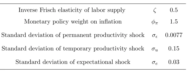
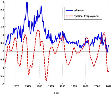
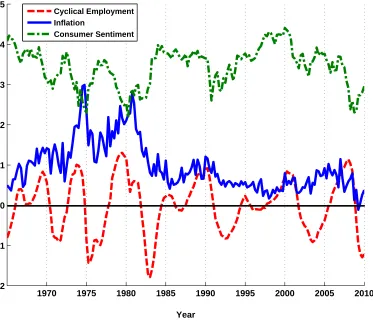
Nevertheless, Figures 1 - 4 show that the US economy was characterized by high cyclical
employ-ment and relatively low inflation in the mid-80s and the second half of the 90s, which are recalled
as periods of exuberant optimism. Notably, Figures 3 and 4 reveal that consumer sentiment and
inflation are negatively correlated.4 An interpretation of expectational shocks as demands shocks
does not seem to fit.
This paper reconsiders the nature of purely expectational shocks within a competitive,
mone-tary, cashless economy where producers and consumers/workers have asymmetric information about
fundamentals and inflation (prices). I show that expectational shocks can have implications for the
business cycle associated with supply shocks: when positive, they increase output and employment,
and they lower inflation, which is incompatible with the Phillips curve.5 Nonetheless, the possibility
that expectational shocks manifest themselves as demand shocks remains. The underlying forces
are producers’ expectations which push toward a supply-shock interpretation and consumers’
expec-tations which push toward a demand-shock interpretation; which one (demand or supply) prevails
depends on the monetary policy pursued.
A natural question that emerges concerns the role of the monetary authority and its optimal
response to shocks. With flexible prices, producers’ incomplete information is the only source of
inefficiency. Asymmetric, as opposed to incomplete but symmetric, information about inflation
(prices) implies that monetary policy has real effects. Optimal policies restore the complete
infor-1
Empirical studies on the contribution of changes in expectations to business cycle fluctuations include Beaudry and Portier (2006), Schmitt-Grohe and Uribe (2008), Blanchard et al. (2009)), Beaudry and Lucke (2010) and Barsky and Sims (2011a,b).
2
See for example Blanchard (2009), Angeletos and La’O (2009), and especially Lorenzoni (2009, 2011).
3
See the baseline case in Lorenzoni (2009).
4
At a quarterly basis (Figure 3), the correlation of consumer sentiment and inflation is−0.53 . Data are described in Appendix B.
5
mation equilibrium. Inflation stabilization per se is typically suboptimal as it at best eliminates
uncertainty arising through inflation without removing producers’ incomplete information.
Opti-mal policies manipulate inflation so that producers correctly anticipate their revenue despite their
uncertainty about productivity. Bearing this in mind, I design targets for forward-looking policies
which restore the complete information equilibrium for any chosen policy parameters.
A competitive (neoclassical) economy features two representative agents, a consumer/worker
and a producer, and a monetary authority. The worker supplies labor to a firm, managed by
the producer, which produces a single commodity. Productivity consists of a permanent and a
temporary component. There is asymmetric information about its current realization: it is specific
and known to the worker, while the producer faces uncertainty about it. The monetary authority sets
the riskless short-term nominal interest rate. I consider two interest-rate rules: a “contemporaneous”
one and a forward-looking one.
Each period is split into two stages: In the first stage, the worker realizes his current productivity
-not its individual components- , both agents observe a noisy public signal about the permanent
(equivalently, long-run) productivity component, and the labor market opens (and closes). In the
second stage, with production predetermined from stage 1 , the commodity and the nominal bond
markets open (and close) and all payments materialize. Prices are flexible in all markets and agents
are price-takers.
The nominal wage, announced in stage 1, reflects the producer’s expectations about productivity
as well as stage 2 inflation (or prices). With constant returns to scale, the scale of production is
pinned down by labor supply. The worker has complete information, so his labor decision and,
consequently, production depend on the nominal wage and the inflation he knows will prevail in
stage 2.
Inflation, in turn, depends on current productivity, on the producer’s expectations about it,
and the consumer’s expectations about long-run productivity in a way decided by monetary policy.
Asymmetric information about current productivity leads agents to form heterogeneous expectations
about the inflation to prevail; this opens the door to monetary policy. Further, to the extent that
inflation depends on the consumer’s expectations about long-run productivity, the producer needs
to second-guess the consumer. Then the consumer’s expectations also have real effects, indirectly,
through inflation. Therefore, that inflation is realized after the labor market has cleared not only
prevents productivity from being revealed, but, in combination with asymmetric information, it
Purely expectational shocks affect both agents’ expectations. The consumer’s expectations
about long-run productivity push toward a demand shock interpretation. A consumption
smooth-ing motive is behind this. Consider, for instance, positive purely expectational shocks. A consumer
overly optimistic about the long-run prospects of the economy raises his current demand. If the
pro-ducer had complete information about current productivity, flexible prices would increase and wages
would proportionally adjust leaving the real wage intact. However, under incomplete information,
the producer overestimates the inflationary pressure caused due to the consumer’s expectations. As
a result, the nominal wage increases more than proportionally and a higher real wage prevails. This
induces the worker to increase his labor supply and production to expand.
The producer’s expectations about current productivity per se point toward a supply shock
in-terpretation. A higher real wage reflects the producer’s overly optimistic expectations; employment
increases, production expands and, for a certain demand level, prices need to fall for the commodity
market to clear.
It should not perhaps come as a surprise that the producer’s incomplete information manifests
itself as a distortion in the labor wedge originating from the labor demand side. The labor wedge is
defined as the ratio of the marginal product of labor to the marginal rate of substitution of leisure
for consumption.6 Chari et al. (2007) find that it is countercyclical and accounts for more than half
of the US output variance. When the real wage exceeds the marginal product of labor, the labor
wedge falls. Positive expectational shocks, then, induce a countercyclical labor wedge.7
Whether expectational shocks cause an inflationary or a deflationary pressure depends on the
monetary policy pursued. Taking into account that employment and output both increase (positive
co-movement), it follows that it is up to the monetary authority whether a demand or a supply
shock interpretation best fits expectational shocks.
In particular, the policy weight on the current output gap is central to which interpretation
prevails. To see this, fix the real interest rate and note that, for a “contemporaneous” rule, expected
inflation is zero, which implies that the real interest rate coincides with the nominal one. The
nominal interest rate targets inflation and the output gap. A positive expectational shock results in
a positive output gap. A higher weight on the output gap implies less inflationary pressure which,
in fact, may turn to a deflationary one.
6
See for example Hall (1997), Chari et al. (2007) and Shimer (2009).
7
Turning to productivity shocks, agents’ expectations underreact in response to positive
produc-tivity shocks. As a result, a lower real wage prevails which induces employment to fall,8 whereas
output increases, however by less than under complete information. Following the same line of
thought as above, the policy weight on current output gap determines whether productivity shocks
are inflationary or disinflationary. Of course, agents learn over time and their expectations
eventu-ally converge to the underlying productivity level.
Considering forward-looking policies, the main difference with “contemporaneous” ones is that
forward-looking policies generate a continuum of equilibria for any choice of policy parameters.9
Importantly, what distinguishes equilibria is the role of the consumer’s expectations which is
ar-bitrarily specified. Furthermore, the short-run volatility of output due to expectational shocks is
considerably higher under forward-looking policies than under “contemporaneous” ones. These
results can contribute to the discussion about the desirability of forward-looking policies.10
The nominal implications for forward-looking rules also differ, even after controlling for the
consumer’s expectations. This is because “contemporaneous” interest-rate rules pin down
infla-tion, whereas forward-looking ones pin down price levels. To see this, consider a positive purely
expectational shock and let prices depend positively on the producer’s expectations, which is true
for “active” policies, i.e. policies in which the monetary authority responds to inflation more than
one-to-one. Price levels exhibit a non-monotonic pattern in response to expectational shocks: they
increase on impact, however as agents update their beliefs over time, they gradually return to
their long-run level. Thus, positive expectational shocks cause an inflationary pressure on impact
and a deflationary one from the following period onwards. By the same logic, positive permanent
productivity shocks are inflationary, until prices reach their higher steady-state level.
The producer’s incomplete information is the only source of inefficiency. Optimal monetary
poli-cies restore then the complete information equilibrium. To do so they manipulate inflation (prices)
so that the producer correctly anticipates his stage-2 revenue, even though still uncertain about
current productivity. Inflation stabilization per se is typically suboptimal as it at best eliminates
8 In the business cycle literature, Gali (1999) and Basu et al. (2006) also argue that positive technology shocks
cause a temporary fall in employment.
9As my focus is on the effects of purely expectational shocks as well as those of productivity shocks, I do not
discuss determinacy in the sense, for example, of Clarida et al. (2000) or Bullard and Mitra (2002) (although that discussion has been recently revived with Cochrane (2011)) . Nevertheless, it is important to mention that there is no real indeterminacy here, since possible “sunspot” shocks lie outside the information sets of both agents thereby having no real effects, a point on which I elaborate below. I resume this discussion in fn. 52 .
10 Clarida et al. (1999, 2000) and Giannoni and Woodford (2003) also consider forward-looking policies, however
the indirect, inflation, channel of expectations without removing the producer’s uncertainty about
current fundamentals. I design forward-looking interest-rate rules which restore the complete
infor-mation equilibrium. The rules “punish” deviations of expected inflation and expected growth from
targets which adjust to their complete information levels.
In an extension, I consider a forward-looking monetary authority with superior information and
let it communicate its information with noise. The noise could be thought of as a measurement error
or a monetary policy shock. The nominal interest rate serves then as an endogenous public signal.
To the extent that prices depend positively on productivity, I show that positive measurement
errors and monetary policy shocks raise the producer’s expectations about the following period’s
productivity which results in higher prices and output.
Related literature. The idea that changes in expectations affect the business cycle has its origins
at least in Pigou (1926) and has recently been revived by Beaudry and Portier (2004).11 Christiano
et al. (2010) show that expectational shocks are disinflationary in a New-Keynesian framework.12
However, this strand of literature distinguishes between shocks to current and future productivity,
whereas I emphasize the distinction between fundamental and non-fundamental shocks to
expecta-tions.
This paper lies in the literature following Phelps (1970) and Lucas (1972) which has formalized
the idea that incomplete information can open the door to non-neutralities of non-fundamental
factors.13 The closest paper is Lorenzoni (2009). Lorenzoni (2009) restricts attention to the
con-sumer side within a New-Keynesian framework and suggests that purely expectational shocks cause
effects associated with demand shocks. Instead, I consider both the producer and the consumer
side in a competitive economy with flexible prices14 and suggest that purely expectational shocks
can behave like supply or demand shocks depending on the monetary policy pursued. To the best
of my knowledge, this paper is the first to suggest so.
This paper shares with Weiss (1980), King (1982) and Lorenzoni (2010) the idea that monetary
11
See also Beaudry and Portier (2006, 2007) and Jaimovich and Rebelo (2009).
12
It has also been suggested in the empirical work of Barsky and Sims (2011b).
13
Polemarchakis and Weiss (1977), Weiss (1980), King (1982), Bulow and Polemarchakis (1983) and, especially, Grossman and Weiss (1982) are related papers of the early literature. The literature has been revived with Woodford (2001), Morris and Shin (2002), Mankiw and Reis (2002) and Sims (2003). Hellwig (2008), Mankiw and Reis (2010), Lorenzoni (2011) and Chapter 9 in Veldkamp (2011) offer excellent surveys of the literature.
14 A strand of literature, which for instance includes Angeletos and La’O (2009), Angeletos and La’O (2011a) and
policy is non-neutral when there is asymmetric information about variables the monetary authority
will respond to.15 Crucially, it is asymmetric, rather than incomplete but symmetric, information
that breaks the policy irrelevance, proposed in Sargent and Wallace (1975, 1976). Furthermore, the
proposed optimal policies here differ from the one in Weiss (1980). In Weiss (1980), prices perfectly
reveal the unknown fundamentals, while here prices are observed with a delay, so, by construction,
this possibility is non-existent.
The structure of the paper is as follows. Sections 2 and 3 present the model. Section 4 considers
a “contemporaneous” interest-rate rule and shows that purely expectational shocks can have the
features of demand or supply shocks for different policy specifications. Section 5 presents and
analyzes the equilibria when a forward-looking interest-rate rule is followed and, in an extension,
endows the monetary authority with superior information. Section 6 discusses the role of monetary
policy and proposes optimal policies. Section 7 concludes.
2
Environment
The competitive economy features two agents: a representative consumer/worker supplying labor
to a representative firm he owns and a producer managing the firm. The firm produces a
non-storable commodity. The economy is cashless and the only relevant financial market is a nominal
bond market; a monetary authority sets the price of a riskless short-term nominal bond according
to a “Taylor-type” rule.16 Agents are price-takers in all markets. Time is discrete and infinite
commencing in period 0. Each period comprises two stages: in stage 1 only the labor market opens,
whereas in stage 2 the commodity and the nominal bond markets open.
The consumer’s preferences are given by
E0c
∞ X
t=0
βtU(Ct, Nt), (1)
with period-tutility
U(Ct, Nt) = logCt −
1 1 +ζ N
1+ζ
t . (2)
Ct and Nt denote consumption and employment in period t, respectively, and ζ > 0 denotes
the inverse of the constant marginal utility of wealth (“Frisch”) elasticity of labor supply. The
consumer’s time preference is parametrized by β ∈(0,1) .
15
Recent papers studying monetary policy in environments with informational frictions include Adam (2007), Paciello and Wiederholt (2011) and Angeletos and La’O (2011b).
The consumer faces a sequence of budget constraints given by
PtCt + QtBt+1 = Bt + WtNt + Πt, (3)
whereQt andBt+1 denote the price and holdings of nominal bonds maturing int+ 1 , respectively,
Pt and Wt the commodity price and the nominal wage in t, respectively, and Πt the firm’s profits
that accrue to the consumer.
The firm’s technology is
Yt = AtNt, (4)
where At denotes the worker’s productivity.
Productivity consists of a permanent and a temporary component (henceforth lowercase letters
will denote natural logarithms),
at = xt + ut, (5)
where x and u denote the permanent and temporary components, respectively. Productivity - not its components - is specific and known to the worker, whereas the producer faces uncertainty about
it.17
The permanent componentxt follows a random walk stochastic process
xt = xt−1 + t, (6)
wheretis an i.i.d shock and∼N(0, σ2) . The temporary componentutis i.i.d. andu∼N(0, σu2) .
All agents have costless access to a public signal about the permanent productivity component
st = xt + et, (7)
where et is i.i.d. ande∼N(0, σ2e) . Shocksu,, and eare mutually independent. Hereafter, I will
callea purely expectational shock.
The distinction between permanent and temporary productivity introduces persistence in the
shock effects.
17
2.1 Timing
Each period is divided into two stages. In stage 1, the consumer realizes his temporal productivity
at, agents and the monetary authority observe the public signalstabout the permanent productivity
component, and the labor market opens (and closes).
Let me note at this point that I split stage 1 into two sub-stages, although I will not make a
distinction between these hereafter: in the first sub-stage of stage 1 , after the new information is
realized, the nominal wage is announced which, due to constant returns to scale, is independent of
the labor submitted. The producer decides whether to “accept” it if it solves his problem, in which
case he commits to accommodate any labor supply, or not. With the equilibrium nominal wage
announced in sub-stage 1 , in sub-stage 2 of stage 1 the worker decides on his labor supply and,
since -as I argue below- he has complete information, his consumption and bond holdings.
In stage 2 , with production predetermined from stage 1 (sub-stage 2) , the commodity and the
nominal-bond markets open (and close). I specify the role of the monetary authority in the following
section. All payments materialize in stage 2 and are perfectly enforceable.
3
Towards Equilibria
The producer’s labor demand in stage 1 maximizes the firm’s expected profits, Etp[λtΠt|It,p1] ,
conditional on the producer’s information set in stage 1, It,p1.18 Taking into account the firm’s technology (4) , period-t profits are given by Πt = (PtAt−Wt)Nt. Profits are evaluated according
to the consumer/owner’s period-t Lagrange multiplier, λt. Constant returns to scale imply that
the producer accommodates any labor supply at the following wage:19
Wt =
Etp[λtPtAt]
Etp[λt]
. (8)
The consumer has complete information about the state of the economy and, as a result, makes
all decisions in stage 1. He chooses consumption, labor supply, and bond holdings to maximize his
expected utility (1) - (2) subject to his sequence of budget constraints (3) and a usual
no-Ponzi-scheme constraint. Nominal bonds are in zero net supply, hence market clearing in the nominal
18Henceforth, the producer’s expectations will always refer to his expectations as of stage 1 unless otherwise stated. 19 It is central in the paper that the nominal wage prevailing in stage 1 be such that the producer’s expected
bond market requires Bt+1 = 0 for all t. As such, I suppress bond holdings from the state of the
economy. The consumer’s optimality conditions are20
Ntζ = Wt
PtCt
(9)
Ct =
Qt
βPt
Etc[Pt+1Ct+1], (10)
where Etc[·] refers to the consumer’s expectations conditional on his information setItc.
3.1 Linear equilibria
I focus on linear equilibria.21 All equilibria are rational expectations equilibria. In log-linear form
the optimality equations are22
wt = Etp[at] + Etp[pt] (11)
ζnt = wt − pt − ct (12)
ct = −logβ+ logQt +Etc[ct+1 + πt+1]. (13)
Combining (11) and (12) results in
ζnt = Etp[at] + Etp[pt] − pt − ct. (14)
I use the optimality conditions (13) and (14) in the rest of the analysis.
The existence of a monetary policy rule can get round the equilibrium indeteterminacy, nominal
or real depending on whether agents have complete information or not, that would have prevailed
in its absence. However, as Section 5 illustrates, the presence of a monetary authority per se need
not be enough.
20
Appendix A.1 provides the equilibrium definition and offers an analytical demonstration of the agents’ problems.
21
I ignore whether non-linear equilibria exist.
22
Monetary authority. The monetary authority sets the gross nominal interest rate (equivalently,
the inverse of the logarithm of the nominal bond price) ,it = −logQt, according to an interest-rate
rule. Two commonly used rules will be considered in sequence, a contemporaneously-looking one
(henceforth, rule 1) and a forward-looking one (henceforth, rule 2) :23
it = − logβ + φππt + φy(yt−at) (Rule 1)
it = −logβ + φπEtm[πt+1]. (Rule 2)
where it denotes the nominal interest rate and πt denotes inflation in period t, defined as πt :=
pt−pt−1. In the case of rule 1, the monetary authority targets the output gap defined as the
deviation of output from its complete information counterpart at. I restrict attention to positive
values of the policy weights, φπ andφy.
The monetary authority’s information is solely based on the sequence of public signals as well as
information extraction from prices and quantities. In Section 5.5, I let it be endowed with superior
information when it follows rule 2 and subsequently study the information extraction problem of
the agents. I consider more rules in Section 6 which explicitly studies the optimal monetary policies
in the current framework.
3.2 Expectations and the state of the economy
The state of the economy as of periodtcoincides with the the entire history Ψt = {(aτ)τt=0,(sτ)tτ=0}.
Past realizations of productivity and the public signal are part of the current state due to the agents’
formation of expectations. In particular, the evolution of the agents’ expectations about
perma-nent productivity is given by the Kalman filter algorithm. This is because inflation (prices) and/or
quantities perfectly reveal productivity in stage 2 of each period. For this reason, the monetary
authority’s information set when it steps in, Itm, coincides with the state. It follows then that
Itm = It,p2 = Itc = Ψt. The producer’s expectation about current productivity as of stage 1
coin-cides with his expectation about its permanent component which follows from (5) and the fact that
his information set in stage 1 , which I show in the next section, isIt,p1 = {(aτ)tτ−=01 ,(sτ)tτ=0}. More 23 Rule 1 has been suggested by Taylor (1993, 1999) to capture adequately the Fed’s policy during the period
analytically and bearing (5) in mind, agents and the monetary authority’s expectations evolve as
Etp[at] = Et,p1[xt] = (1−µ)Etp−1,2[xt−1] + µ st (15)
Et,p2[xt] = Etc[xt] = Etm[xt] = (1−k)Etc−1[xt−1] + k[θ st + (1−θ)at], (16)
whereµ , k , θ depend on the variancesσ2
,σe2,σ2u and are in (0,1) . Appendix A.2 offers an explicit
treatment of the formation of expectations.
4
Equilibrium under Rule 1: Demand or Supply?
4.1 Complete information benchmark
Consider the case in which the state of the economy is common knowledge. Then, the real side of the
economy is determined irrespectively of the public signal and the pursued monetary policy; we can
confirm thatn∗t = 0 andy∗t = at. On the nominal side, conjecture thatπt = ϑ1Etc[xt] +ϑ2atand
then confirm thatπ∗t = φ1
π(E
c
t[xt]−at).The consumer’s expectations about permanent (long-run)
productivity have only nominal effects: a consumption smoothing motive leads to changes in the
consumer’s current demand depending on his expectations about permanent productivity; however,
flexible prices appropriately adjust in stage 2 and the nominal wage proportionally adjusts in stage
1 leaving the real wage intact and preventing the consumer’s expectations from having real effects.
4.2 Incomplete information
Conjecture that
ct = ξ1Etp[at] + ξ2at (C1)
πt = κ1Etp[at] + κ2Etc[xt] + κ3at. (C2)
Conjectures (C1) and (C2) imply the state of the economy can be summarized as Ψt =
{Etp[at], Ect[xt], at}. This is a direct consequence of the way agents form their expectations,
de-scribed in Section 3.2, which disciplines the treatment of public signals and productivities within the
state. The monetary authority can fully extract the current state by observing the public signal in
(respectively, (C1)) perfectly reveals productivityat. In other words, when the monetary authority
steps in at the beginning of stage 2 , it shares the same information set with the consumer. This
applies to the producer in stage 2 as well; that is Itm = It,p2 = Itc = Ψt.
Adding and subtracting pt−1 in the labor market optimality condition (14) and combining the
Euler equation (13) with rule 1 implies
ζnt = Etp[at] + Etp[πt] − πt − ct (17)
ct = −[φππt + φy(yt−at)] + Etc[ct+1 + πt+1], (18)
respectively.
Combining conjectures (C1) and (C2) with the optimality conditions, (17) and (18), and market
clearing (Appendix A.3 collects the derivations) yields
yt = ξ1Ept[at] + (1−ξ1)at (19)
πt =
1
φπ
[−(1 +φy)ξ1 Etp[at] + Ect[xt] + [(1 +φy)ξ1−1]at] (20)
ξ1 =
φπ − 1 + k(1−θ)
φπ(1 +ζ) − (1 +φy)
, (21)
wherek,θare parameters associated with the consumer’s learning problem introduced previously and derived in Appendix A.2 .24
Equation (19) shows that output is a weighted average25 of productivity and the producer’s
expectations about it. The respective weights depend on the Frisch elasticity of labor supply,
parametrized by ζ, and the monetary policy parametersφπ,φy.
The presence ofφπ, φy in (19) leads to the first key remark: monetary policy is non-neutral.
This is attributed to theheterogeneityof the agents’ expectations in stage 1 about inflation in stage
2 as we can see from (17) . Of course, heterogenous expectations are attributed to the agents’
asym-metric information about current productivity. Crucially, incomplete yet symasym-metric information
would imply a neutral monetary policy.
24 Output is non-stationary. Stationarity can be restored by normalizing it with the permanent productivity
component. For instance, in the case of output we could instead useYts = eYxtt (yts = yt −xt in logs) . However,
throughout the paper I use the non-normalized variables.
A second key remark is that the consumer’s expectations have real effects despite prices being
flexible. Once again, this is a direct consequence of asymmetric information. To the extent that
inflation depends on the consumer’s expectations, the producer needs to second-guess the consumer
when forming expectations about inflation.26 In particular, as (90) in Appendix A.3 shows,
Etp[Etc[xt] ] = Etc[xt] + k(1−θ) (Etp[at] − at).
What matters for the labor decision and hence production -through the inflation channel- is the
wedge between the producer’s and the consumer’s expectations about inflation. Given conjecture
(C2) and the fact that Etc[πt] = πt, it follows that
Etp[πt] − Etc[πt] = Etp[πt] − πt = [κ2k(1−θ) + κ3] (Etp[at]− at). (22)
The presence of the parameterκ2 in (22) attests that the consumer’s expectations have real effects.
Importantly, what lies in the common information of the agents (for example, the producer’s
expectations) and what lies outside both agents’ information sets (possibly, non-fundamental shocks
- see fn. 52) has no real effects through the inflation channel.
I will first discuss purely expectational shocks, which operate only through agents’ expectations.
Insulating the analysis from productivity shocks will allow me to focus solely on the “mechanics” of
agents’ expectations. Subsequently I discuss productivity shocks which operate both directly and
through agents’ expectations. Before continuing, let me point out that
κ1 + κ2 + κ3 = 0 (23)
κ1 + κ3 = −
1
φπ
. (24)
Combining (23) and (24) implies κ2 = φ1π > 0 , which we can see in (20) ; the consumer’s
expectations are positively related to inflation, and, consequently, indirectly through inflation
pos-itively related to output. The logic underlying this is a permanent income hypothesis one: if, for
instance, a purely expectational shock leads the consumer to overstate the long-run prospects of
the economy, consumption smoothing results in an increase in current demand which in turn causes
an inflationary pressure. If the producer had complete information, prices would fully absorb the
26
increased demand in stage 2 and nominal wages would proportionally adjust in stage 1; both would
imply an unaffected real wage and, as a result, the absence of real effects. However, this is not
the case under incomplete information: an overly optimistic producer -the public signal coordinates
agents- overestimates the inflationary pressure. This implies the nominal wage increases more than
proportionally compared to inflation, which results in a higher real wage. The latter causes
la-bor to increase and production to expand, therefore partly accommodating the increased demand.
Purely expectational shocks via the consumer’s expectations push then toward a demand shock
interpretation.
Turning to the producer, we can see from (19) - (21) that his expectations cause output and
inflation to move in opposite directions. In other words, they point toward a supply-shock
interpre-tation.27 A sufficient condition for the producer’s expectations to be positively related to output
and negatively related to inflation is φπ > max{1+1+φζy,1}.28 That is for sufficiently “active”
poli-cies, expectational shocks via the producer’s expectations push toward a co-monotone supply shock
interpretation. As I have already implied, the inefficiency caused due to the producer’s incomplete
information manifests itself as a distortion in the labor optimality condition. In particular, it causes
a shift in labor demand: the overly optimistic, for instance, expectations of the producer will result
in a higher real wage. This induces the worker to increase his labor supply and, as a result,
pro-duction to expand. For a given demand level, this causes a deflationary pressure; prices need to fall
for the commodity market to clear.
Will a demand or a supply shock interpretation prevail for purely expectational shocks?
Suppose that the expectational shock affects the agents’ expectations in the same way.29 Then
it follows that a positive expectational shock lowers inflation as long asκ1 +κ2 < 0 . By (23) and
(24) , this is equivalent to requiring κ3 > 0 . Inspecting (20), we can see that the term κ2 does
not respond to changes in the monetary policy weight on the output gap,φy, whereas κ3 increases 27
As already argued, since the producer second-guesses the consumer when forming expectations about inflation, the consumer’s expectations matter indirectly as the termκ2k(1−θ) in (22) shows. In fact, sinceκ2 > 0 , this term
only accentuates the supply shock interpretation as (92) in Appendix A.3 shows.
28 For min{1+φy
1+ζ ,1−k(1−θ)} < φπ < max{
1+φy
1+ζ ,1 −k(1−θ)}, positive expectational shocks behave like
negative supply shocks: they lower output and raise inflation. For appropriate policy parameters (φπ, φy) , inflation
depends negatively on productivity. Then the indirect, inflation, channel of expectations lowers the total effect of the producer’s expectations: an overly optimistic producer expects the worker to be more productive than he is, while inflation lower than it will actually be. For the suggested parameter values, the negative indirect effect outweighs the positive direct one. As a result, the nominal wage increases by less than inflation, hence, the real wage falls compared to its complete information counterpart, which induces the worker to decrease his labor supply.
29 That is I assumek θ = µin the learning problems of the agents. This is a good approximation if the temporary
in it;30 the sign of κ3 depends on how the policy weight on the output gap relates to the Frisch
elasticity of labor supply 1/ζ. In particular, a value of φy greater than or equal to the inverse
Frisch elasticity of labor supply ζ is a sufficient condition for κ3 to be positive and, consequently,
expectational shocks to be negatively related to inflation.31
The picture that emerges is that expectational shocks can exhibit features associated with supply
or demand shocks depending on the monetary policy pursued. The policy weight on the current
output gap is central to how expectational shocks manifest themselves. In particular, as long asφπ >
max{1+φy
1+ζ ,1}, a higher weight on the output gap pushes toward a supply shock interpretation.
To provide an intuition for this, first note that (20) implies expected inflation is zero, that is the
nominal and the real interest rate coincide:
rt = it = φππt + φy(yt − at). (25)
Fix for a moment the real interest rate and consider the case of overly optimistic expectations
which implies a positive output gap. Controlling for general equilibrium effects, the higher the
policy weight on the output gap, the lower the inflationary pressure has to be for the real rate to
remain constant.32
However, the real -and, hence, the nominal- interest rate increases in response to a positive
purely expectational shock. This is a consequence of the overreaction of expectations: expected
future output increases by more than current output since the latter is in part disciplined by current
productivity, whose long-run component agents overstate. To what extent or whether this increase
will be translated into higher inflation depends on the weight put on the (positive) output gap.
Turning to productivity shocks, φπ > (1 +φy) max{1+1ζ, kζ(1−−φyθ)} is a sufficient condition for
them to be positively related to output. On the nominal side, maintaining the assumption that
ex-pectational shocks affect the agents’ expectations in the same way, a direct implication of (23) and
(24) is that productivity and expectational shocks cannot both increase or lower inflation. To
con-nect the results with the previous analysis, consider a positive productivity shock. Under complete
information, inflation would depend positively on the wedge between the consumer’s expectations
and productivity. Following a positive productivity shock the consumer’s expectations underreact;
as a result, demand underreacts as well which implies that prices must fall for the market to clear.
30A sufficient condition for this is thatφ
π > 1 .
31The termκ
3exhibits discontinuity at φπ(1 +ζ) −1 . As a result, this is true as long asφy < φπ(1 +ζ)−1 .
32
One may wonder what happens when the policy weight on inflation, φπ, changes. In fact, general equilibrium
effects complicate things considerably as both κ2 and κ3 (alternatively, κ1) depend on φπ. As a result, a similar
However, under incomplete information, prices will not fall as much as they would under complete
information, whereas they can even increase. The reason is that the producer’s expectations also
underreact, hence supply underreacts as well.
Along the lines of the above analysis, the weight on the output gap proves to be key as to how
supply responds. Revisiting the real side, the underreaction of the producer’s expectations implies
that the increase in output falls short of the increase in productivity, therefore the output gap is
negative and employment falls. Holding the real and, since they coincide, the nominal interest rate
constant, the higher the weight on the output gap, the lower the nominal interest rate will be, hence
the less the required fall in prices (see also (25)) . However, both the nominal and the real interest
rate fall after a positive productivity shock, a consequence of the underreaction of expectations.
Last, note that forEtp[at] = atthe complete information equilibrium prevails.
4.3 Labor wedge
Formalizing the intuition above, the producer’s incomplete information has an impact on his labor
demand and, consequently, distorts the labor optimality condition. This causes fluctuations in the
labor wedge. Following Chari et al. (2007) and Shimer (2009), the labor wedge is defined as the
ratio of the marginal product of labor to the marginal rate of substitution of leisure for consumption
by construction equal to 1−1τ
n,t in the expression below:
−Un,t
Uc,t
= (1−τn,t)M Pn,t.
Un,tand Uc,t denote the marginal disutility of labor and marginal utility of consumption,
respec-tively, andM Pn,tdenotes the marginal product of labor in periodt. The above expression becomes
in this case
Nt−(1+ζ) = 1 1−τn,t
.
Under complete information, Nt∗ = 1 and the labor wedge is equal to 1 . Under incomplete information this will generally not be the case; switching to logs and using nt = yt − at from the
firm’s technology implies
nt =
φπ − 1 + k(1−θ)
φπ(1 +ζ) − (1 +φy)
(Etp[at] − at) . (26)
Forφπ > max{1+1+φζy,1}, employment depends positively on the distance of the producer’s
expec-tations from the underlying productivity. The labor wedge in logs is given by the LHS below:
−log (1−τn,t) = −
[φπ − 1 + k(1−θ)] (1 +ζ)
φπ(1 +ζ) − (1 +φy)
Maintaining that φπ > max{1+1+φζy ,1}, in caseEtp[at] > at, the log-labor wedge is negative, and
positive, otherwise. Then purely expectational shocks induce a countercyclical labor wedge. This
is easy to see: a positive, for instance, purely expectational shock raises output whereas it lowers
the labor wedge. This is in line with the documented countercyclicality of the labor wedge (see
for example Chari et al. (2007) and Shimer (2009)) and suggests that purely expectational shocks
can possibly account for it. Interestingly, fluctuations in the labor wedge depend on the monetary
policy pursued. Section 6 elaborates on this.
4.4 Equilibrium dynamics
I deal with this case numerically, even though a closed-form representation of the dynamics can be
obtained along the lines of Section 5.3.4 below. The baseline parametrization is in Table 1. In that
I follow Lorenzoni (2009) and one may check the references therein. The parametrization implies
the Kalman gain terms, µ and k, are 0.22 and 0.23 , respectively, whereas the relative weight the consumer places on the public signal, θ, is 0.96 . In addition, I initially set the response to the output gap φy = 0.5 .33
Before continuing with the impulse response functions, let me point out that the stochastic
steady state is pinned down by the permanent productivity component xt, which by (6) evolves as
a random walk (see also fn. 24). The steady state is typically different from the efficient, complete
information level of the economy which is pinned down by aggregate productivityat. In the analysis
of the impulse response functions below, the economy has already reached its steady-state which,
I assume, coincides with its complete information counterpart before any shocks hit. As such, the
two will remain coincidental after a permanent productivity or an expectational shock and they
will only differ on impact following a temporary productivity shock. In particular, the steady state
is given by a = x and Ep[a] = Ec[x] = x. With no loss of generality, I set x = 0.34 In all figures, impulse response functions are for one standard deviation shocks. Periods, appearing on
the horizontal axis of the figures, are interpreted as quarters.
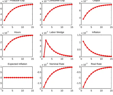
Figure 5 shows the impulse responses to positive purely expectational shocks. As already argued,
as expectations increase, output and employment increase, the labor wedge falls and the interest
rates increase. For the considered parametrization, inflation falls. With no change in the underlying
productivity, all effects die out in the long run and variables return to their steady-state values.
33The monetary policy parameters are based on Taylor (1993) .
34 These implyy = x,n = 0,π = 0, andr = i = −logβ. For ease of exposition, I have suppressed constants,
Table 1: Calibrated parameters
Inverse Frisch elasticity of labor supply ζ 0.5 Monetary policy weight on inflation φπ 1.5
Standard deviation of permanent productivity shock σ 0.0077
Standard deviation of temporary productivity shock σu 0.15
Standard deviation of expectational shock σe 0.03
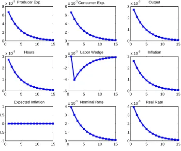
Figure 6 shows that after a positive permanent productivity shock agents expectations
underre-act. This causes an increase in output, however by less than under complete information, which in
turn causes a fall in employment. As employment falls, the labor wedge increases and is therefore
procyclical. For the considered parametrization, inflation increases, whereas, since expectations
underreact, the nominal and the real interest rate fall. As expectations converge to the underlying
higher productivity level, all variables converge to their steady-state levels.
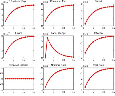
The impulse responses to a temporary productivity shock (Figure 7) are initially similar to the
ones of a permanent productivity shock and, subsequently, to the ones of an expectational shock.
As argued above, this is because they affect productivity only on impact, whereas from the following
period onwards they serve as purely expectational shocks.
As I have already pointed out, the impulse responses when rule 1 is followed are generally
sensitive to the specification of the monetary policy rule and, in particular, to the policy weight on
the output gap, φy. Consider the case in which the authority does not respond to the output gap,
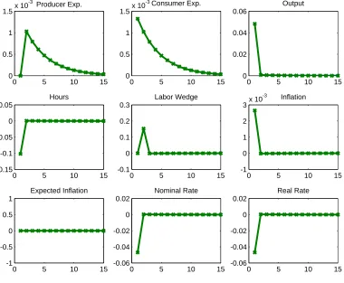
that isφy = 0 , with all other parameters as in Table 1 . Figures 8 - 10 show the impulse responses to
one standard-deviation positive permanent productivity, expectational, and temporary productivity
shocks, respectively. While everything else remains unchanged, the implications for inflation are
reversed. In particular, positive permanent productivity shocks lower inflation whereas positive
expectational shocks increase inflation. The last results are in line with Lorenzoni (2009). Notably,
unlike in Lorenzoni (2009), they are generated in a perfectly competitive environment where prices
are flexible and the real interest rate can freely adjust.
Juxtaposing figures 5 and 8 illustrates the first main result of the paper: purely expectational
shocks can behave like supply or demand shocks. A natural question is why the current framework
ex-pectations and, second, the presence of asymmetric information between consumers and producers.
Crucially, the latter pushes monetary policy and the consumer’s expectations through the door.35
The producer’s expectations point toward a supply-shock interpretation, whereas the consumer’s
expectations, as in Lorenzoni (2009), point toward a demand-shock interpretation. The monetary
authority decides which one will prevail.
5
Equilibria under Rule 2: Beyond Demand and Supply
5.1 Complete information benchmark
Like before, under incomplete information yt∗ = at and n∗t = 0. Conjecture for prices that pt =
ϑ3Etc[xt] + ϑ4at. The Euler equation (13) becomes
Ect[at+1]− at = (φπ−1) (Etc[pt+1] − pt). (28)
A family of solutions is given by p∗t = φ1
π−1at + ϑ3E
c
t[xt] ; price levels depend arbitrarily on the
consumer’s expectations.
5.2 Incomplete information
Consider the conjectures:36
ct = ξ3Etp[at] + ξ4at (C3)
pt = κ4Etp[at] + κ5Etc[xt] + κ6at. (C4)
Conjectures (C3) and (C4) imply the state can sufficiently be described by Ψt = {Etp[at], Etc[xt], at}.
The information sets of the agents and the monetary authority are like before. SinceItm = Itc, the Euler equation (13) becomes
Etc[ct+1]− ct = (φπ−1) (Etc[pt+1] − pt). (29)
35
It is key that the consumer has complete information about the current state; this enables me to abstract from wealth effects which are the subject of Beaudry and Portier (2004) and Jaimovich and Rebelo (2009) among other papers.
36
Taking familiar steps (see Appendix A.4) yields
ξ3 =
1 + κ6 + k(1−θ)κ5
1 +ζ (30)
ξ4 = 1 − ξ3 (31)
ξ3 = (φπ−1)κ4 (32)
κ4 + κ6 =
1
φπ−1
. (33)
There are 4 equations and 5 unknowns. Equations (30) - (31) follow from the labor market optimality
condition (14) , whereas (32) - (33) follow from the Euler equation (29) . When matching coefficients,
an equation is missing from the latter because the real interest rate is determined irrespectively of
the consumer’s expectations.
Combining (30) - (33) yields
ξ3 =
φπ
φπ + ζ(φπ−1)
+ (φπ−1)k(1−θ)
φπ + ζ(φπ−1)
κ5. (34)
Prices can be expressed as
pt =
1
φπ−1
yt + κ5Etc[xt]. (35)
As in the case of rule 1 , asymmetric information implies monetary policy and the consumer’s
expectations have real effects as the presence of φπ and κ5, respectively, in (34) attests.
However, a crucial difference with the case of rule 1 is the existence of multiple equilibria each
corresponding to a different value ofκ5. An immediate monetary policy implication is that targeting
expected inflation invites multiple (linear) equilibria, notably for any value φπ in the interest-rate
rule. Interestingly, the role of the consumer’s expectations is arbitrarily specified across equilibria,
which is the second main finding of the paper. As already pointed out, this is because the real
interest rate is independent of the consumer’s expectations. Additionally, rule 2 specifies price
levels as opposed to inflation in the case of rule 1 .
As expected, depending onκ5, expectational and productivity shocks can raise or lower
employ-ment and price levels. Further, equation (34) suggests that short-run output volatility caused by
5.3 A baseline equilibrium
To explore the dynamics of the producer’s expectations in the equilibrium under rule 2, I will
suppress the role of the consumer’s expectations. This corresponds to setting κ5 = 0 in (34) and
(35) . It is straightforward to extend the results to equilibria withκ5 6= 0 .
5.3.1 Complete information benchmark
Like before, on the real side complete information implies yt∗ = at and n∗t = 0 . A solution for
price levels is p∗t = φ1
π−1at.
37
5.3.2 Incomplete information
Setting κ5 = 0 in (34) and (35) pins down the equilibrium given by equations (36) - (37) below:38
yt =
1
φπ + ζ(φπ−1)
(φπEtp[at] + ζ(φπ−1)at) (36)
pt =
1
φπ−1
yt. (37)
Like before, equation (36) shows that output is a weighted average (also fn. 25) of productivity
and the producer’s expectations about it. The respective weights depend on the Frisch elasticity
of labor supply, parametrized by ζ, and the monetary policy parameter φπ. By (37) , prices are
a monotone transformation of output.39 For an “active” monetary policy (φπ > 1) , output and
prices depend positively on the producer’s expectations about productivity and productivity itself.40
It follows from (36) and (37) that
37
SinceEtc[at+1] = Etc[xt] 6= at (see also Section 3.2) , the possibility of prices being fixed in equilibrium appears
only as a limit case for φπ → ∞. It is also a possibility in the special case whereσ2e = σ2u = 0 . Constant prices
could also have prevailed (as a unique non-explosive path) if either productivityat evolved as a random walk, or if
the economy was a static one.
38Conjectures (C3) and (C4) forκ
5 = 0 combined with (11) implywt = (1 +κ4 +κ6)Etp[at] ; the nominal wage
perfectly revealsEtp[at] to the consumer and the monetary authority in stage 1 . Hence, if the signalst, instead of
publicly observed, was privately observed by the producer, the nominal wage would generally perfectly communicate it to the consumer and the monetary authority.
39Output and prices are non-stationary. See also fn. 24 . 40 For 1
1+ζ < φπ <1 output depends positively on the producer’s expectations about productivity and negatively
on productivity, whereas for 0 < φπ < 1+1ζ it depends negatively on the producer’s expectations and positively
πt =
1
(φπ −1) [φπ + ζ(φπ−1)]
φπ(Etp[at] − Etp−1[at−1]) + ζ(φπ−1) (at − at−1)
. (38)
Inflation, by equation (38) , is a weighted average of the change in producer’s expectations and the
change in productivity in the last two periods.
Let me make some remarks. First, each value of φπ is associated with a unique equilibrium;
the equilibrium with constant prices is obtained in the limit as φπ → ∞. Second, observe that
the optimal monetary policy in the baseline equilibrium under rule 2 is a zero-response to expected
inflation policy, φπ = 0 . In this case, all variables are at their complete information (efficient)
level. I elaborate on this in Section 6 where I further consider an enriched version of rule 2. Last,
note that for Etp[at] = at the complete information equilibrium prevails.
5.3.3 Labor wedge
It follows from (36) and the firm’s technology (4) that
nt =
φπ
φπ + ζ(φπ−1)
(Etp[at] − at) . (39)
Equation (39) shows that employment depends proportionally on the wedge between the producer’s
expectations about productivity and productivity itself. Taking the same steps as in the case of
rule 1, the labor wedge in logs is given by
−log (1−τn,t) = −
φπ(1 +ζ)
φπ + ζ(φπ −1)
(Etp[at]− at). (40)
For φπ > 1+1ζ, in case Etp[at] > at, the log-labor wedge is negative, and positive, otherwise. In
addition, it is decreasing in the monetary policy parameter, φπ41 and becomes zero for φπ = 0 .
We can once again observe that purely expectational shocks induce a countercyclical labor wedge,
which is in line with the documented countercyclicality of the labor wedge.
5.3.4 Equilibrium dynamics
Turning to the impulse response functions, the signs I report below refer to φπ > 1 ; that is the
monetary authority follows an “active” policy, along the lines of Taylor (1999) .42 Figures 11 - 16
show the impulse response functions to one-standard deviation shocks for the parametrization in
Table 1. Periods are interpreted as quarters.
41Note that there is a discontinuity forφ
π = 1+1ζ.
42See fn. 40 for the dynamics whenφ
If a unit shock expectational shock,et, arises, the consumer’s expectations in periodt+sincrease
by (1−k)sk θ. The producer’s expectations increase on impact byµand in periodt+sfors ≥ 1 by (1−k)s−1(1−µ)k θ. The impulse response functions are
dyt
det
= dnt
det
= φπµ
φπ + ζ(φπ−1)
> 0 (41)
dyt+s
det
= dnt+s
det
= (1−k)s−1 φπ(1−µ)k θ
φπ + ζ(φπ−1)
> 0, fors ≥ 1 (42)
dπt
det
= φπµ
(φπ−1) [φπ + ζ(φπ−1)]
> 0 (43)
dπt+1
det
= − φπ[µ − (1−µ)k θ]
(φπ−1) [φ + ζ(φπ−1)]
(44)
dπt+s
det
= −(1−k)s−2 φπ(1−µ)k
2θ
(φπ−1) [φ + ζ(φπ−1)]
< 0, fors ≥ 2. (45)
Equations (41) and (42) (also Figure 11) demonstrate the positive co-movement result, already
discussed: output and employment increase in response to a positive expectational shock. The result
is due to the producer overstating the worker’s productivity. In the limit as s → ∞, expectations converge to the true level of productivity implying both output and employment return to their
steady-state levels.
A key difference between the equilibrium under rule 1 and the equilibrium under rule 2 is that the
former specifies inflation whereas the latter price levels. In the baseline case considered here, prices
are positively related to the producer’s expectations. Hence, a positive expectational shock causes
an increase in price levels (Figure 12) . However, as agents update their beliefs over time, their
expectations become more aligned with fundamentals and, hence prices return monotonically to
their steady-state level, p = φ1
π−1x, generating thereby a deflationary pressure as (45) shows from
the following period onwards.43 Put differently, price levels respond non-monotonically to positive
expectational shocks. They are higher compared to their complete information level, yet inflation,
43
by definition, measures changes in price levels between periods.44All effects vanish ass → ∞. To pin down the impulse responses of the nominal and the real interest rate (Figure 12) I need
to specify the impulse response of expected inflation:
dEc t[πt+1]
det
= ζ(φπ−1)k θ − φπ(µ−k θ) (φπ−1) [φπ + ζ(φπ−1)]
(46)
dEtc+s[πt+s+1]
det
= (1−k)s−1φπ(µ−k) + [ζ(φπ −1) (1−k)]k θ (φπ −1) [φπ + ζ(φπ−1)]
, fors ≥ 1. (47)
The nominal interest rate is it+s = φπEtc+s[πt+s+1] and the real interest rate is rt+s = (φπ −
1)Etc+s[πt+s+1] .45
Inflation expectations increase,46given the parametrization, resulting in higher nominal and real
interest rates. In the limit s → ∞, inflation expectations, the nominal, and the real interest rate all return to their steady-state values.
If a shock to the permanent productivity componentt = 1 arises, the consumer’s expectations
about productivity in periodt+sincrease by 1−(1−k)s+1 as (16) implies, whereas the producer’s expectations increase by 1 −(1−µ) [1−(1−k)s] as (15) implies. The impulse response functions are
dyt+s
dt
= 1 − (1−k)s φπ(1 − µ)
φπ + ζ(φπ−1)
∈(0,1) (48)
dnt+s
dt
= −(1−k)s φπ(1 − µ)
φπ + ζ(φπ−1)
< 0 (49)
dπt
dt
= 1
φπ−1
1 − φπ(1 − µ)
φπ + ζ(φπ−1)
> 0 (50)
dπt+s
dt
= (1−k)s−1 φπ(1 − µ)k (φπ−1) [φπ + ζ(φπ−1)]
> 0, fors ≥ 1. (51)
44
A similar result is obtained in Lorenzoni (2005), though not associated with disinflation. The increase in prices can become less severe and prices can even fall for reasonable values of φπ under an extended forward-looking rule
targeting expected growth in addition to expected inflation. The logic is similar to the rule 1 case: for a given real interest rate, the greater the weight placed on expected growth, the lower expected inflation will be, controlling for general equilibrium effects.
45
In addition, notice that Ect[yt+s] = Etc[xt] andEtc[πt+s] = 0 fors ≥ 1 . These results follow from (36) and
(38) combined with (16) .
46
A unit increase in the permanent productivity shock causes an equivalent change in steady-state
output and no change in steady-state employment. We can see from (48) and (49) (see also Figure
13) that a positive permanent productivity shock causes output to increase by less than one and
employment to fall temporarily. By (40), the labor wedge increases temporarily. This happens
because expectations underreact after a positive permanent productivity shock. As a result, labor
demand shifts inwards and the real wage falls relative to its efficient level. Equation (51) suggests
productivity shocks are inflationary (see also Figure 14). The positive dependence of prices on
expectations for φπ > 1, as (36) and (37) imply, underlies this result. Hence, as expectations
converge to the new permanent productivity level, prices get closer to their steady-state level,
implying inflation along the way.
The impulse response of the consumer’s inflation expectations (also Figure 14) is
dEtc+s[πt+s+1]
dt
= (1−k)s φπ(k−µ) − ζ(φπ−1) (1−k) (φπ−1) [φπ + ζ(φπ−1)]
. (52)
Figure 14 shows that following a permanent productivity shock inflation expectations fall and
so are the nominal and the real interest rate. In the limit as s → ∞, expectations converge to the new productivity level, output converges to its new steady state, whereas the remaining variables
return to their pre-shock levels.
A temporary productivity shock causes on impact responses similar to those in the permanent
productivity shock case; from the following period onwards, it only affects the agents’ expectations,
hence the responses resemble the ones in the expectational shock case. The consumer’s expectations
in period t+s increase by (1−k)sk(1−θ) , whereas the producer’s expectations are unchanged on impact, as changes in the temporary productivity component affect their expectations with
one-period lag, and increase by (1−k)s−1(1−µ)k(1−θ) in period t+s fors ≥ 1 . In particular, in period t the responses are
dyt
dut
= ζ(φπ −1)
φπ + ζ(φπ−1)
∈(0,1) (53)
dnt
dut
= − φπ
φπ + ζ(φπ−1)
< 0 (54)
dπt
dut
= ζ
φπ + ζ(φπ−1)
In the subsequent periods the responses are
dyt+s
dut
= dnt+s
du+t
= (1−k)s−1 φπ(1−µ)k(1−θ)
φπ + ζ(φπ−1)
> 0, fors ≥ 1 (56)
dπt+1
dut
= −ζ(φπ−1) − φπ(1−µ)k(1−θ)
(φπ−1) [φπ + ζ(φπ−1)]
(57)
dπt+s
dut
= −(1−k)s−2 φπ(1−µ)k
2(1−θ)
(φπ−1) [φπ + ζ(φπ−1)]
< 0, fors ≥ 2. (58)
The response of inflation expectations is given by
dEtc[πt+1]
dut
= φπk(1−θ) − ζ(φπ−1) [1 − k(1−θ)] (φπ−1)[φπ + ζ(φπ −1)]
(59)
dEtc+s[πt+s+1]
dut
= (1−k)s−1 [φπ(µ−k) + ζ(φ−1) (1−k)]k(1−θ) (φπ−1) [φπ + ζ(φπ−1)]
, fors ≥ 1. (60)
Figures 15 and 16 display the impulse response functions.
5.4 Short-run volatility
In what is a separate exercise, I compare the short-run (one-period) output volatility caused by
purely expectational shocks, et, among the equilibria for the considered interest-rate rules.47 The
parametrization is the one in Table 1 . I normalize to one the short-run output volatility generated
by rule 1 forφy = 0 to make comparisons easier. Table 2 reports the results.
We can see that the baseline case of rule 2 generates considerably higher short-run output
volatility than the considered cases of rule 1 . This can be further increased by assigning a role to
the consumer’s expectations (see also (34)) . Considering the analyzed equilibria for rule 1 , “supply”
shocks (φy = 0.5) generate considerably higher volatility than “demand” shocks (φy = 0) . Indeed,
for φπ high enough so that φπ(1 +ζ) − (1 +φy) > 0 , the short-run output volatility due to
expectational shocks increases inφy.
47Short-run output volatility in the cases of rule 1 and 2, respectively, is
φπ−1 +k(1−θ)
φπ(1 +ζ) −(1 +φy)
µ σe2
φπ
φπ +ζ(φπ−1)
Table 2: Short-run volatility
Rule 1 (φy = 0) 1
Rule 1 (φy = 0.5) 2.78
Rule 2 (baseline) 4.43
5.5 Monetary authority with superior information
In this section I lift the assumption that the monetary authority has no superior information
com-pared to the agents. Instead, I assume that the monetary authority has information about the
following period’s state. To prevent the forward-looking48 nominal interest rate from being fully
revealing about the following period’ state, I require that the monetary authority either reports the
following period’s price with a measurement error or transmits “surprise” monetary policy shocks.
In both cases the nominal interest rate serves as a public signal about the following period’s
pro-ductivity. However, in the former case the monetary authority misreports the following period’s
prices unintentionally, as opposed to intentionally in the latter. The aim of this section is twofold:
first, to analyze the informational implications per se when the monetary authority communicates
its superior information with noise; second, to equip the monetary authority with an additional
monetary policy tool, the monetary policy shocks, and pin down its equilibrium effects. I further
explore monetary policy shocks in Section 6 . The focus throughout this section will be on the
base-line case of rule 2 , which corresponds to setting κ5 = 0 in (34) and (35) . Extending the results to
the other equilibria is straightforward.
When the monetary authority reports the following period’s price with a measurement error,
the prevailing nominal interest rate in t−1 is
it−1 = φππ˜t, (61)
where ˜πt ≡ p˜t − pt−1, with
˜
pt = pt + wt. (62)
The error term is i.i.d with wt∼N(0, σ2w) and is independent of the shockst,et, and ut.
48
In terms of observables as of stage 2 in periodt−1, this can be expressed as
˜
pt =
1
φπ
(it−1 + φπpt−1).
In the case of monetary policy shocks the nominal interest rate is
it−1 = φππt + ωt, (63)
where ω is i.i.d. with ωt∼N(0, σω2) and is independent of the shocks t,et,ut, and wt.
Agents now extract
ˆ
pt = φπpt+ωt, (64)
which in terms of observables in stage 2 of period t−1 can be expressed as
ˆ
pt = it−1 + φπpt−1.
5.6 Linear equilibria
Equilibrium is given by equations (36) - (38) . The state of the economy is now augmented by the
public signal about period t’s productivity which the monetary authority transmits. I denote this
by zt in the case of a measurement error and ˆzt in the case of a monetary policy shock. The state
can sufficiently be described then by Ωt = {aτ}tτ=0,{sτ}tτ=0, zt
, replacing Ωt with ˆΩt and zt
with ˆztin the case of a monetary policy shock. What distinguishes the two cases is the information
set of the monetary authority; in the case of measurement errors it is Itm = Ωt\ {zt}, whereas
in the case of monetary policy shocks it is Itm = ˆΩt. That is, in the latter case, the monetary
authority takes into account the effects of the signal it transmits. I assume it is common knowledge
what the case is each time a shock hits. As I show in Appendix A.4.1, the endogenous public signals
associated with the two cases are
zt = at +
φπ+ζ(φπ−1)
ζ wt (65)
ˆ
zt = at +
φπ+ζ(φπ−1)
φπζ
ωt. (66)
Agents (perfectly) disentangle the endogenous public signals upon the realization of the public
signal st in stage 1 of period t.49 The producer’s information set then becomes It,p1 = Ωt\ {at},