Atomistic/Continuum blending with ghost force correction

Original citation:

Ortner, Christoph and Zhang, Lei. (2016) Atomistic/Continuum blending with ghost force

correction. SIAM Journal Scientific Computing, 38 (1). A346-A375.

Permanent WRAP URL:

http://wrap.warwick.ac.uk/86333

Copyright and reuse:

The Warwick Research Archive Portal (WRAP) makes this work of researchers of the

University of Warwick available open access under the following conditions. Copyright ©

and all moral rights to the version of the paper presented here belong to the individual

author(s) and/or other copyright owners. To the extent reasonable and practicable the

material made available in WRAP has been checked for eligibility before being made

available.

Copies of full items can be used for personal research or study, educational, or not-for-profit

purposes without prior permission or charge. Provided that the authors, title and full

bibliographic details are credited, a hyperlink and/or URL is given for the original metadata

page and the content is not changed in any way.

Publisher’s statement:

First Published in SIAM Journal Scientific Computing, 38 (1). A346-A375. 2016. published by

the Society for Industrial and Applied Mathematics (SIAM). Copyright © by SIAM.

Unauthorized reproduction of this article is prohibited.

A note on versions:

The version presented in WRAP is the published version or, version of record, and may be

cited as it appears here.

ATOMISTIC/CONTINUUM BLENDING

WITH GHOST FORCE CORRECTION∗

CHRISTOPH ORTNER† AND LEI ZHANG‡

Abstract. We combine the ideas of atomistic/continuum energy blending and ghost force correction to obtain an energy-based atomistic/continuum coupling scheme which has, for a range of benchmark problems, the same convergence rates as optimal force-based coupling schemes. We present the construction of this new scheme, numerical results exploring its accuracy in comparison with established schemes, and a rigorous error analysis for an instructive special case.

Key words.atomistic models, coarse graining, atomistic-to-continuum coupling, quasi-continuum method, blending

AMS subject classifications.65N12, 65N15, 70C20, 82D25

DOI.10.1137/15M1020241

1. Introduction. Atomistic/continuum (a/c) coupling schemes are a popular class of multiscale methods for concurrent coupling between atomistic and continuum mechanics in the simulation of crystalline solids. An ongoing effort to develop a rigorous numerical analysis, summarized in [13], has led to a distillation of many key ideas in the field and a number of improvements.

It remains an open problem to construct a general and practical quasi-nonlocal (QNL)-type a/c coupling scheme along the lines of [25, 6, 23]. We propose that the present paper renders this search irrelevant, in that we construct anenergy-baseda/c coupling scheme with more superior rates of convergence (in our model problems) than a hypothetical QNL-type scheme would have. We achieve this by combining two popular ideas: ghost force correction [24] and blending [27].

In the ghost force correction method of Shenoy et al. [24] the spurious interface forces caused by a/c coupling (usually termed ghost forces) are removed by adding a suitable dead load correction, which can be computed either from a previous step in a quasi-static process or through a self-consistent iteration. In the latter case, this process was shown to be formally equivalent to the force-based quasi-continuum (QCF) scheme [4]. Difficult open problems remain in the analysis of the QCF method; see [12, 5, 11, 15] for recent advances. However, in practice the scheme seems to be optimal (in terms of the error committed by the coupling mechanism). The main drawback is that the QCF forces are nonconservative, i.e., there is no associated energy functional.

An alternative scheme to reduce the effect of ghost forces is the blending method of Xiao and Belytschko [27]. Instead of a sharp a/c interface, the atomistic and

∗_{Submitted to the journal’s Methods and Algorithms for Scientific Computing section May 6,}

2015; accepted for publication (in revised form) November 9, 2015; published electronically February 2, 2016.

http://www.siam.org/journals/sisc/38-1/M102024.html

†_{Mathematics Institute, Zeeman Building, University of Warwick, Coventry CV4 7AL, UK}

([email protected]). The work of this author was supported by EPSRC grant EP/H003096, ERC Starting Grant 335120, and the Leverhulme Trust through a Philip Leverhulme Prize.

‡_{Department of Mathematics, Institute of Natural Sciences, and MOE Key Lab in Scientific and}

Engineering Computing, Shanghai Jiao Tong University, 800 Dongchuan Road, Shanghai 200240, China ([email protected]). The work of this author was supported by NSFC grant 11471214 and 1000 Plan for Young Scientists.

A346

continuum models are blended smoothly. This does not remove, but rather reduces, the error due to ghost forces [26, 10]. The blending variant that we will consider is the blended quasi-continuum (BQCE) scheme, formulated in [26, 14] and analyzed in [26, 10]. These analyses demonstrate that although the error due to ghost forces is reduced, it still remains the dominant error contribution, i.e., the bottleneck. Moreover, if the BQCE scheme is generalized to multilattices in the natural way, then the reduced symmetries imply that the scheme would not be convergent in the energy-norm (in the sense of [10]); see the discussions in section 4.3.2 for more details.

In the present paper, we show how a variant of the ghost force correction idea can be used to improve on the BQCE scheme and result in an a/c coupling that we denote blended ghost force correction (BGFC), which is quasi-optimal within the context of the framework developed in [10]. Importantly, within the context in which we present this scheme, our formulation doesnotyield the force-based BQCF scheme [12, 10, 9] but isenergy-based. As a matter of fact, it is most instructive to construct the scheme not from the point of view of ghost force correction, but through a modification of the site energies.

The remainder of the paper is structured as follows. In section 2 we formulate the BGFC scheme for point defects. In section 3 we extend the benchmark tests from [14, 9, 23] to the new scheme. In section 4 we describe extensions to higher-order finite element, dislocations, and multilattices. Finally, in section 5 we present a rigorous error analysis for the simple-lattice point defect case.

2. The BGFC scheme. For the sake of simplicity of presentation we first present the BGFC scheme in an infinite lattice setting and for point defects. This also allows us to focus on the benchmark problems discussed in [9, 14, 23], which are the main motivation for the introduction of our new scheme. We present extensions to other problems in section 4.

We keep this section relatively formal, but present rigorous formulations and rigorous convergence results in section 5.

2.1. Atomistic model. Consider ahomogeneous reference latticeΛhom :=AZd,

d ∈ {2,3}, _A ∈ Rd×d_{, nonsingular. Let Λ ⊂ R}d _{be the reference configuration,} satisfying Λ\B_Rdef = Λhom\B_Rdef and #(Λ∩B_Rdef)<∞, for some radiusRdef>0. Here and throughout,B_R:={x∈Rd_{| |x| ≤R}.}

The mismatch between Λ and Λhom _{in B}

Rdef represents a possible defect. For example, Λ = Λhom _{for an impurity, ΛΛ}hom _{for a vacancy, and ΛΛ}hom _{for an}

interstitial.

Fora∈Λ, let N_a ⊂Λ\ {a} be a set of “nearest-neighbor” directions satisfying span(N_a) =Rd _{and sup}

a∈Λ#Na<∞.

A deformed configuration is a map y : Λ → Rd_{. If it is clear from the context} what we mean, then we denoter_ab:=|y(a)−y(b)|fora, b∈Λ. We denote the identity map byx.

For each a∈ Λ let Φ_a(y) denote the site energy associated with the lattice site

a∈Λ. For example, in the EAM (embedded-atom method) model [2],

(2.1) Φ_a(y) := b∈Λ\{a}

φ(r_ab) +G_b∈Λ\{a}ρ(r_ab)

for a pair potentialφ, an electron density functionρ, and an embedding functionG. We assume that the potentials have a finite interaction range, that is, there exists

rcut>0 such that ∂_yj_(b)Φa(y) = 0 for all j ≥1, whenever rab > rcut, and that they

are homogeneous outside the defect regionB_Rdef. The latter assumption is discussed in detail in section 2.2.

To describe, e.g., impurity defects, we allowφ, G, ρto be species dependent, i.e.,

φ=φ_ab, G=G_a, ρ=ρ_ab.

Under suitable conditions on the site potentials Φ_a, a∈Λ (most crucially, regu-larity and homogeneity outside the defect; cf. section 2.2), it is shown in [8] that the energy-difference functional

(2.2) Ea(u) := a∈Λ

Φ_a(u), where Φ_a(u) := Φ_a(x+u)−Φ_a(x),

is well-defined for all relativedisplacementsu∈U, where U is given by

U :=v: Λ→Rd|v|_U <+∞, where

|v|_U := a∈Λ

b∈Na

|v(b)−v(a)|2

1/2

.

The atomistic problem is to compute

(2.3) ua∈arg minEa(v)v ∈U.

This problem is analyzed in considerable detail in [8].

2.2. Homogeneous crystals. We briefly discuss homogeneity of site potentials, a concept which is important for the introduction of the BGFC scheme and which also plays a crucial role in the analysis of the atomistic model (2.3) in [8].

Homogeneity of the site potential outside the defect core entails simply that only one atomic species occurs. For finite-range interactions, this can be formalized by requiring that, for |a|,|b| sufficiently large, Φ_a(y) = Φ_b(z) where z() = y(+a−b) within the interaction range ofb, and suitably extended outside.

For the case Λ = Λhom_{we say that the site potentials areglobally homogeneousif}

Φ_a(y) = Φ_b(z) for alla, b∈Λhom_{. In this case, it is easy to see (with either summation}

by parts or point symmetry of the lattice) that

a∈Λhom

δΦ_a(x), u= 0 ∀u: Λhom→Rd,supp(u) compact.

For general Λ, suppose that the site potentials are homogeneous outsideB_Rdef, with finite interaction range. Let Φhom

a , a ∈ Λhom, be a globally homogeneous site potential so that δΦ_a(x), u = δΦhom

a , u for alla ∈ Λ, |a| > Rdef+rcut, and for

all u : Λ∪Λhom _{→ R}d _{with compact support. Further, for u : Λ → R}d _{let Eu} denote an arbitrary extension to Λhom _{(e.g., Eu() = 0 for ∈ Λ}hom_{\Λ), and let}

Λdef := Λ∩B_Rdef+rcut; then

Ea_{(u) =}

a∈Λ

Φ_a(u)− a∈Λhom

δΦhom_a (x), Eu

=

a∈Λ

Φ_a(u) +Lren, u,

(2.4)

where

Φ_a(u) := Φ_a(x+u)−Φ_a(x)− δΦ_a(x), Eu,

(2.5)

Lren, u:= a∈Λ_def

δΦ_a(x), u −

a∈Λhom def

δΦhom_a (x), Eu

(2.6)

and where Λhom_def := Λhom∩B_Rdef+rcut.

(a)

(b)

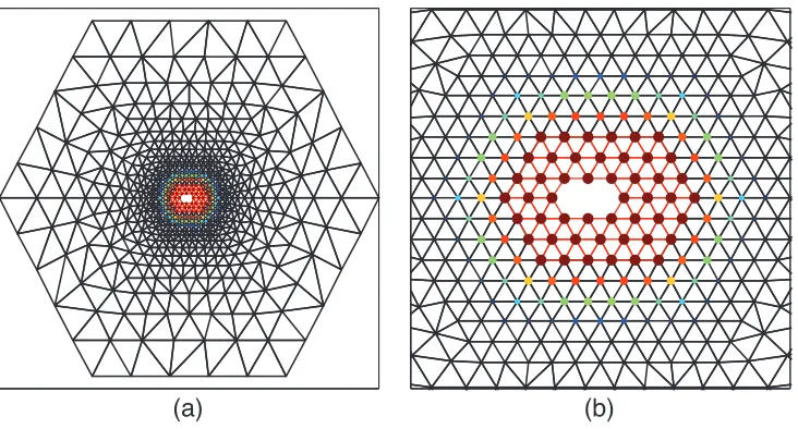
Fig. 1_{. Computational domain, finite element grid, and atomistic region as used in the}

con-struction of the BQCE and BGFC schemes. The size and color of the spheres in(b)indicate the value of the blending function (large/red stands forβ= 0).

The “renormalization” (2.4) ofEais the basis for proving thatEais well-defined on the energy spaceU [8].

2.3. Continuum model. Suppose that the site potentials are homogeneous outside the defect core, and let Φhom

a be the associated globally homogeneous site potentials for the homogeneous lattice; cf. section 2.2.

To formulate atomistic-to-continuum coupling schemes we require a continuum model compatible with (2.2) defined through a strain energy functionW :Rd×d_→R. A typical choice in the multiscale context is the Cauchy–Born model, which is defined via

W(_F) := det_A−1Φhom₀ (_Fx),

which represents the energy per unit volume in the homogeneous crystal _FΛhom = FAZd_{. The associated strain energy difference is denoted byW(G) :=W(I+G)−W(I).} 2.4. Standard blending scheme. To formulate the BQCE scheme as intro-duced in [26, 14] and analyzed in [10] we begin by defining a regular simplicial finite element grid T_h with nodes X_h, with the minimal requirement that X_h∩B_Rdef = Λ∩B_Rdef (that is, the defect core is resolved exactly). Let DOF := #X_h. Let Ω_h:=T_h ⊃B_Rc, withRc≥Rdef the resulting computational domain, and let the space of coarse-grained admissible displacements be given by

Uh:=

v_h∈C(Rd;Rd)v_h is piecewise affine with respect toT_h, andv_h|_Rd_\Ω_h= 0

.

LetQ_hdenote the P0 midpoint interpolation operator, so that_Ω

hQhfis the midpoint rule approximation to_Ω

hf.

Further, letβ ∈C2,1_(Rd_{) withβ = 0 inB}

Ra withRdef ≤Ra < Rc and β= 1 in Rd_\Ω

h; then we define the BQCE energy functional (see Figure 1)

Eb_(u

h) :=

a∈Λ_∩Ω_h

(1−β(a))Φ_a(u) +

Ω_h

Q_hβW(∇u_h).

The BQCE problem is to compute

(2.7) ub_h∈arg minEb(v_h)v_h∈U_h.

2.5. Review of error estimates. We present a formal review of error esti-mates for the BQCE scheme established in [14, 10]. This discussion will motivate our construction of the BGFC scheme in the next section.

Under a range of technical assumptions onT_h and β, it is shown in [10] that if

ua _{is a strongly stable (positivity of the hessian) solution to (2.3), and (β,T}

h) are “sufficiently well-adapted toua_{,” then there exists a solutionu}b

h to (2.7) such that (2.8)

∇ub_h− ∇u¯a_L2 ≤C1∇2β_L2+C2

βh∇2u˜a_L2(Ω_h)+∇u˜a_L2(Rd_\BRc_/2)

+. . . ,

where “. . .” denotes formally higher-order terms, ¯ua denotes a P1 interpolant on the atomistic grid Λ,and ˜ua denotes aC2,1-conforming interpolant on the atomistic grid Λ (intuitively,∇ju˜a,j ≥2, measure the local regularity ofua; see section 5 and [10] for more details). The constants depend on (derivatives of) Φ_a, a∈Λ,in a way that we will discuss in more detail below.

The termβh∇2_u˜a

L2(Ω_h)measures the finite element approximation error, while

the term ∇u˜a

L2(_Rd_\BRc/2) measures the error committed by truncating to a finite computational domain. Exploiting the generic decay rates [8]

|∇j_˜ua_(x)||x|1−d−j _{forj= 0, . . . ,3 and}

|∇j_¯ua_(x)||x|1−d−j _{forj= 0,1,} (2.9)

these terms can be balanced by ensuring that Rc _{≈ (R}a₎d/2+1 _{and that the mesh}

is coarsened according to h(x)≈(|x|/Ra)3/2 (see [21] for the two-dimensional (2D) case; the three-dimensional (3D) case is an immediate extension), which yields

βh∇2u˜a_L2(Ω_h)+∇u˜aL2(_Rd_\B

Rc/2)(DOF)

−1/2−1/d_.

By contrast, the term∇2_β

L2 is due to the (smeared) ghost forces, and even an optimal choice ofβ (balanced against the atomistic region radiusRa_{) yields only}

(2.10) ∇2β_L2 ≈(DOF)1/2−2/d.

To see this we note that a quasi-optimal choice is β(x) =B(r), where B is a radial spline with B(r) = 0 forr≤Ra andB(r) = 1 forr≥Rb∈(Ra, Rc) (see [26, 14] for in-depth discussions). A straightforward computation (assumingRb_Ra_{; the case}

Rb_Ra_{is similar) then shows that∇}2_β2

L2≈(Rb)d−1(Rb−Ra)−3+ (Rb−Ra)d−4, which is optimized subject to fixing the total number of degrees of freedom (DOF) if

Rb_−Ra_≈Ra_{. This yields precisely (2.10).}

In summary, for this simple model problem, the BQCE scheme’s rate of conver-gence,

∇ub_h− ∇u¯a_L2 (DOF)1/2−2/d,

is the same in two dimensions and worse in three dimensions than a straightforward truncation scheme, in which the atomistic model is minimized over a finite computa-tional domain (see [8]). Analogous results hold also for dislocations.

2.6. The BGFC scheme. The motivation for the BGFC scheme is to optimize the coefficientC1 in (2.8). An investigation of the analysis in sections 6.1 and 6.2 in

[10] reveals that a simple upper bound is

C1 sup

a∈Λ_∩supp(β)

sup b∈Λ_\{a}

∂Φa(y)

∂y(b) |y=x+u

.

(As a matter of fact, this form ofC1 requires a minor modification of the remaining

error estimates [10]; however, we use it only for motivation.)

The idea is to “renormalize” the interatomic potential so that δΦ_a(x) = 0 for

|a| sufficiently large, which would then ensure that|∂_y(b)Φa(x+u)||u(b)−u(a)|, and hence would yield additional decay of the constant C1 as the atomistic region

increases.

Recalling the discussion in section 2.2 we note that δΦ_a(x) = 0 for all a ∈ Λ. Thus, if we apply the blending procedure to the renormalized atomistic energy (2.4), then we would obtain a new constantC₁, with

C₁ sup a∈Λ∩supp(∇β)

sup b∈Λ\{a} rab≤rcut

∂_y(b)Φ_a(x+u)

= sup

a∈Λ_∩supp(_∇β)

sup b∈Λ_\{a} rab≤rcut

∂_y(b)Φa(x+u)−∂y(b)Φa(x)

C2∇u¯a_L∞(Rd_\BRa_−2rcut)(R a

)−d,

where the second-to-last inequality is true for sufficiently large Ra and the last in-equality follows from the decay estimate given in [8, Thm. 3.1]. We therefore obtain

C₁∇2β_L2 (DOF)−1/2−2/d, (2.11)

which not only balances the best approximation error but is even dominated by it. To summarize, the BGFC energy (difference) functional reads

(2.12) Ebg(u_h) := a∈Λ_∩Ω_h

(1−β(a))Φ_a(u_h) +

Ω_h

Q_hβW(∇u_h)+Lren, u_h,

where Φ_a is defined in (2.5),Lrenis defined in (2.6), andW(_F) :=W(_I+_F)−W(_I)−

∂W(_I) :_F. The associated variational problem is

(2.13) ubg_h ∈arg minEbg(v_h)v_h∈U_h.

We can further optimize the BGFC scheme as follows. IfRb_/Ra_∼casRa_{→ ∞,}

then the coupling error of the BGFC scheme scales like (Ra₎−d/2−2_{, and is therefore}

dominated by the best approximation error, which scales like (Ra₎−d/2−1_{. To reduce}

computational cost (by a constant factor), we can balance these two terms. Making the ansatzRb_−Ra_∼(Ra₎t_{fort∈(0,1), and noting that we can always constructβ} such that|∇2β|(Ra)−t, we obtain that

C₁∇2β_L2 (Ra)−d/2−3/2−1/2.

This is balanced with the best approximation rate, (Ra)−d/2−1, ift= 1/3.

We therefore conclude that ifRb_−Ra_≈(Ra₎t_{for somet≥1/3, then we expect} the BGFC scheme to obey the error estimate

∇ubg_h − ∇u¯a_L2(Ra)−d/2−1≈(DOF)−1/2−1/d.

We shall make this rigorous for a slightly simplified formulation in section 5, where we will also prove an energy error estimate.

2.7. Connection to ghost force correction and generalization. Consider, for simplicity, the case when Φhom

a ≡ Φa, i.e., the crystal is homogeneous. In this case,Lren_{≡0 as well. Moreover, we can rewrite the BGFC scheme as follows:}

Ebg_(u

h) =Eb(uh)−

a∈Λ

(1−β(a))δΦ_a(0), u_h −

Rd

Q_hβ∂W(0) :∇u_hdx

=Eb(u_h)− δEb(0), u_h

=Eb(u_h)− δEb(0)− Fbqcf(0), u_h,

(2.14)

where Fbqcf _{is the BQCF operator defined in [9], andF}bqcf_{(0) = 0 (this}

nonconser-vative a/c coupling has no ghost forces). Thus, we see that the renormalization step Φ_a Φ_a (cf. (2.2) and (2.5)) is equivalent to the dead load ghost force correction scheme of Shenoy at al. [24], applied for a blended coupling formulation and in the reference configuration.

This immediately suggests the following generalization of the BGFC scheme:

(2.15) Ebg(u_h) :=Eb(u_h)−δEb(ˆu_h)− Fbqcf(ˆu_h), u_h−uˆ_h,

where ˆu_h is a suitable reference configuration, or “predictor,” that can be cheaply obtained.

We will explore this alternative point of view in future work, in particular with an eye to applications involving cracks and edge dislocations. Note that this general-ization cannot be written within the renormalgeneral-ization formulations.

3. Numerical tests.

3.1. Model problems. Our prototype implementation of BGFC is for the 2D triangular latticeAZ2 defined by

A=

1 cos(π/3) 0 sin(π/3)

.

To generate a defect, we removekatoms

Λdef

k :=

−(k/2 + 1)e1, . . . , k/2e1

ifkis even,

Λdef

k :=

−(k−1)/2e1, . . . ,(k−1)/2e1

ifkis odd,

to obtain Λ :=AZ2_\Λdef

k . For small k, the defect acts like a point defect, while for largekit acts like a small crack embedded in the crystal. In our experiments we shall considerk= 2 (di-vacancy) andk= 11 (microcrack), following [14, 9, 23].

The site energy is given by an EAM (toy) model (3.1) [2], for which Φis of the form

Φ(y) = ρ∈R()

φ|D_ρy()|+F_ρ∈R()ψ|D_ρy()|,

(3.1)

with φ(r) = [e−2a(r−1)−2e−a(r−1)], ψ(r) =e−br,

F( ˜ρ) =c( ˜ρ−ρ˜0)2+ ( ˜ρ−ρ˜0)4

,

with parametersa = 4.4, b = 3, c = 5,ρ˜0 = 6e−b. The interaction range isR() =

Λ∩B2(), i.e., next nearest neighbors in hopping distance.

To construct the BQCE and BGFC schemes, we choose an elongated hexagonal domain Ωa _{containingK layers of atoms surrounding the vacancy sites, and the full}

computational domain Ω_hto be an elongated hexagon containingRc _{layers of atoms}

surrounding the vacancy sites. The domain parameters are chosen so that Rc ₌ 1

2(R

a₎2_{. The finite element mesh is graded so that the mesh size function h(x) =}

diam(T) forT ∈T satisfies h(x)≈(|x|/Ra)3/2. These choices balance the coupling error at the interface, the finite element interpolation error, and the far-field truncation error [8, sect. 5.2]. Recall, moreover, that DOF := #X_h.

The blending function is obtained in a preprocessing step by approximately min-imizing∇2β_L2, as described in detail in [14].

We implement the equivalent ghost force removal formulation (2.14) instead of the “renormalization formulation” (2.12).

3.1.1. Di-vacancy. In the di-vacancy test two neighboring sites are removed, i.e.,k= 2. We apply 3% isotropic stretch and 3% shear loading by setting

B:=

1 +s γII

0 1 +s

·F0,

where_F0∝I minimizesW,s=γII= 0.03.

3.1.2. Microcrack. In the microcrack experiment, we remove a longer segment of atoms, Λdef

11 ={−5e1, . . . ,5e1}, from the computational domain. The body is then

loaded in mixed modes I and II by setting

B:=

1 γII

0 1 +γI

·F0,

where_F0∝I minimizesW, andγI=γII= 0.03 (3% shear and 3% tensile stretch).

3.2. Methods. We test the BGFC method with blending widths K := Rb− Ra_=(Ra₎1/3_{and withK =R}b_−Ra _=Ra _{(here, the blending width denotes the}

number of hexagonal atomic layers in the blending region). The BGFC scheme is compared against the following three competitors previously considered in [14, 9, 23]:

• BQCE: blended quasi-continuum method, implementation based on [14], with most details described in section 2.4.

• GRAC: sharp-interface consistent energy-based a/c coupling [23].

• BQCF: blended force-based a/c coupling, as described in [9]. Energies of BQCF are computed using BQCE (i.e., the BQCE energy is evaluated at the BQCF solution).

3.3. Results. We present two experiments, a di-vacancy (k= 2) and a micro-crack (k= 11). For each test, we choose an increasing sequence of atomistic region sizesRa, followed by the quasi-optimal choices of Rb,Ω_h, β as described above.

For both experiments we plot the absolute errors against the number of DOF, which is proportional to computational cost, in theH1-seminorm, theW1,∞-seminorm, and the (relative) energy.

The results are shown in Figures 2, 3, and 4 for the di-vacancy problem and in Figures 5, 6, and 7 for the microcrack problem.

In the first experiment, we are able to clearly observe the predicted asymptotic behavior of the a/c coupling schemes, while in the second experiment we observe a significant preasymptotic regime, where the analytic predictions become relevant only at fairly high resolutions.

Fig. 2_{.Convergence rates in the energy-norm (the}H1_{-seminorm) for the di-vacancy benchmark} problem described in section3.1.1.

In all error graphs, we clearly observe the optimal convergence rate of BGFC, together with the other consistent methods GRAC and BQCF, while BQCE has a suboptimal rate. Recall, however, that the BGFC scheme comes with the following added advantages: over GRAC it is straightforward to construct, and over BQCF it is energy-based.

4. Extensions. It is possible to extend the formulation of the BGFC scheme to a much wider range of problems, including, e.g., multiple defect regions, problems with surfaces (e.g., nano-indentation, crack propagation), complex crystals, or higher-order finite elements. We now present a range of such generalizations, arguing again only formally.

4.1. Higher-order finite elements. We have seen in section 2.6 that in the BGFC scheme applied to point defects, the approximation error dominates the blend-ing (couplblend-ing) error. This particular bottleneck is relatively straightforward to remove by increasing the order of the finite element scheme and the size of the continuum region. The following discussion is motivated by [3].

Fig. 3_{. Convergence rates in the} W1,∞_{-seminorm for the di-vacancy benchmark problem} de-scribed in section3.1.1.

Fig. 4.Convergence rates in the relative energy for the di-vacancy benchmark problem described

in section3.1.1.

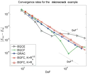
Fig. 5_{.Convergence rates in the energy-norm (the}H1_{-seminorm) for the microcrack benchmark} problem withΛdef

11 described in section3.1.2.

Fig. 6.Convergence rates in theW1,∞-seminorm for the microcrack benchmark problem with Λdef

11 described in section3.1.2.

Fig. 7_{. Convergence rates in the relative energy for the microcrack benchmark problem with}

Λdef

11 described in section3.1.2.

We construct the computational domain and finite element mesh in the same way as in sections 2.6 and 3. We decomposeT_h=T_h(P1)∪ T_h(P2), where

T(P1)

h =

T ∈ T_hβ|_T <1,

and replaceU_hwith the approximation space

U(2)

h :=

u_h∈C(Rd;Rd) u_h|_T is affine forT ∈ T_h(P1),

u_h|_T is quadratic forT ∈ T_h(P2), and (4.1)

u_h= 0 inRd\Ω_h.

That is, we retain the P1 discretization in the fully refined atomistic and blending region where Λ and X_h coincide, but employ P2 finite elements in the continuum region. To ensure stability, the quadrature operatorQ_h (previously midpoint inter-polation) must now be adjusted to provide a third-order quadrature scheme (e.g., the face midpoint trapezoidal rule) so that ∇u_h⊗ ∇u_h foru_h ∈U_h(2) can be integrated exactly.

The resulting P2-BGFC method reads

u_h∈arg minEbg(u_h)u_h∈U_h(2).

4.1.1. Convergence rate. The blending error and the Cauchy–Born model-ing error contributions to the P2-BGFC method remain the same as those for the P1-BGFC method, C₁∇2_β

L2 (Ra)−d/2−2; see (2.11) in section 2.6. Only the

approximation error component must be reconsidered. It is reasonable to expect (and we make this rigorous in section 6; interestingly, this is a nontrivial generalization) that the best approximation error contribution can be bounded by

h2∇3u˜a_L2(Ω_h\BRa)+∇u˜aL2(_Rd_\BRc /2),

where the first term is the standard P2 finite element best approximation error and the second term is the far-field truncation error.

Choosing h(x) ≈ max(1,(|x|/Rb₎3/2_{) and an increased continuum region R}c _≈

(Ra₎1+4/d_{, a straightforward computation, employing the generic decay rates (2.9) for} point defects, shows that the two terms are balanced and bounded by

h2∇3u˜a_L2(Ω_h\BRa)+∇u˜a_L2(Rd_\BRc /2)

∞

Ra rd−1

r Ra

3

r−2d−4dr

1/2

+(Rc)−d/2

(Ra)−d/2−2≈(DOF)−1/2−2/d.

It is possible to make this construction without violating the necessary mesh regularity required to obtain the stated finite element approximation error; see [16] for further discussion.

Thus we (formally) obtain

∇ubg_h − ∇u¯a_L2(Ra)−d/2−2≈(DOF)−1/2−2/d.

It is particularly interesting to note that the Cauchy–Born modeling error contri-bution is also bounded by

∇3_u˜a

L2(Ωh\BRa)+∇2u˜a2_L4(Ω_h\BRa)(R

a₎−d/2−2_≈(DOF)−1/2−2/d_,

and one may expect that this bound is optimal in most cases. Thus, we see that for the P2-BGFC method, all three error components (coupling error, approximation error, Cauchy–Born modeling error) are balanced in the energy-norm. In particular, this means that, for point defects, the P2-BGFC scheme is quasi-optimal among all a/c coupling methods that employ the Cauchy–Born model in the continuum region.

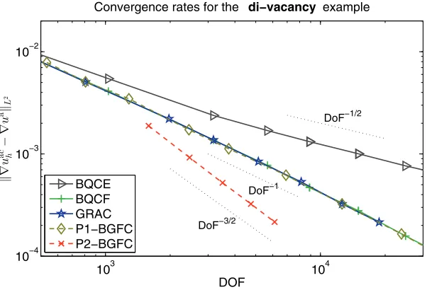
4.1.2. Numerical experiment. We test the P2-BGFC method with blending widths K := Rb_−Ra _{= R}a _{and R}c _{= (R}a₎3_{. In Figure 8, for the di-vacancy}

benchmark problem, we show an energy-norm convergence rate of P2-BGFC together with BQCE, BQCF, GRAC, and P1-BGFC with K := Rb_−Ra _=(Ra₎1/3_{. The}

predicted rate (DOF)−3/2 _{is justified by the numerical results.}

4.2. Screw dislocation. We briefly demonstrate how the BGFC scheme may be formulated for simulating a screw dislocation. The ideas are a straightforward combination of those in [8] and section 2 of the present paper, and thus we only present minimal details.

For the sake of simplicity, we restrict the discussion and implementation to nearest-neighbor interaction and antiplane shear motion, following [8, sect. 6.2]. That is, we define Λ = Λhom_=AZ2_{, where}

A=

1 cos(π₃) 0 sin(π₃)

and R={_Qj₆e1|j= 0, . . . ,5}

is the set of interacting lattice directions. (Note that Λhom _{is in fact the projection}

of a bcc crystal along the (111) direction.) Admissible (antiplane) displacements are mapsy: Λ→R.

103 104 10−4

10−3 10−2

DOF

∇

u

ac h

−

∇

u

a

L

2

Convergence rates for the di−vacancy example

BQCE BQCF GRAC P1−BGFC P2−BGFC

DoF−3/2

DoF−1

DoF−1/2

Fig. 8.Convergence rate of P2-BGFC in the energy-norm (H1-seminorm) for the di-vacancy benchmark problem described in section3.1.1.

The site potential is now a map Φ_a∈C3_(R6_{), i.e., Φ}

a(y) is a function of (y(b)−

y(a))_b∈a+R. To admit slip by a Burgers vector (we assume the Burgers vector is

(1,0,0)), we assume that Φ_a(y) = Φ_a(z) whenevery−z: Λ→Z.

A screw dislocation is enforced, e.g., by applying the far-field boundary condition

y(a)∼ylin(a) := ₂1_πarg(a−ˆa) as |a| → ∞,

where ylin _{is the linearized elasticity solution and ˆa is an arbitrary shift of the}

dislocation core. The model of section 2 can be extended by defining Φ_a(u) := Φ_a(ylin_+u)−Φ

a(ylin),and Ea(u) :=

a∈ΛΦa(u). With this modification the exact model still reads as (2.3); see [8] for details.

To define the BGFC scheme we renormalize Φ_a a second time,

Φ_a(u) := Φ_a(ylin+u)−Φ_a(ylin)− δΦ_a(0), u,

which gives rise to the BGFC functional defined by (2.12). Note thatLren_{≡0 in this}

case. The resulting BGFC scheme is still given by (2.13). Remark 1. _{(1) It is tempting to define}

Φ_a(u) := Φ_a(ylin+u)−Φ_a(ylin)− δΦ_a(ylin), u,

which seemingly has advantages in terms of error reduction. However, (i) it has the disadvantage of having to evaluate a nontrivial functionalLren, u, for which a new scheme must be developed; and (ii) the Cauchy–Born modeling error is already dominant in the dislocation case, which means that no further improvements can in fact be expected.

(2) However, taking the alternative view presented in section 2.7, we may (re)define the BGFC scheme as in (2.15), where we note that now the predictor ylin

is used for the dead load ghost force removalwithoutcreating long-ranging residual forces in the continuum region. This may indeed lead to a (moderate) improvement,

which we will analyze in future work, together with applications to edge dislocations, where the “renormalization formulation” seems less straightforward. (We note again that if the “predictor” is not homogeneous, then the GFC and renormalization for-mulations are no longer equivalent.)

(3) Employing P2 finite elements in the dislocation case does not give higher accuracy, as the rate with P1 elements is already optimal.

4.2.1. Convergence rate. Suppose that the setup of the computational geom-etry is as in section 2, with the only exception that we now need to take a coarsening rate h(x) ≈ |x|/Ra_{, due to the quadrature error (see [10]). This only marginally}

modifies the analysis.

It is shown in [8, Thm. 3.1] under natural technical conditions that if a minimizer

ua_{of the screw dislocation problem exists, then}

|∇j_y

0(x)||x|2−j and |∇ju˜a(x)||x|−1−jlog|x|.

A QNL-type ghost force free scheme (e.g., geometric-reconstruction–based [23]) is then expected to have an error of the order of magnitude of (see [8, sect. 5.2] for details)

∇¯ua− ∇uqnl_{h L}2h∇2u˜a_L2(Ω_h\BRa)+∇u˜aL2(_Rd_\BRc/2) +∇2(y0+ ˜ua)_L2(Ωi)+. . .

(Ra)−2(logRa)1/2+ (Ra)−3/2≈(DOF)−3/4,

whereuqnl_h denotes the solution of such a scheme,∇2_(y

0+ ˜ua)_L2(Ωi)is the interfacial

coupling error (cf. [18]), and we denoted again several dominated terms by “. . .”. We observe that, for QNL-type methods, the coupling error dominates the estimate.

Following the analysis in [10] and sections 2.6 and 5, we can obtain

∇u¯a− ∇ubg_{h L}2∇2β_L∞∇(y0+ ˜ua)_L2(Ωb)+ best approx.err.+. . .

(Rb−Ra)−2logRb/Ra1/2+ (Ra)−2(logRa)1/2.

We observe that with Rb_−Ra _≈(Ra₎α _{the two errors are balanced for α= 1, i.e.,}

Rb_−Ra _{≈ R}a_{, and that in this case we obtain the “optimal rate” (i.e., the best}

approximation error rate)

∇u¯a− ∇ubg_{h L}2(Ra)−2(logRa)1/2≈(DOF)−1(log DOF)1/2.

Thus, we conclude that the BGFC scheme leads to a better rate of convergence than the QNL-type scheme. This is particularly encouraging as the latter is often assumed optimal among energy-based a/c coupling schemes.

Remark 2. _{We note that the Cauchy–Born modeling error for the screw} disloca-tion example is bounded, in terms ofy=y0+u, by

∇3_y˜

L2(Ω_h\BRa)+∇2y˜2_L4(Ωh\BRa)(R

a₎₋2_≈(DOF)−1_.

Thus, up to logarithmic terms, the best approximation and blending errors are both balanced with the Cauchy–Born modeling error, which is a lower-bound for a/c cou-plings based on local continuum models. In this sense, the BGFC method isoptimal for screw dislocations as well.

102 103 104 10−4

10−3 10−2

DOF

∇

u

ac h

−

∇

¯

u

aL

2

Screw Dislocation Test : Geometry Error

GRAC−2/3 RBQCE

∼ (DOF)−3/4

∼ (DOF)−1

BGFC

Fig. 9_{. Convergence of the QNL-type GRAC-2}/_{3 [22]and of the BGFC schemes for an}

an-tiplane screw dislocation problem.

4.2.2. Numerical experiment. Replicating the setting from [8, sect. 6.2], we use a simplified EAM-type interatomic potential (cf. (2.1)), given by

Φ_a(y) :=G

b∈a+R

φ(y(b)−y(a))

, where G(s) = 1 +1₂s2,

and φ(r) = sin2πr.

Note that, in this case, the BQCE and BGFC methods are in fact identical since

δΦ_a(0) = 0. (This is an artefact of the antiplane setting.)

We employ the same constructions of the computational domain as in the point defect case described in section 3, but without vacancy sites.

In Figure 9 we compare the GRAC-2/3 method (cf. [22]) with the BGFC scheme. We observe numerical rates that are close to the predicted ones, and in particular also the moderate improvement of BGFC over GRAC-2/3 suggested in the previous section.

4.3. Complex crystals. To formulate the BGFC scheme for complex crystals, we return to the point defect problem addressed in section 2.

4.3.1. Atomistic model. Each lattice site may now contain more than one atom (of the same or different species). For simplicity suppose there are two atoms per site, which we call species 1 and species 2. The deformation of the lattice is now described by a deformation field y : Λ → Rd and a shift p : Λ → Rd. The deformed positions of species 1 are given byy1(a) :=y(a),and those of species 2 by

y2(a) :=y(a) +p(a),a∈Λ. Lety:= (y, p). The site energy is now a function

Φ_a(y) = Φ_a y_i(b)−y_j(a)_i,j=1,2

b∈Λ

.

At present there exists no published regularity theory for complex lattice de-fects corresponding to [8], which we employed in the discussion in section 2, and the following discussion is therefore based on unpublished notes [19, 17] and reasonable assumptions.

Let Φhom_a be the site energy potential for the defect-free lattice; then we assume that there is an equilibrium shift p0 such that x := (x, p0) is a stable equilibrium

configuration. By this, we mean that for all v = (v, r) with v, r : Λhom → Rd compactly supported,

a∈Λ

δΦ_a(x),v= 0 and a∈Λ

δ2Φ_a(x)v,v≥c0

|v|2_U +r22

;

that is, the configuration must also be stable under perturbations of the shifts. This corresponds in fact to the classical notion of stability in complex lattices; see [7] and references therein.

Then we define the energy-difference functional

Ea_{(u) :=}

a∈Λ

Φ_a(u), where Φ_a(u) := Φ_a(x+u)−Φ_a(x).

It can again be shown thatEa_{is well-defined and regular on the space [17]}

U:=v= (v, r) : Λ→R2dv∈U, r∈2.

The exact atomistic problem now reads

ua∈arg minEa(u)u∈U.

4.3.2. The BGFC scheme. To define the BQCE and BGFC schemes, we first define the Cauchy–Born energy density by

W(_F, p) := det_A−1Φhom₀ (_Fx, p),

where Φhom

a is the site energy potential for the defect-free lattice. Further, letW(G, q) :=

W(_I+_G, p0+q)−W(I, p0).

Let the computational geometry be set up precisely as in section 2.4, and let

U_h:=u_h= (u_h, q_h)u_h, q_h∈U_h.

Note that, contrary to the usual practice, we require that both displacement and shift be continuous functions. This is necessary in order to be able to reconstruct atom positions. The BQCE energy functional, as proposed in [19], is given, foru_h= (u_h, q_h)∈U_h, by

Eb(u_h) := a∈Λ

(1−β(a))Φ_a(u_h) +

Ω_h

Q_hβW(∇u_h, q_h)dx.

Because of the loss of point symmetry in the interaction potential, there is also a reduction in the accuracy of the Cauchy–Born model [7] and in the blending scheme. Indeed, the analysis in [19] suggests that the best possible error that can be expected for the complex lattice BQCE method is

∇u¯a− ∇ub_hL2+p¯a−pb_h2 ∇β_L2+ best approx. err. + CB err.;

that is, the blended ghost force error now scales like∇β_L2. Ifd= 2, then it can be easily seen that∇β_L2 1, while ford = 3, one even gets∇β_L2 (Ra)1/2. Thus, the standard BQCE scheme cannot be optimized to become convergent in the energy-norm.

To formulate the BGFC scheme, we renormalize Φ_a andW a second time,

Φ_a(u) := Φ_a(x+u)−Φ_a(x)− δΦ_a(x),u, and

W(_G, q) :=W(_I+_G, p0+q)−W(I, p0)−∂FW(I, p0) :G−∂pW(I, p0)·q,

and define the BGFC energy functional

Ebg(u) := a∈Λ

(1−β(a))Φ_a(u) +

Ω_h

Q_hβW(∇u, q)dx+Lren,u,

where Lren _{is the linear functional correcting the forces in the defect core, defined}

analogously toLrenin section 2.6. The BGFC scheme reads

(4.2) ubg_h ∈arg minEbg(v)v∈U_h.

4.3.3. Convergence rate. While we leave a rigorous convergence theory for (4.2) to future work, we can still speculate what rate of convergence may be expected. Arguing analogously to sections 2.6 and 5, we now observe that the error due to the blended ghost forces can be bounded by

∇u¯a− ∇ubg_{h L}2+p¯a−pbg_{h L}2∇β_L∞∇u¯a_L2(Ωb)+p¯aL2(Ωb)

+ best approx. err. + Cauchy–Born err.

It is reasonable to expect that the regularity for the deformation fieldsy1, y2is similar

as for simple lattices (indeed, this is the premise of the complex lattice Cauchy–Born rule) and therefore the best approximation error is of the same order, i.e., (Ra₎−d_. The Cauchy–Born modeling error can also be bounded by ∇2_u˜a

L2(_Rd_\BRa)+ ∇p˜a

L2(Rd_\BRa) (Ra)−d, where we assumed again the same regularity for

com-plex lattice displacement fields as that for the simple-lattice case. (Since the shift itself is a gradient, it is reasonable to expect that∇p˜a _{decays like a second gradient.)}

Thus, we are left to discuss the error due to the ghost forces. Assuming the typical decay for point defects,|∇u˜a|+|p˜a||x|−d, we obtain that for a quasi-optimal choice ofβ, satisfying∇β_L∞ (Rb−Ra)−1,

∇β_L∞∇u¯a_L2(Ωb)+p¯aL2(Ωb)

(Rb−Ra)−1(Ra)−d/2.

Upon choosingRb_−Ra_≈Ra_{, this yields the rates}

∇β_L∞∇u¯a_L2(Ωb)+p¯ a

L2(Ωb)

(Ra₎−2_{, d= 2,}

(Ra)−5/2, d= 3,

which are the best approximation rate ford= 2 and a slightly reduced rate ford= 3. We therefore conclude that the expected rate of convergence for the complex lattice BGFC scheme, for point defects, is

∇u¯a− ∇ubg_{h L}2+p¯a−pbg_h 2

(Ra₎−2_≈(DOF)−1_{, d= 2,}

(Ra₎−5/2_≈(DOF)−5/6_{, d= 3.}

With these heuristics in mind, we expect that it would be feasible to generalize the analysis in [10] and section 5 and thus obtain the first rigorously convergent a/c coupling scheme for complex crystals.

5. Analysis. For our rigorous error estimates we focus on a simplified point defect problem, following [10]. We shall cite several results that are summarized in [10] but drawn from other sources, but for the sake of convenience we will only cite [10] as a reference. A range of generalizations are possible but require some additional work, and in particular a more complex notation.

We assume Λ≡ Λhom ≡Zd (a deformation of the lattice can be absorbed into the potential), with globally homogeneous site energies with finite interaction radius in reference configuration. That is, we assume that there exists R ⊂ B_rcut ∩(Λ\

{0}), finite, and V ∈ C4((Rd)R) such that Φ_a(y) = V(Dy(a)), where Dy(a) := (D_ρy(a))_ρ∈R andD_ρy(a) :=y(a+ρ)−y(a). We assume throughout thatV is point symmetric, i.e.,−R=RandV((−g_−ρ)) =V((g_ρ)) for all (g_ρ)_ρ∈R∈(Rd₎R_.

A defect is introduced by adding an external potential Pdef _{∈ C}2_{(U), which}

depends only onDu(a),|a|< Rdef_{. The atomistic problem (2.3) now reads}

(5.1) ua∈arg minEa(v) +Pdef(v)v∈U.

We callua_{a strongly stable solution to (5.1) if there exists γ >0 such that}

δ[Ea+Pdef](ua), v= 0 and δ2[Ea+Pdef](ua)v, v ≥γ|v|2_U ∀v∈U.

The BGFC approximation to (5.1) is given by

(5.2) ubg_h ∈arg minEbg(v_h) +Pdef(v_h)v_h∈U_h,

using the notation of section 2.6.

5.1. Additional assumptions. We now summarize the main assumptions re-quired to state rigorous convergence results. All assumptions can be satisfied in practice and are discussed in detail in [10].

We assume that β ∈ C2,1_(Rd_{), 0 ≤ β ≤ 1. Let r}

cut := 2rcut+ √

d, Ωa _:=

supp(1−β) +B_r

cut, Ω

b_{:= supp(∇β) +B}

rcut and Ω

c_{:= (supp(β) +B}

rcut)∩Ωh. Then we require that there exist radiiRa_≤Rb_≤Rc_{and constants C}

b, CΩsuch that

Rb≤CbRa, ∇jβL∞ ≤Cb(Ra)−j, j= 1,2,3;

supp(β)⊃B_Ra+rcut , supp(1−β)⊂BRb−rcut;

B_Rc⊂Ωa∪Ωc and Rc≥CΩ(Ra)1+d/2.

To state the final assumption that we require on T_h, we first need to define a piecewise affine interpolant of lattice functions. If d = 2, let ˆT := {Tˆ1,Tˆ2}, where

ˆ

T1 = conv{0, e1, e2} and ˆT2 = conv{e1, e2, e1+e2}, where conv denotes the convex

hull of a set of points. If d= 3, let ˆT :={Tˆ1, . . . ,Tˆ6} be the standard subdivision of

[0,1]3_{into six tetrahedra (see [10, Fig. 1]). ThenT :=}

∈Λ(+ ˆT) defines a regular

and uniform triangulation ofRd _{with node set Λ. For eachv: Λ→R}m_{, there exists} a unique ¯v ∈C(Rd_;Rm_{) such that ¯v() =v() for all ∈ Λ. In particular, we note} that the seminorms∇v¯_L2 and|v|U are equivalent.

Our final requirement on the approximation parameters is that there exists a constantC_h such that

Th∩Ωa≡ T ∩Ωa, max T∈Th

hd_T/|T| ≤C_h,

h(x)≤C_hmax1,|x|/Ra and #T_h≤C_h(Ra)dlog(Ra).

By T_h∩Ωa _{≡ T ∩Ω}a _{we mean that if T ∈ T, T ∩Ω}a _{=∅,then T ∈ T}

h (and hence also vice versa). The conditionh(x)≤C_hmax1,|x|/Ra_{can be weakened as in the}

foregoing sections (see, e.g., [14, 21]), but for consistency with [10] we chose this more restrictive coarsening for our analysis.

We remark that (β,T_h) are the main approximation parameters, while the “reg-ularity constants” C = (Cb, Ch, CΩ) are “derived parameters.” In the following we

fix the constantsCto some given bounds, and admit any pair (β,T_h) satisfying the foregoing conditions with these constants. When we writeAB, we mean that there exists a constantCdepending only onC(as well as on the solution and on the model) but not on (β,T_h) such thatA≤CB.

5.2. Convergence result. The following convergence result is a direct exten-sion of Theorem 3.1, Proposition 3.2, and Theorem 3.3 in [10] to the BGFC method. The proof of the theorem is given in the next two sections.

Theorem 5.1. Let ua be a strongly stable solution to (5.1); then for any given set of constants C there exist C, C, Ra

0 >0 such that, for all (β,Th) satisfying the conditions of section5.1, and in additionRa_≥Ra

0, there exists a solutionu bg

h to(5.2) such that

∇u¯a− ∇ubg_{h L}2≤C(Ra)−d/2−1≤C

log #T_h #Th

1/2+1/d_, (5.3)

_Ea_(ua_)−Ebg_(ubg

h )≤C(R

a₎₋d−2_≤Clog #T_h #Th

1+2/d_. (5.4)

Remark3. (1) The only assumption we made that represents a genuine restriction of generality is that ∇j_β

L∞ (Ra)−j. We require this to prove stability of the BQCE and BGFC schemes.

(2) However, the proof of (5.4) shows that the energy error would be suboptimal if we were to choose a narrower blending region (and thus a slower rate of∇j_β

L∞ (Ra₎−sj _{for somes <1). This appears to contradict our numerical results in section} 3 and suggests that the energy error estimate may be suboptimal.

5.3. Proof of the energy-norm error estimate. To prove the result we will need to refer to another technical tool from [10], namely aC2,1_-conforming

multiquin-tic, which we use to measure the regularity of an atomistic displacement. Forv: Λ→Rm_{andi= 1, . . . , d, letd}0

iv() :=v();d1iv() := 12(u(+ei)−u(−

e_i)) and_d2

iv() :=u(+ei)−2u() +u(−ei). Lemma 2.1 in [10] states that for each

∈Λ there exists a unique multiquintic function ˜v:+ [0,1]d_→Rm_{defined through} the conditions

∂α1

x1 · · ·∂

αd

xdv˜() =dα11· · ·dαd_d v() ∀ ∈+{0,1}d, α∈ {0,1,2}d, α∞≤2,

and, moreover, that the resulting piecewise defined function ˜v∈C2,1(Rd;Rm). We begin the proof of Theorem 5.1 by noting that the renormalized site energy potential

V(Du) :=V(R+Du)−V(R)− δV(R), Du

is an admissible potential for [10, Thm. 3.1]. Further, the conditions we put forward in section 5.1 are precisely those needed to apply [10, Thm. 3.1] withV replaced by

V, thus treating BGFC as a simple BQCE method. Hence, we obtain that, under the conditions of Theorem 5.1, there exist a solutionubg_h to (5.2) and constantsC1, C2

depending only onC, but independent of the approximation parameters, such that

∇u¯a− ∇ubg_{h L}2≤C1∇2β_L2+C2

∇u¯a_L2(_R2_\BRc

/2)+h∇

2

˜

ua_L2(Ωc)

+h2∇3u˜a_L2(Ωc)+∇2u˜a2_L4(Ωc)

.

(5.5)

Here we did not write out some terms that are trivially dominated by those that we did write. In the following we writeu≡ua.

The group preceded by the constant C2 cannot be further improved, but we

will analyze in more detail the group C1∇2β_L2. This term arises from both the coarsening and modeling error analyses of the BQCE scheme in sections 6.1 and 6.2 of [10] (see also the summary in section 4.3 of [10]). We will now analyze this group in more detail.

To avoid rewriting all the terms arising in the consistency analysis in [10], we will now directly refer to the notation of that paper. The terms on the right-hand side of (5.5) all arise from bounding above the terms T1, . . . ,T4 defined at the beginning of

[10, sect. 6.1]. In [10, Lems. 6.1 and 6.2], analyzing the coarsening error contributions, it is shown that

|T1|+|T2|+|T3|coarse_β +cb_h , where (5.6)

coarse_β =∂W(_I+∇u˜)∇2β_L2 and

cb_h =C2

∇u¯_L2(_R2_\BRc

/2)+h∇

2_u˜

L2(Ωc)+h2∇3u˜L2(Ωc)+∇2u˜2_L4(Ωc)

,

and we assumed, without loss of generality, that the test function is normalized. Using the fact that∂W(_I) = 0 (due to the renormalization, the reference configuration is now stress free) we therefore obtain

(5.7) coarse_β =∂W(_I+∇u˜)−∂W(_I)∇2β

L2 |∇u˜| |∇

2_β|

L2.

We now turn towards the modeling error contribution. Assuming again, without loss of generality, that the test function is normalized, we have

|T4|_Rβ_L2,

and _Rβ is a stress error function defined in [10, eq. (4.23)], but with V replaced by

V. Following the proof of [10, Lem. 6.4] we see that in [10, eq. (6.6)] it splits

|Rβ(x)| ≤ |T1|+|T2|+O(2₂)

(note the abuse of notation: these are different T1, T2 groups than in (5.6)), and it

estimates|T2|+O(2

2)cbh . The last term is given by

T1=β∂W−

∈Λ

β() ρ∈R

V_,ρ⊗ρω_ρ(−x),

where∂W=∂W(_I+∇u˜(x)),V_,ρ=V_,ρ((_I+∇u˜(x))R),andω_ρ(y) =_s1₌₀ζ¯(y+sρ) ds, with ¯ζ being the P1 hat function for the origin on the meshT. TheO(∇2β) term now arises by expandingβ,

β() =β(x) +∇β(x)·(−x) +r_β(x;),