University of Warwick institutional repository:
http://go.warwick.ac.uk/wrap
A Thesis Submitted for the Degree of PhD at the University of Warwick
http://go.warwick.ac.uk/wrap/77521
This thesis is made available online and is protected by original copyright.
Please scroll down to view the document itself.
Essays in Applied
Economics
by
Giulia Lotti
A thesis submitted for the degree of Doctor of Philosophy in Economics
Table of Contents
Table of Contents ... 4
List of Illustrations and Tables ... 6
Acknowledgements ... 9
Declaration and Inclusion of Material from a Prior Thesis ... 11
Summary ... 12
Abbreviations ... 13
1 Tough on young offenders: harmful or helpful? ... 14
1.1 Introduction ... 15
1.2 Literature Review ... 18
1.3 Background and Design ... 20
1.3.1 Youth Custody and Detention Centres ... 21
1.3.2 Young Offender Institutions ... 24
1.4 Data ... 26
1.4.1 Treatment-Control Comparisons: Balancing Tests ... 29
1.5 Empirical Strategy and Results ... 29
1.5.1 Empirical Strategy... 29
1.5.2 Results ... 31
1.5.2.1 Prison vs. harsher youth punishment ... 31
1.5.2.2 Prison vs. softer youth punishment ... 33
1.6 Robustness Checks ... 34
1.7 Conclusion ... 37
Figures and Tables ... 40
2 Empowering Mothers and Promoting Early Childhood Investment: Evidence from a Unique Preschool Program in Ecuador ... 68
2.1 Introduction ... 69
2.2 Literature Review ... 72
2.3 Background and Design ... 74
2.3.1 The Intervention ... 75
2.3.2 Design: choosing a comparison group ... 77
2.4 Data ... 78
2.4.1 Treatment-Control Comparisons: Balancing Tests ... 79
2.4.2 Entropy Balancing ... 80
2.5 Empirical Strategy and Results ... 81
2.5.1 Empirical Strategy... 81
2.5.2 Results based on Summary Indices ... 82
2.5.4 Effect on Children Outcomes ... 92
2.6 Robustness Checks ... 94
2.6.1 Evidence on Entropy Balancing ... 94
2.6.2 Additional Robustness Checks ... 95
2.7 Conclusions ... 98
3 Minimum Wages and Informal Employment in Developing Countries ...123
3.1 Introduction ... 124
3.2 Research Design ... 127
3.3 The Data ... 130
3.4 Empirical Findings ... 135
3.4.1 Baseline Specification ... 135
3.4.2 Subsamples ... 136
3.5 Robustness Checks ... 137
3.6 Conclusions ... 138
Figures and Tables ... 140
References………..178
Appendix. Details on the Dataset Construction and Sample...159
List of Illustrations and Tables
Figure 1.1. First Stage (20 bins) ... 40
Figure 1.2. McCrary Test ... 40
Figure 1.3. Second Stage (20 bins) ... 41
Appendix Figure A1. 1. Pre-Treatment Variables (20 bins) ... 59
Figure 2.1. Identification Strategy ... 102
Figure 2.2. Why control mothers did not enrol before in the program ... 103
Figure 3.1. Minimum Wage Ratio across Countries in the 1990s ... 132
Figure 3.2. Minimum Wage Ratio across Countries in the 2000s ... 133
Figure 3.3. Minimum Wage Ratio Across Countries ...141
Figure 3.4. Deviations in the Minimum Wage Ratio from Country Means by Age………..142
Figure 3.5. Deviations in the Minimum Wage Ratio from Country Means by Education….143 Figure 3.6. Deviations in the Minimum Wage Ratio from Country Means by Gender……..144
Figure 3.7. Non-Compliance and Minimum Wage Ratio in Low Educated Cohorts……….145
Figure 3.8. Non-Compliance and Minimum Wage Ratio in Highly Educated Cohorts…….146
Table 1.1. Annual Average Population in Prison Department Establishments & Certified Normal Accommodation (CNA) on 30 June by Type of Establishment in England & Wales, 1983-1985 ... 42
Table 1.2. Annual Average Population in Prison Department Establishments & Certified Normal Accommodation (CNA) on 30 June by Type of Establishment in England & Wales, 1988-1990 ... 43
Table 1.3. Monitored Activities Offered by Functional Groups of Establishments, % of Group Offering Each Activity in 1991/2 ... 44
Table 1.4. Summary Statistics ... 45
Table 1.5. First Stage - Parametric Approach ... 47
Table 1.6. Effects of Adults’ Prison vs. Youth Custody/Detention Centres (in the Next Nine Years) ... 48
Table 1.7. Effects of Adults’ Prison vs. Youth Custody/Detention Centres by Type of Offence (in the Next Nine Years) ... 49
Table 1.8. Effects of Adults’ Prison vs. Youth Custody/Detention Centres & vs. Young Offender Institutions (in the 2.5 Years Following Release) ... 50
Table 1.9. Effects of Adults’ Prison vs. Youth Custody/Detention Centres & vs. Young Offender Institutions by Type of Offence (in the 2.5 Years Following Release) ... 51
Table 1.10. Effects of Adults’ Prison vs. Youth Custody/Detention Centres (in the Next Nine Years) - Parametric Approach... 52
Table 1.11. Effects of Adults’ Prison vs. Youth Custody/Detention Centres (in the Next Nine Years) by Offence Type - Parametric Approach... 53
Table 1.12. Effects of Adults’ Prison vs. Youth Custody/Detention Centres & vs. Young Offender Institutions by Type of Offence (in the 2.5 Years Following Release) - Parametric Approach ... 54
Table 1.13. Effects of Adults’ Prison vs. Youth Custody/Detention Centres (in the Next Nine Years) - Full Sample ... 55
Table 1.14. Effects of Adults’ Prison vs. Youth Custody/Detention Centres (in the Next Nine Years) by Offence Type - Full Sample ... 56
Table 1.15. Effects of Adults’ Prison vs. Youth Custody/Detention Centres (in the Four Years Following Release) ... 57
Appendix Table A1. 2. Offence Characteristics in More Detail ... 66
Table 2.1. Mothers' Characteristics and Pre-program Outcomes (2012) ... 104
Table 2.2. Children's Characteristics before Treatment (2012) ... 105
Table 2.3. Estimated Effects on Labour Market Outcomes and Mothers’ Economic and Social Independence (2012) ... 106
Table 2.4. Estimated Effects on Labour Market Outcomes and Mothers’ Economic and Social Independence (Pooled 2012 and 2013) ... 107
Table 2.5. Estimated Effects on Mothers’ Intra-household Decision-making (2012) ... 108
Table 2.6. Estimated Effects on Mothers’ Intra-household Decision-making (Pooled 2012 and 2013) ... 109
Table 2.7. Estimated Effects on Mothers’ Outcomes by Treatment Intensity and by Treatment Heterogeneity (2012) ... 110
Table 2.8. Estimated Effects on Children’s Outcomes: Summary Indices (2012) ... 111
Table 2.9. Estimated Effects on Children’s Outcomes by Gender, by Parental Education and by Mothers’ Employment Status (2012) ... 112
Table 2.10. Correlations between Working Condition before Treatment and Reasons Why Control Mothers Did Not Apply ... 113
Appendix Table A2. 1. Fathers' Characteristics before Treatment (2012)... 115
Appendix Table A2. 2. Household Characteristics before Treatment (2012) ... 116
Appendix Table A2. 3. Balancing Tests after Reweighting with Entropy Balancing (2012) 117 Appendix Table A2. 4. Estimated Effects on Fathers’ Labour Market Outcomes (2012) .... 118
Appendix Table A2. 5. Estimated Effects on Mothers’ Care of Children (2012) ... 119
Appendix Table A2. 6. Estimated Effects on Self-esteem, Big Five Personality Traits and Fertility Choices (2012) ... 120
Appendix Table A2. 7. Estimated Effects on Fathers’ Labour Market Outcomes (Pooled data of 2012 and 2013) ... 121
Appendix Table A2. 8. Estimated Effects on Mothers’ and Children’s Outcomes by Treatment Intensity: Summary Indices (2012) ... 122
Table 3.1. Effects of MW Ratio on Share of Self-emoyed………....147
Table 3.2. Effects of MW Ratio on Share of Self-employed (Full-Time Only)…………....148
Table 3.3. Effects of MW Ratio on Share of Self-employed (Aggregate Data) ... 149
Table 3.4. Effects of MW Ratio on Share of Self-employed (Non-linear Effects) ... 150
Table 3.5. Effects of MW Ratio on Share of Self-employed (Female) ... 151
Table 3.6. Effects of MW Ratio on Share of Self-employed (Male) ... 152
Table 3.7. Effects of MW Ratio on Share of Self-employed (Young) ... 153
Table 3.8. Effects of MW Ratio on Share of Self-employed (Prime Age) ... 154
Table 3.9. Effects of MW Ratio on Share of Self-employed (Old) ... 155
Table 3.10. Effects of MW Ratio on Share of Self-employed (Low Education) ... 156
Table 3.11 Effects of MW Ratio on Share of Self-employed (High Education) ... 157
Table 3.12 Summary Statistics ... 158
Appendix Table A3.1. Effects of MW Ratio on Share of Self-employed (First Wave) .... 162
Appendix Table A3.2. Effects of MW Ratio on Share of Self-employed (Cohorts with more than 200 observations) ... 163
Appendix Table A3.3. Effects of MW Ratio on Share of Self-employed (Variable Sector <10% missing) ... 164
Appendix Table A3.4. Effects of MW Ratio on Share of Self-employed (Non-linear Effects - Female) ... 165
Appendix Table A3.5. Effects of MW Ratio on Share of Self-employed (Non-linear Effects - Male) ... 166
Appendix Table A3.7. Effects of MW Ratio on Share of Self-employed (Non-linear Effects - Prime Age) ... 168 Appendix Table A3.8. Effects of MW Ratio on Share of Self-employed (Non-linear Effects - Old) ... 169 Appendix Table A3.9. Effects of MW Ratio on Share of Self-employed (Non-linear Effects - Low Education) ... 170 Appendix Table A3.10. Effects of MW Ratio on Share of Self-employed (Non-linear
Effects - High Education) ... 171 Appendix Table A3.11. Effects of MW Ratio on Share of Self-employed (Non-linear
Effects - Cohorts with more than 200 observations). ... 172 Appendix Table A3.12. Effects of MW Ratio on Share of Self-employed (Non-linear
Acknowledgements
First, I would like to express my gratitude to my Supervisors, Professor Victor Lavy and Dr. Fabian Waldinger. Thank you for your support and guidance throughout the PhD. Your trust in me since the very beginning motivated me to give my best and made me discover that I was able to accomplish far more than I had ever hoped (e.g. the project in Ecuador, a single-authored paper, present in Uruguay, etc.). I learnt greatly from you. Talking to you was always extremely valuable, it constantly brought me back on track and pointed me in the right direction.
Besides my Supervisors, I had the privilege to meet and work with Dr. Julian Messina. Thank you for opening me the door to the world of international organizations and for your humanity, your help goes beyond the working environment. I would also like to express my appreciation to my other co-authors, Zizhong Yan and Professor Luca Nunziata, for contributing to a positive atmosphere for research with their great mood and skills. I would also like to thank Professor Sascha Becker for generously advising me throughout these years, the Head of Department, Professor Abhinay Muthoo, for his constant support, and all the staff of the Department of Economics, I benefited from you in so many different ways.
Thanks also to Professor Robin Naylor and Professor Stephen Machin for taking the time to revise my thesis and for the useful comments they gave me during the VIVA examination.
I gratefully acknowledge the financial support from the Centre for Competitive Advantage in the Global Economy (CAGE), the Royal Economic Society, the Department of Economics of the University of Warwick, Professor Lavy, Fondazione Luigi Einaudi and the World Bank that funded me and/or parts of the research discussed in this thesis.
10
Amparito, Sarah, Lucy, Rita and all the other friends from Ecuador, I met you in a very difficult moment of my life and being with you helped me to start again.
Thanks to my current and former fellow PhD students (in particular Leta, Marti, Gonzalo, Giulio, Fede, Davidino, Chris, Moni, Rocco, Ale&Julia, Ale Scops, Anik, Anna, Tina, Julia C., Fei, Mario, Guillem, Paula, etc.), my office mates (Rig, Andi, Tony, Xinxi), my housemates (Giacomo and Paolo, I know it was a tough job to bear with me!), and other friends at Warwick (Margaret, Gill, Useful, Ele Riva, Ale&Paolo, Saretta, Andre, Francy, Bronx, Fr. Harry, etc.). I am very glad I met you, you made this journey more fun and I shared with you all the daily difficulties and joys of the process.
Heartfelt thanks to my family, to whom this dissertation is dedicated as a small token of my gratitude. Since my very first day in Coventry you were there, and you kept encouraging me until the very end, always loving me the way I am, independently from my successes and failures.
Many friends helped me to walk through my path, and indirectly encouraged me to persevere in my studies. Special thanks to all of them, in particular to Achi and Susi, the fact that you exist helps me fight against my constant cynical temptations.
Declaration and Inclusion of Material from a Prior Thesis
The thesis is submitted to the University of Warwick in support of my application for the degree of Doctor of Philosophy. It has been composed by myself and has not been submitted in any previous application for any degree.
The work presented (including data generated and data analysis) was carried out by the author, even though in the cases outlined below it was based on collaborative research:
Chapter 1 Data provided by the Research, Development and Statistics Directorate of the Home Office and analysis carried out entirely by the researcher.
Chapter 2 Data entirely collected by the researcher and analysis carried out in collaboration with Professor Lavy and Zizhong Yan.
Summary
We live in a world where resources are limited and how we invest them has an impact on the citizens’ wellbeing. The goal of this thesis is to provide, through the tools of economic analysis, some insights for the optimal allocation of our resources in three different areas: economics of crime, economics of education and economics of labour.
First, societies aim at lowering crime rates and this is why a great amount of resources is spent in punishing offenders. How effective is punishment in lowering crime rates is still unclear: what are the forms of custody that deter lawbreakers from resuming their life of crime? Through a fuzzy regression discontinuity design, we show that keeping young offenders separate from their older peers and far from an overcrowded environment is beneficial only when rehabilitation is offered.
Second, empowering women and enhancing children’s early childhood development are two important objectives that are often pursued by independent policy initiatives in developing countries. Understanding the consequences of exploiting potentially beneficial complementarities in pursuing both aims together can be relevant. Through a quasi-natural experiment we evaluate a program implemented in Quito, Ecuador, that targets both. We find that women who are involved in the education of their children are empowered in different dimensions, as reflected in their higher likelihood to find full-time employment in the formal-sector and in their greater independence in intra-household decision-making. Children’s drop-out rates decrease, while school grades and scores on cognitive tests increase, particularly for girls.
Abbreviations
AVSI
The Association of Volunteers in International Service
CNA
Certified Normal Accommodation
I2D2
International Income Distribution Dataset
ILO
International Labour Organization
PelCa
Preescolar en la Casa
– Home preschooling program implemented
by AVSI
YOIs
Young Offender Institutions
MW
Minimum Wage
NGO
Non-Governmental Organization
RD
Regression Discontinuity
se
Standard Error
1
Tough on young offenders: harmful or helpful?
ABSTRACT
How harshly should society punish young lawbreakers in order to prevent or reduce their criminal
activity in the future? Through a fuzzy regression discontinuity design, we shed light on the question by
exploiting two quasi-natural experiments stemming to compare outcomes from relatively harsh or
rehabilitative criminal incarceration practices involving young offenders in 1980’s in England and
Wales. According to our local linear regression estimates, young offenders exposed to the harsher youth
facilities are 20.7 percent more likely to recidivate in the nine years subsequent to their custody, and
they commit on average 2.84 offences more than offenders who experienced prison. Moreover, they are
more likely to commit violent offences, thefts, burglaries and robberies. On the contrary, offenders who
were sent to the more rehabilitative youth facilities are less likely to reoffend in the future when
compared to offenders sent to prison. We conclude that it is effective to keep young offenders separate
from their older peers in prison, but only when they are held in institutions that are not solely focused
on punishment.
1.1
Introduction
How tough societies should be on young criminal offenders has always been at the centre of a heated debate in history. Currently the answer is still unknown, and the evidence mixed.
On the one hand, tough policies and harsh sentences may have a general deterrence effect by discouraging people from embarking on criminal activity. Severe punishment could
also have a specific deterrence effect by discouraging people who have already undertaken criminal activity from committing new crimes in the future (Galbiati et al. 2014). On the other hand, severe punishment may have instead a negative effect on offenders who are incarcerated, weakening their already fragile links with society, nourishing negative networks, and, as a result, increasing the likelihood of future criminal activity. Furthermore, keeping offenders in custody is expensive for society. In England and Wales for example, “the average annual overall cost of a prison place for 2013-14 was £36,237”, but “45% of adults are reconvicted within one year of release” (Bromley Briefings, 2015). Hence, looking for ways in which taxpayers’ resources can be spent effectively is important.
Because the subject is difficult to study, and quality evaluations are few, supporters and opponents of tough policies have often based their stances on differing views and personal opinions rather than on empirical, causal evidence.
16
To undertake the analysis, we first consider a sample of young offenders who appeared in court when 20/21 years old and were given a custodial sentence at the beginning of the decade, when these tough regimes were in place. Our first sample includes all the offenders in England and Wales who were born in three randomly sampled weeks in 1963. In total they are 558 young offenders. We observe their criminal records until they are 30 years old. Through a fuzzy regression discontinuity design, we exploit the fact that young offenders who appeared in court when below 21 years old were sent to youth custody centres and detention centres, while young offenders who were 21 or older were sent to prison. Everything else being equal, the only reason why offenders were sent to one of the two different types of custody was the age at court appearance. To capture the effects of the different custodial treatments we exploit the plausibly exogenous variation in the age at which offenders appeared in court which, in turn, determined the type of custody the offender was sentenced to. We compare the future offences of these two groups and find that young offenders who were exposed to the harsher youth facilities are 20.7 percent more likely to recidivate in the nine years subsequent to their custody, they commit on average 2.84 offences more than offenders who experienced prison, and they are also brought to court on average 1.39 times more. The crimes committed by young offenders who were exposed to a harsher regime also appear to be more serious, as suggested by the fact that in the future they are sentenced more often to prison (even though the effect is not significantly different from zero). Moreover, their felonies are not minor, but major crimes, such as violent offences, thefts, burglaries and robberies.
Thanks to the plausibly exogenous random variation in the age at court appearance we also compare the future outcomes of these two groups. We find that offenders who were sent to the more rehabilitative youth facilities are less likely to reoffend in the future when compared to offenders sent to prison, they commit fewer offences, and they are less likely to be brought to court over a 2.5-year time period, even though all of these effects are not significantly different from zero. Moreover, offenders experiencing the rehabilitative regime are sentenced to custody again 1.28 times less than offenders experiencing prison (significant at 5%), and they are significantly less likely to commit burglaries and robberies.
While prisons do not change much across the decade, the regimes in the youth custody facilities do. This setup allows us to compare the effects of experiencing a milder/harsher custody on recidivism. We conclude that keeping young offenders separate from their older peers in prison is beneficial only if they are not kept in a solely punitive regime.
Our strategy relies on the exogenous variation in the offenders’ age at court appearance, which guarantees for the continuity of the conditional expectation of counterfactual outcomes. The ability of agents (offenders, judges, police force) to partially or completely manipulate the age at court appearance would invalidate our identification strategy. If this was the case, we would observe a discontinuity in the density function of the age at court appearance around the threshold. We perform a McCrary test and show that there is no evidence of a discontinuity in the running variable (age at court appearance) around the cut-off in neither of the two cohorts.
Our results are robust to a series of other checks: different estimation techniques (parametric and non-parametric); adding control variables in the estimation; adopting different bandwidths, samples and time windows; testing for discontinuities around the cut-off in pre-treatment variables; testing for discontinuities at points different from the cut-off in the running variable.
4 we describe the data. In Section 5 we present the empirical strategy and the results. In Section 6 we conduct some robustness checks and in Section 7 we conclude.
1.2
Literature Review
The empirical literature on the general and specific deterrent effects is still scarce (Galbiati and Drago, 2014). The main reason for this research gap is the difficulty in identifying a causal link between custody conditions and crime rates. In most cases, self-selection impedes establishing connections that are anything more meaningful than correlations: the most dangerous criminals are both more likely to be sentenced to harsher custody conditions and to reoffend in the future precisely because they are intrinsically more prone to criminal activity. Therefore, whether higher reoffending rates are driven by harsher custody conditions or by the offenders’ higher propensity to recidivate cannot be distinguished.
The difficulty of identification is exacerbated by the challenges in gaining access to data on offenders at the micro level that are necessary to isolate a specific deterrence effect, and to determine the causal link between the harsh conditions of a custodial system and the offenders’ propensity to be reconvicted. Moreover, the time span over which offenders are observed is usually short.
Washington, and, as a result, the author points out that “it is certainly feasible that incarceration has an exacerbating effect in states other than Washington, which have, for instance, worse prison conditions or educational programs” (Hjalmarsson, 2009). Lee and McCrary (2009) analyse arrests in Florida and take advantage of the more punitive sanctions for offenders who turn 18. They also find support for a specific deterrence effect, but a very small one: when offenders turn 18 and the punishment is harsher (as measured by a higher-than-expected sentence length), crime rates decline by 2 percent.
20
The evidence on the specific deterrence effect is mixed mainly due to the difference in punitive treatments, targeted populations and time windows in which offenders are observed: it is hard to draw conclusions from few and diverse studies.
The literature frequently distinguishes between the effects on offenders by their age, and whether they are classified as adults or juveniles. The former are more mature and less likely to change in response to the circumstances. The latter are more vulnerable to the surrounding environment. Malleability is not a desirable or undesirable trait per se: it implies that a young individual who lives in a negative environment is more likely to be negatively affected by it; at the same time, a young individual who lives in an edifying environment is more likely to positively change. How an individual is affected in the context of custody environments might push the individual in one of two directions: either he/she will be damaged and become more likely to reoffend in the future or he/she will not be willing to engage in crime anymore to avoid experiencing custody again.
How offenders respond to the environment when they are 20 or 21 is even more uncertain: individuals at those ages fall into a gap, in that they are not considered juveniles, and yet, at the same time, they are not as mature as adults. There is no study we are aware of that looks at how 20/21 years old offenders respond to harsh prison conditions.
1.3
Background and Design
1.3.1
Youth Custody and Detention Centres
The desire to keep young offenders separate from their older peers in the prison environment gained traction at the beginning of the 20th century in England. The idea of
focusing on education rather than punishment led to the birth of a new type of youth detention centre: the borstal, an institution initially meant to guard and rehabilitate young offenders. Its name derived from the city where the first centre was opened in 1902: Borstal, Kent, England.
In 1952 detention centres were also opened to “provide a sanction for those who could not be taught to respect the law by such milder measures as fines, probation and attendance centres, but for whom long-term residential training was not yet necessary or desirable…” (Walker, 1965).
In the first decades borstals appeared to be successful. Despite their initial success, across the years, borstals did not adapt to the new, more criminally sophisticated generations, and 70 percent of the offenders released from borstals were reconvicted within two years (Warder and Wilson, 1973). More generally, crime rates, particularly among youths, rose in the 1970s, and the public attitude toward young offenders became more concerned with punishment (Pyle and Deadman, 1994).
Hence, in 1979 the conservative party pushed for the implementation of a “short, sharp shock” on young offenders in detention centres. “The theory was that if a young man who was convicted of a first crime was given a short period of intense regimented activity from morning till night, with everything done ‘at the double’, the experience would give him such a shock that he would give up any idea of a life of crime” (Coyle, 2005). The life in detention centres during the “short sharp shock” became tough, mainly as a result of the isolation it produced:
22
prisoners were able to talk to each other for only 30 minutes daily. […] The rule of silence created an atmosphere of mental isolation. At weekends that mental isolation was consolidated by long periods of physical isolation. […] Lining the corridors, awaiting barked instructions, the sullen, pale-faced boys fixed their eyes on their jailers. It was a collective stare of silenced resentment.” (Newburn, 2009)
In the same spirit, the 1982 Criminal Justice Act (CJA) abolished borstals and replaced them with youth custody centres. The name of the sentence was changed from “borstal training recommendation” to “youth custody order”, reflecting “the view that containment is more appropriate than attempts to rehabilitate via ‘training’”. The 1982 CJA “for good or ill abandons the notions that young people are sent to penal establishments for treatment or rehabilitation” (Muncie 1984). The institution of the “short, sharp shock” and the replacement of borstals with youth custody centres represented a shift from a welfare policy system targeting rehabilitation towards a justice and retributive system focused on tighter control (Muncie, 2005; Smith, 2007). Anecdotal evidence highlights the suffering that both these centres imposed on young offenders (Muncie 1984; Taylor et al 1979); “(the centres) were, if anything, more brutal jungles than the adult prisons” (Smith, 1984). The young custody centres were not imposing the “short, sharp shock”, but life in these institutions was also tough:
“If the rule of silence, heavy discipline and limited recreation created conditions of mental and physical isolation in the Detention Centre, the endemic verbal harassment and physical violence in the Young Offenders’ Institution (Youth Custody Centres) created a climate of fear and aggression. ‘Doing time’ in either regime was about negotiating and handling punitive conditions created formally (institutionally) and informally (cultural).” (Newburn, 2009)
“Staff were so stretched that inmates were now regularly locked up for 23 hours a day, and control problems were rapidly reaching crisis proportions. […] Since the centres were established the number of assaults on staff had more than doubled and there were now five times as many attacks by inmates against other inmates. Violence, bullying, drug-taking, and solvent abuse were becoming regular features of the system.”
Source: “Youth centres' reaching crisis point'”, The Guardian, May 25, 1985.
In general during the “short, sharp shock” members of staff were often cited in the news for being violent against the offenders:
“The incident1 is the latest in a series of disturbing
episodes concerning alleged staff mistreatment of youths since the Government introduced the short, sharp shock regime, with its emphasis on discipline, parades and physical activity, at all 18 detention centres in England and Wales last year. […] It seems that assaults on young people in end have become institutionalised and are viewed by some staff as an intrinsic part of the ‘short sharp shock’. […] we should not go along the road of cruelty in our prisons and turn out youths who were more aggressive when they came out of custody than they were when they went in”.
Source: Ballantyne, Aileen. “Youth centre report criticises discipline”, The Guardian, Nov 25, 1985.
“Two dossiers containing fresh allegations of assaults by prison officers on youths at ‘short sharp shock’ detention centres are to be sent to Mr Douglas Hurd, the Home Secretary. They have been prepared by the National Association of Probation Officers and the Children’s Legal Centre after several complaints from probation officers and social workers who have come into contact with boys who say they have been slapped and punched at Blantyre House in Kent and Haslar in Hampshire.”
Source: Ballantyne, Aileen. “Prison officers punched youth, Hurd told: The practice—and…;” The Guardian, Nov 24, 1986.
“Boys (in custody) are alleged to have been punched for forgetting to say “sir”, for not knowing their numbers before being given any, and for not running quickly enough. […] “We are talking about people being punched quite forcibly in the stomach, and being given quite hard slaps around the face. I have seen a boy whose lip had been split by a blow.” […] The baton they were jumping over had been raised by the instructor just as they had estimated the height of it and had started the jump. They were clipped on the ankles,
and the baton they were running under was deliberately lowered in the same way so that they were whacked on the back. […] As soon as he arrived, he said, he was subjected to racial abuse and slapped in the face with a ruler. A prison officer then punched him in the stomach and took off his belt and slapped him around his face with it.”
Source: Ballantyne Aileen. “Punching inquiry at sharp shock centre”, The Guardian, Apr 26 1985.
It is in these years that our first quasi-natural experiment takes place. As the 1982 CJA stated, if an offender was to be punished with custody in England and Wales, he/she would have been sentenced to detention/youth custody centres if he/she was below 21 years old and to prison if he/she was 21 or older. Hence, the first comparison that we will make in this paper will be between being sentenced to a normal adults’ prison, and being sentenced to a youth custody/detention centre, where the government had decided to be more punitive.
At the time, adults’ prisons were just as tough as usual. Inmates in prison, like offenders in youth custody, could be locked up for 23 hours per day, and there were very few intermittent opportunities to work, and “little or no access to educational facilities, recreation or association” (Her Majesty’s Chief Inspector of Prisons for England and Wales, 1993).
The main differences that young offenders experienced in prison rather than in youth custody/detention centres were a) the exposure to older peers (from 21 years old onwards) and b) overcrowded cells. As Table 1.1 shows, local prisons could hold up to 150 percent of the population that the facility was originally intended to allow.
1.3.2
Young Offender Institutions
Due to their failure2, in 1988 the experiments under the “short, sharp shock” regime
were abolished, and detention centres and youth custody centres were merged into young offender institutions (YOIs). The rules by which a young offender could be sentenced to a YOI rather than to a prison were the same in 1988 as in 1982: the offender needed to be below 21
2 Crime rates did not decrease, nor the propensity to recidivate of the criminals who experienced the
when convicted of an imprisonable offence, and the court needed to be satisfied that he qualified for a custodial sentence (Scanlan and Emmins, 1988, p. 98).
These rules give us the opportunity for our second quasi-natural experiment.
It is relevant for the purpose of our study to highlight that the new institutions for young offenders were not meant to be tough anymore: at the end of the ‘80s there was a switch from a punitive system for young offenders towards a rehabilitative system (Coleman and Warren-Adamson, 1992; Muncie, 1990).
The first main differences between YOIs and prisons were that young offenders in prisons were exposed to a) older peers and to b) an overcrowded environment. As Table 1.2 shows, at the end of the ‘80s local prisons could be filled with 150 percent of the certified normal accommodation, as it used to happen at the beginning of the decade. A further dissimilarity between prisons and YOIs was c) the new educational and rehabilitative target of the latter: the aim of young offender institutions was now “to help offenders to prepare for their return to the outside community.” (HC Deb 06 June 1989). The target was to be met by “providing a programme of activities, including education, training and work designed to assist offenders to acquire or develop personal responsibility, self-discipline, physical fitness, interests and skills and to obtain suitable employment after release; fostering links between the offender and the outside community; co-operating with the services responsible for the offender’s supervision after release.” (CJA 1988, rule 3). Encouraged to maintain their networks with the outside world, young offenders were entitled to send and to receive a letter once a week, and to receive a visit once in four weeks. Outside contacts with persons and agencies were also encouraged.
By contrast, the provision of educational or training opportunities was still low for inmates in prison:
“[...] for many imprisonment results not only in a loss
26
exists, can be soulless and unrelated to sentence and needs. In most cases very little is done to prepare prisoners for release and equip them for a life outside.” (Her Majesty’s Chief Inspector of Prisons for England and Wales, 1993)
Towards the end of the decade the time during which inmates were confined in their cells diminished, but to a much larger extent in YOIs than in prisons. Among all offenders in custody, inmates in open YOIs were forced to stay in their cells for the fewest hours (42 percent of weekend hours, 40 percent on weekdays), while inmates in male local prisons were locked up in their dormitories for approximately 60 percent of their time (with peaks in London of even 83 percent during weekends)3 (Her Majesty’s Chief Inspector of Prisons for England and
Wales, 1993).
The number of monitored activities provided in the establishments also differed. For example, 23 out of 35 male and female YOIs in England and Wales offered inmates the option of undertaking agricultural and horticultural work in the open air (HC Deb 30 November 1989, HC Deb 07 November 1991), and, more generally, the largest range of activities (12–15) was provided by YOIs. Table 1.3 shows that the most popular activities were usually either equally likely to be available in both prisons and YOIs or more likely to be offered practiced in the latter4.
1.4
Data
Data provided by the Research, Development and Statistics Directorate of the Home Office allow for examination of a wide range of variables: gender; ethnicity5; the type and
number of offences for which the transgressors appeared in court; the length of the sentence they were given, the disposal; whether or not they pleaded guilty; the type of proceedings (e.g.
3 The study from the Report of a Review of Regimes in Prison Service Establishments in England and
Wales is based on 64 prison establishments in England and Wales in 1991/2.
4 There were few exceptions, mainly related to activities whose availability depended on whether the
establishment had the necessary ground to host them (like Farms Party) or to Prison Service Industries and Farms (PSIF) activities, that were not necessarily good quality workshops (Her Majesty’s Chief Inspector of Prisons for England and Wales, 1993).
5 Unfortunately the variable describing the ethnicity of the offenders of the 1963 cohort has a high
summoned by police, committed to Crown Court for trial, beach of probation order, etc.); and the date of birth (day, month and year).
We are able to access the offenders’ crime records of the first (second) cohort since their birth year until 1993, which means until they are 30 (25) years old. We measure the age at which they commit their first offence to have an indication of their initial propensity to commit a crime.
We construct several outcome variables: the likelihood of being brought to court at least once in the future; the number of offences for which an individual is sent to court; the number of times the offender appears in court again6; and the number of sentences to prison.
These outcomes refer to different time spans depending on the cohort considered. For the cohort born in 1963, the future time window in which offenders are observed is nine years (or four years after release)7. Due to data constraints, we can observe the crime records of the
offenders born in 1968 for a shorter time period. In order to maximize the time span after release in which we can observe the offenders born in 1968, we only consider the offenders who are sentenced to custody for one year or less, and we restrict the sample to offenders who turned 20/21 before June 19908. This way we broaden the time window in which we observe
the future offences of the second cohort to 2.5 years after release.
6 Please note that the number of offences for which an individual is brought to court is different from the
number of times the individual is brought to court: an offender could be brought to court once for having committed multiple offences. For example, an individual who stole a car and, when escaping, broke a shop window will go to court once but he/she will be sentenced for two different offences.
7 We reduce the time window in which we analyse the future criminal records of the offenders to nine
years (instead of 10) so that the outcomes of the two groups of offenders are comparable: we could observe for 10 years the offenders in our sample who have been sentenced at age 20, but we cannot do the same with the offenders who are sentenced when 21. This is why we choose a time window of nine years to construct our outcome variables. Therefore, we measure the future offences of the offenders who are sentenced when 20 (looking at their outcomes when they are 21 to 29), and we compare them with the future offences of the offenders who are sentenced at 21 (looking at their outcomes when they are 22 to 30). Let us point out that in the nine-year time window we are also considering offenders with a sentence longer than one year, i.e. offenders who are still in custody in this period. However, as we will see later, the sentence length is balanced between offenders assigned to youth custody/detention centres, and offenders assigned to prison, meaning that the time spent in custody by offenders from the two groups is not significantly different, and consequently, should not affect the estimates. As a robustness check we will re-conduct the analysis by looking at the offences committed only in a time window where we can observe all the offenders after release. This time window will necessarily be shorter: four years. As expected, results are perfectly in line with what is found over the nine-year period.
8 We do this because we can observe offenders until December 1993, and if we limit our sample to
28
We can also observe the type of offences committed in the future: whether they are thefts, violent offences, sexual offences, burglaries/robberies, frauds, criminal damages, drug offences, minor offences or other offences. This way we can have a measure of both the quantity and quality of future crimes.
Our first (second) sample consists of all the offenders who were born in three (four) randomly sampled weeks9 of 1963 (1968), and who were sent to either youth custody/detention
centres (young offender institutions) or adults’ prisons in England and Wales when they were 20/21 years old.
The Criminal Justice Act 1982 that established the rules for youth custody and detention centres was implemented on the 24th of May 1983. We therefore include in our first sample only offenders who were 20/21 years old after that date. In total there are 558 offenders10. Of them 315 offenders were sent to adults’ prisons (our treatment group), and 243
offenders were sent to youth custody/detention centres (our control group). The Criminal Justice Act 1988, which abolished youth custody/detention centres and established YOIs, was implemented on the 1st of October 1988. Following the same reasoning, we include in our
sample offenders who appeared in court when 20/21 after that date. In total there are 297 offenders. Of them, 132 were sentenced to adults’ prisons (our treatment group), and 165 were sentenced to YOIs (our control group).
Summary statistics of the observable characteristics of offenders from both cohorts are reported in Table 1.4. Most of the offenders born in 1963 (Panel A) are male (93.2 percent), and they appeared in court for the first time when they were almost 17 years old on average. Around 90 percent of them pleaded guilty when 20/21, and they were given a sentence of
we would also observe offenders who turned 20/21 between July and December 1990, but we would examine their post-release behaviour for two years only.
9 Dates for the 1963 cohort: 3rd-9th March, 28th September-4th October, 17th-23rd December. Dates for
the 1968 cohort: 3rd-9th March, 28th September-4th October, 17th-23rd December and 19th-25th June for the
1968 cohort.
10 We exclude from the 1963 cohort offenders who committed their first crime when they were younger
approximately 9.5 months on average. The offences were: burglaries (36.7 percent), violent offences (17 percent), and thefts of different kinds (30.5 percent). Most of the offenders born in 196811 (Panel B) are male (97.3 percent) and of White European ethnicity (58.1%). The
offences committed by the 1968 cohort are also mainly burglaries (30.7 percent), violent offences (22.6 percent) and thefts (26.4 percent).
1.4.1
Treatment-Control Comparisons: Balancing Tests
We rely on a standard regression discontinuity design assumption, specifically in this case that the assignment to treatment is not correlated to individuals’ characteristics other than age. Therefore, we provide visual evidence of whether other covariates exhibit a jump around the threshold. As shown in Appendix Figure A1.1,this is not the case for any of the available observable characteristics: gender, ethnicity, birth year (the members of the groups we compare are all born in the same year), month of birth (March, June12, September/October, December),
whether they pleaded guilty, the type of offence, the age at which they committed their first offence and the proceedings types. The absence of a jump in observable characteristics around the cut-off further supports our analysis.
1.5
Empirical Strategy and Results
1.5.1
Empirical Strategy
The 1963 and 1968 cohorts are analysed separately through a fuzzy regression discontinuity (RD) design. It is a fuzzy RD because not all the offenders who should be sentenced to either prison or separate youth establishments are effectively sentenced to them. That is, 230 (160) offenders out of the 243 (164) who appeared in court when age 20 from the 1963 (1968) cohort were sent to youth custody/detention centres (young offender institutions),
11 We limit our sample of offenders born in 1968 to offenders who were given a custodial sentence of
one year maximum, which makes summary statistics of the 1968 cohort slightly different compared to the 1963 cohort.
and 297 (128) young offenders out of the 315 (132) who appeared in court when age 21 were sent to adults’ prisons. This gives us the possibility of estimating the local average treatment effects (LATE) by two-stage least squares (2SLS). The following model illustrates how.
First stage equation:
𝐷𝐷𝑖𝑖= 𝛼𝛼+ 𝑓𝑓1(𝑥𝑥�𝑖𝑖) +𝜌𝜌𝑇𝑇𝑖𝑖+𝜂𝜂𝑖𝑖
(1)
Second-stage equation:
𝑌𝑌𝑖𝑖 = 𝛼𝛼+ 𝑓𝑓2(𝑥𝑥�𝑖𝑖) +𝛾𝛾𝐷𝐷𝑖𝑖+𝑒𝑒𝑖𝑖
(1)
Where:
Yi= the outcome for individual i, i.e. the likelihood to re-offend in the future, the
number of crimes committed, the number of court appearances, the number of sentences to prison, the number of specific types of crime committed;
Di = the treatment variable, equal to 1 if individual i is sentenced to an adults’ prison,
and 0 otherwise;
Ti = 1 if individual i is 21 years old or older, and 0 otherwise; it is used as instrument
for Di.
Xi = age of individual i when sentenced, centred so that it is 0 when the individual turns
21 years old, positive if the individual is sentenced when 21 years old or older, and negative when the individual is younger than 21 years old13.
The functional forms f1 and f2 need to be correctly specified.
Our main specification is estimated through a non-parametric approach, implementing a local linear regression constructed with a triangular kernel regression14. As Lee and Lemieux
13 The centred running variable is equal to 1 the day after the offender turned 21 and -1 the day before
his 21st birthday.
14 A triangular kernel is ideal for estimating effects at the boundary (Fan and Gijbels 1996, Lee and
Lemieux 2014). Moreover, results (available upon request) are robust to using different kernels, like the uniform or Epanechnikov.
(2010) suggest, it is better not to rely on one method only, so we will also estimate equations (1) and (2) through a parametric approach. To allow for non-linearities, we use polynomials, but up to the second order only. We do not control for higher polynomials (third, fourth, etc.) of the forcing variable because it could lead to misleading results (see Gelman and Imbens (2014)). We also allow the treatment to have a different impact before and after the cut-off by including an interaction of the centred variable and the treatment variable. Finally, for a further robustness check, we also include in our parametric approach estimations control variables such as gender, month of birth, ethnicity, age at which the offender committed the first offence, sentence length, plea, proceedings and type of offence when the offender was sentenced to youth custody/detention centres/young offender institutions or adults’ prisons.
1.5.2
Results
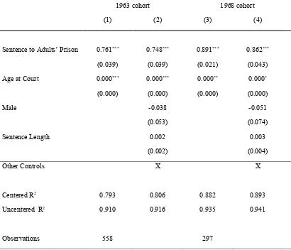
For both our cohorts, the first stages are strong: the estimated coefficients in equation (1) are 0.761 for the 1963 cohort and 0.891 for the 1968 cohort (Table 1.5), very precisely estimated. We can visualize the strength of our first stages in Figure 1.1.
1.5.2.1
Prison vs. harsher youth punishment
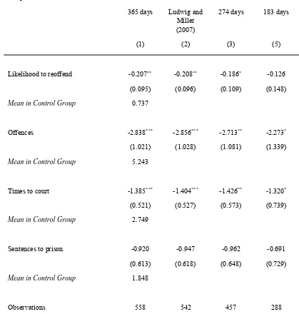
Let us begin our treatment effects analysis by looking at the future offences of the 1963 cohort through the local linear regression (Table 1.6). In the first column we report the estimated treatment effect when the bandwidth is one year on both sides15. In column (2) we
present the estimates with the bandwidth suggested by Ludwig and Miller (2007), in column (3) we restrict the bandwidth to ¾ of a year and in column (4) to half a year.
We find that young offenders who experienced custody in prison are 20.7 percent less likely to re-offend than those who were exposed to a harsher treatment over a nine-year time span. The effect is significant and does not change even when we reduce the bandwidth around
15 By this, we mean that we include in our sample young offenders who appear in court from the date of
their 20th birthday up to young offenders who are sentenced the in their 22nd birthday, i.e. +/- 1 year from
the cut-off from one year to the optimal bandwidth suggested by Ludwig and Miller (2007) or to ¾ of a year. The effect is no longer significantly different from zero at conventional significance levels only if we reduce the bandwidth to half a year. Hence, young offenders exposed to a harsher punishment are more likely to reoffend, and this is also reflected in the number of future offences they commit over the nine-year period: on average 2.84 offences more than their peers who were subject to less severe incarceration conditions. This is true across all different bandwidths. Not only young offenders who experienced the harsher treatment are more likely to be sentenced for more offences in the future, but they are also brought to court on average 1.39 times more. The two outcomes differ in magnitude because an offender can go to court once and be sentenced for more than one offence at the same court appearance.
We then investigate on the seriousness of the crimes committed in the nine subsequent years. Using the number of future sentences to prison as a proxy for severe crimes, we find that offenders who experience the tougher regime are more likely to be sentenced to prison in the future, but not significantly so. In Table 1.7, we examine the types of crimes committed, and we show that the overall effects we find are not driven by minor offences, but mainly by violent offences, thefts, burglaries and robberies. These differences between the two groups of young offenders are significant even when we restrict the bandwidth as previously detailed16. We find
no significant differences in the number of future violent crimes (such as sexual offences), or in the number of various other crimes (drug offences, minor offences, motoring offences, frauds). There seems to be an effect on criminal damage too, but it vanishes when we restrict the bandwidth around the threshold.
In summary, on the one side there are overcrowded prisons where offenders are exposed to older peers; on the other side there is a tougher than usual regime, with the main purpose to punish and shock offenders. The overall effects of the latter are more detrimental:
16 While in the first column we report the estimated treatment effect when the bandwidth is one year on
offenders who are sentenced to youth custody/detention centres are more likely to re-offend in the future, to commit a greater number of offences and to commit offences that are more dangerous for society. Through this analysis we are not able yet to disentangle the mechanisms that are driving the results.
1.5.2.2
Prison vs. softer youth punishment
We now analyse the future offences of the 1968 cohort, comparing the young individuals who were sent to the usual adults’ prisons to the ones assigned to YOIs. As we previously explained, we examine this cohort over a shorter period: 2.5 years after release. We will then re-conduct our analysis for the 1963 cohort limiting the time window to 2.5 years, and limiting the sample to offenders sentenced for one year or less. This way we can compare the results we obtain by analysing the 1963 and 1968 cohorts.
years following release, they commit on average 1.03 fewer offences, and they appear in court 0.57 times fewer. Hence, it seems that even in the short term, young offenders who experience the harsher treatment become more dangerous for society. All these estimates are significantly different from zero and, as we highlighted before, they go in the opposite direction of what we find once the harsh treatment for young offenders is abolished.
Moreover, similarly to what we found over the nine-year time window, this shorter time window still shows that violent offences and thefts constitute the types of crimes more often committed more often by offenders who experienced youth custody and detention centres (Table 1.9).
In summary, being exposed to (harsher) youth custody/detention centres makes offenders more dangerous than being exposed to prisons; while being exposed to (less harsh) YOIs makes offenders less dangerous than being exposed to prisons. Given that prisons did not experience major changes over the ‘80s, and given that the differences in the age of peers and in overcrowding rates between prisons and establishments for youth did not change significantly over time, our findings seem to suggest that it is wise to keep young offenders away from prisons, but only if they are kept in institutions with a rehabilitative purpose. If instead, young offenders are kept separate from their older peers and far from an overcrowded environment, but with the aim of punishing them, their likelihood of reoffending in the future is exacerbated.
1.6
Robustness Checks
Estimated coefficients tend to appear slightly smaller in size when control variables are included, but they are not significantly different from the coefficients estimated without control variables. In Table 1.11 we show the different treatment effects by offence type, estimated through a parametric approach: effects go in the same direction as through the non-parametric. One could worry if there were a discontinuity in the distribution of the forcing variable (the age at which offenders go to court) at the threshold (21 years). This would suggest that people (judges, police, the offenders themselves) can manipulate the forcing variable around the threshold. For example, young offenders, knowing ex-ante the harsh conditions of youth custody and detention centres, could wait to commit their crimes until they turn 21 years old. Reassuringly, the McCrary test shows no manipulation of the assignment variable for either cohort (Figure 1.2).
young offenders who went to youth custody/detention centres are significantly more likely to commit thefts, violent offences, burglaries and robberies, as we found in our original sample.
In Section 5 we analysed the future felonies of the 1963 cohort over the next nine years, even though over this time some offenders are not free from confinement, but kept in custody. If the sentence length for offenders in youth custody/detention centres and offenders in prisons were different, the main results we presented would be biased, as the number of free people facing the choice of committing (or not) new offences would be disproportionate. However, we have already seen that the sentence length is balanced, meaning that the time spent in custody by offenders from the two groups is not significantly different, and consequently, will not affect the estimates. As a robustness check we re-conduct the analysis by looking at the offences committed only in a time window where we can observe all the offenders outside of custody. The time window that enables us to conduct this analysis is four years17. As we can
see in Table 1.15, results are perfectly in line with what is found over the nine-year and 2.5-year periods: offenders who have been exposed to prisons rather than to youth custody/detention centres on average commit 1.8 fewer offences in the five years following release (-1.03 in 2.5 years following release, -2.84 in nine years); they are 35.7 percent less likely to commit offences (-31.1 percent in 2.5 years, -20.7 percent in nine years); and they appear in court almost once less (-0. 57 time in 2.5 years, -1.39 in nine years). If we then dig into the type of offences committed, we can see that they are mostly violent offences, thefts and, in this case, also criminal damage.
We also need to bear in mind that the number of offences captured in the analysis underestimates the true level of re-offending because crimes are only partially detected, sanctioned and recorded. Our estimated effects would be biased if there were a difference in
17 The time window is four years because once we exclude two offenders who have been given a sentence
of 60 months, the longest sentence we have in the sample is 48 months, i.e. four years. This means that offenders born at the latest in our sample (i.e. in December 1963) and who are sentenced to prison until
they are still 21 (i.e. at the latest December 1985, some days before their 22nd birthday) for the maximum
how easy it is to detect, sanction and record the offences of the two groups. However, we do not have any reason to believe there was.
Our first stage is very strong, but as a placebo test we also check if there are other jumps in the forcing variable. Following Imbens and Lemieux (2008) we only look at one side of the discontinuity, take the median of the forcing variable in that side and test for discontinuity. Reassuringly, we find none.
1.7
Conclusion
We use a fuzzy regression discontinuity design to analyse two quasi-natural experiments in criminal sentence of 20- and 21-year-old offenders to compare the effects of incarceration practices that are harsher or more rehabilitative in nature. The work contributes to the literature and current public debate on the most effective type of punishment to reduce crime among young offenders and to protect the citizens’ wellbeing.
We find evidence that keeping young offenders separate from their older fellows is efficient when we aim to reduce their future criminal activity. However, this is true only if the young offenders are housed in institutions that provide for their rehabilitation. Keeping young offenders in institutions with a sole punitive purpose proves to be counterproductive instead.
38
offences, thefts, burglaries and robberies. By the end of the decade punitive institutions for young offenders are abolished and substituted with more rehabilitative ones, which enables us to compare young offenders sentenced to the usual prison with young offenders sentenced to the separate educational institutions. In the 2.5 years after release, offenders held in the new educational facilities are sentenced to custody 1.28 times less than offenders kept in ordinary prisons; they are also significantly less likely to commit burglaries and robberies, suggesting that they become less of a threat for their society. They are also less likely to re-offend and they commit fewer crimes in the future, but the estimates of these effects are not significant.
Adults’ prisons do not experience major changes over the decade. Moreover, the different exposure to overcrowding and to peers between prisons and establishments for younger offenders stay the same. The only difference between the two types of custody that varies over time is the change of target in institutions for young offenders, from a punitive one to a rehabilitative one. Hence, our results imply that being kept separately from more adult criminals is positive only if the purpose of the offender’s custody is rehabilitative. If it is punitive, the lawbreaker becomes even more likely to reoffend in the future.
Our estimates hold to different robustness checks.
These results suggest that the experience of being held in punitive incarceration facilities can have negative long-term consequences on young offenders, and therefore on the entire society. The evidence is significant, with the caveat that it relates to a specific group of offenders: law breakers who are sentenced to custody when 20/21 years old. While being an interesting result per se, it cannot be generalized to juvenile or adult offenders, even though our results are in line with the literature that does not find evidence in favour of a specific deterrence effect for juveniles (Aizer and Doyle 2015) and adult offenders (Chen and Shapiro 2007, Drago and Galbiati 2011, Mastrobuoni and Terlizzese 2014).
the aim of our paper is to test for the presence of a specific deterrence effect, but we cannot draw any conclusion on the general deterrence effect: we do not know how other individuals who did not experience youth custody, detention centres, young offender institutions or adults’ prisons when 20/21 respond to the existence of these institutions.
40
Figures and Tables
Figure 1.1. First Stage (20 bins)
Notes: The figure above reports the first stages, i.e. how much of being sentenced to an adults’ prison depends
on actually being 21. The left (right) hand side refers to the 1963 (1968) cohort of the Offenders Index Cohort Data (Home Office Research, Development and Statistics Directorate). The 1963 sample includes all the offenders who were sentenced to either youth custody/detention centres or adults’ prisons when being age 20/21 at the date of court appearance. The 1968 sample includes allthe offenders who were sentenced to young offender institutions or adults’ prisons when being age 20/21 at the date of court appearance. On the x axis lies our running variable, age at court appearance, centred at 0 when age at court appearance is 21. Age at court appearance is positive (negative) when young offenders are older (younger) than 21. On the y axis the treatment dummy (equal to 1 when the offender is sentenced to prison) is plotted. The coloured areas represent the 90% confidence intervals around the separate lines of quadratic best fit plotted on the left and right hand side of the cut-off.
Figure 1.2. McCrary Test
Notes: The figure above refers to the 1963 (Panel A) and 1968 (Panel B) cohorts of the Offenders Index Cohort
Data (Home Office Research, Development and Statistics Directorate). The 1963 sample includes all the offenders who were sentenced to either youth custody/detention centres or adults’ prisons when 20/21. The 1968 sample includes allthe offenders who were sentenced to young offender institutions or adults’ prisons when being age 20/21 at the date of court appearance. The McCrary test is “a test of manipulation related to the continuity of the running variable density function” (McCrary, 2008). On the x axis lies our running variable, age at court appearance, centred at 0 when the age at court appearance is 21. Age at court appearance is positive (negative) when young offenders are older (younger) than 21. On the y axis the density function of the running variable is plotted.
0
.00
1
.00
2
.00
3
-500 0 500
0
.00
1
.00
2
.00
3
.00
4
Figure 1.3. Second Stage (20 bins)
Notes: The figure above refers to the two samples from the 1963 (Panel A) and 1968 (Panel B) cohorts of the Offenders Index
Cohort Data (Home Office Research, Development and Statistics Directorate). The 1963 sample includes offenders who were sentenced to either youth custody/detention centres or adults’ prisons when being age 20/21 at the date of court appearance and who committed their first offence when older than 14. The 1968 sample includes offenders who were sentenced to young offender institutions or adults’ prisons when being age 20/21 at the date of court appearance, whose sentence was equal or shorter than one year and who committed an offence before June 1990. On the x axis lies the variable age at court appearance, centred at 0 when age at court appearance is 21. Age at court appearance is positive (negative) when young offenders are older (younger) than 21. On the y axis the outcomes measured after release are represented: the number offuture offences, the likelihood to reoffend, the number of sentences to prison and the times the offenders go to court again. The coloured areas represent the 90% confidence intervals around the quadratic of best fit. The time span over which outcomes are observed is nine (2.5) years after release for offenders born in 1963 (1968).
Panel A – 1963 Cohort
42
Table 1.1. Annual Average Population in Prison Department Establishments & Certified Normal Accommodation (CNA) on 30 June by Type of Establishment in
England & Wales, 1983-1985
Type Of Establishment 1983 1984 1985
Average
Pop.
CNA Average
Pop.
CNA Average
Pop.
CNA
Local Prisons 15,801 10,864 15,219 10,934 16,512 10,949
Open Prisons 3,104 3,246 2,971 3,281 3,194 3,406
Closed Training Prisons 12,368 11,690 12,096 11,821 13,050 12,669
Open Youth Custody
Centres
1,425 1,557 1,390 1,613 1,351 1,496
Closed Youth Custody
Centres
5,066 5,280 5,244 5,297 5,488 5,375
Senior Detention Centres 1,144 1,550 943 1,459 968 1,341
Notes: The table reports the annual average population in the prison department establishments relevant to our paper
and their certified normal accommodation (CNA) on 30th of June in England and Wales in 1983-1985.
Table 1.2. Annual Average Population in Prison Department Establishments & Certified Normal Accommodation (CNA) on 30 June by Type of Establishment in
England & Wales, 1988-1990
Type Of Establishment 1988 1989 1990
Average
Pop.
CNA Average
Pop.
CNA Average
Pop.
CNA
Local Prisons 17,298 11,237 17,354 12,347 15,551 11,460
Open Prisons 3,141 3,312 3,252 3,700 3,187 3,496
Closed Training Prisons 15,525 16,090 16,543 17,086 16,651 17,073
Juvenile Young Offender
Institutions
293 502 330 409 285 398
Short Sentence Young
Offender Institutions
438 694 340 570 296 448
Other Open Young Offender
Institutions
1,174 1,472 976 1,456 877 1,312
Other Closed Young
Offender Institutions
5,102 5,361 4,863 5,191 4,232 4,711
Notes: The table reports the annual average population in the prison department establishments relevant to our paper
and their certified normal accommodation (CNA) on 30th of June in England and Wales in 1988-1990. Young offender institutions were established in October 1988, hence their CNA in 1988 is measured on the 30th of December.