Groovy Parity Games
Daan Kooij
University of Twente P.O. Box 217, 7500AE Enschede
The Netherlands
[email protected]
ABSTRACT
Parity games are often used for the formal verification of software systems and for the µ-calculus model-checking problem, but reasoning about them is generally hard. Mul-tiple algorithms solve parity games, but none of them do so in polynomial-time, even though it is widely believed that a polynomial algorithm exists. In this paper, we show that it is possible to model one such algorithm,priority promotion, as a series of graph transformations, and de-scribe how to do it. Subsequently, we use these graph transformations to visualise the algorithm in the formal graph transformation toolGroove, with the goal to provide researchers with a better understanding of parity games. We also model several extensions to the algorithm using recursion and non-determinism. Finally, we reflect on the results and suggest directions for future research.
Keywords
Parity games, priority promotion, visualisation, attractor computation, formal verification,µ-calculus, model check-ing, graph transformations, Groove, control program, state space exploration, non-determinism, recursion
1.
INTRODUCTION
A parity game is a perfect-information, turn-based, infinite-duration game between two players;Even andOdd. The game is depicted by a simple graph, where the vertices
V are the disjoint union of V0 and V1, and the edges
E ⊆V ×V are such that every vertex has at least one outgoing edge. VerticesV0 are controlled by playerEven,
and verticesV1are controlled by playerOdd. In addition,
every vertex has a priorityp∈Z≥0.
The game is played by moving a single token over the vertices along the edges. At every turn, the player that controls the vertex where the token resides decides along which edge the token is moved. This yields an infiniteplay. The play is won by the player with the parity of the highest priority encountered infinitely often.
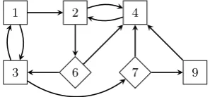
Typically, we depict a parity game as in Figure 1. The vertices controlled by Even are shown as diamonds, the vertices controlled byOdd are shown as squares, and the priorities are shown as labels on the vertices. In this game,
Permission to make digital or hard copies of all or part of this work for personal or classroom use is granted without fee provided that copies are not made or distributed for profit or commercial advantage and that copies bear this notice and the full citation on the first page. To copy oth-erwise, or republish, to post on servers or to redistribute to lists, requires prior specific permission and/or a fee.
31stTwente Student Conference on IT.July 5th, 2019, Enschede, The Netherlands.
Copyright2019, University of Twente, Faculty of Electrical Engineer-ing, Mathematics and Computer Science.
given that the token starts at a vertex with priority 1 or 3, playerOdd wins the game, asOdd can keep moving the token between the vertices with priorities 1 and 3, causing the highest priority to be encountered infinitely often to be 3. However, if the play would start at any other vertex, playerEven would win, as then the only priorities that can be encountered infinitely often are{2,4,6}, as playerEven
always selects the (6,4) edge in the vertex with priority 6.
1 2 4
[image:1.595.347.496.298.367.2]3 6 7 9
Figure 1. Example of a parity game
1.1
Related Work
In practice, parity games are often used as the back-end for the formal verification of software systems, and are closely related to the theory of formal languages and automata[11]. Parity games are used to solve modal fixpoint logics such as
µ-calculus, CTL*, CTL and LTL[5, 6, 12, 15]. Solving the model checking problem of theµ-calculus[6] is equivalent to solving a parity game[8], and the translation between them can be done in linear time[9].
Solving a parity game entails finding the winning regions and corresponding strategies for both players. A winning region of a certain player is a set of vertices from which the player wins the game independent of the choices of the other player, given that they play according to their winning strategy. Several algorithms solve parity games, such asPriority Promotion[4],Zielonka’s Algorithm[18],
Strategy Improvement[10] andSmall Progress Measures[13], most of them having a number of variations[2, 3, 17].
The priority promotion and Zielonka algorithms solve parity games by the means ofattractor computations[16]. An attractor is a set of vertices from which a certain player can ensure arrival in a given target set.
1.2
Contributions
Generally, parity games and their algorithms are hard to reason about. Currently, no algorithm solves parity games in polynomial time, even though it is believed that such an algorithm exists[1]. This is an open problem, which makes finding a polynomial solution interesting also from a theoretical perspective[3]. We refer to Czerwinski et al.[7] for an overview of recent work on this topic.
the algorithms can be visually inspected. However, because the algorithms often have many iterations before producing a solution, it is very difficult to do this manually. It would therefore be useful to have some form of automatic visuali-sation of these algorithms, but current graph visualivisuali-sation tools (such as Graphviz) are inadequate, as they do not allow for a structured inspection of many states.
Therefore, to provide a better understanding of parity game algorithms, we visualise the priority promotion algo-rithm using graph transformations[14] in the formal graph transformation toolGroove. The main reason that we use Groove as a visualisation tool, is that with Groove graph transformations can easily be defined, inspected and ap-plied on graphs. In addition, when non-determinism is introduced, a complete state space exploration can be done to explore the different runs of the algorithm. Each indi-vidual state change can be retraced, which makes Groove a useful visualisation tool for parity game algorithms.
The reasons described above let us to experiment with alternative versions of the priority promotion algorithm. In this paper, in addition to modelling the main algorithm, we also describe non-deterministic and recursive variants of the algorithm.
2.
PRIORITY PROMOTION
2.1
Main Algorithm
The first step in modelling the priority promotion algorithm as a series of graph transformations, is understanding the algorithm itself. The pseudocode of the algorithm is given in Algorithm 1.
The algorithm receives as input a parity game, and returns a dominion (a winning region) of a certain player. The algorithm is only called with vertices of the parity game that are not yet in any returned dominion. Once every vertex is part of a dominion, the winning regions of both players are known, meaning that the parity game is solved.
The algorithm itself relies on the computation ofattractors. In the algorithm, attractors are computed for vertices with a certain priority, starting with the highest priorities. Vertices in an attractor will temporarily be removed from the subgame, meaning that they will not be attracted to other attractors. If an attractor is a globally closed region for a certain player (meaning that the player can keep the token in the region, and the other player cannot move the token out of the region), this means that a dominion for a specific player is found, causing the algorithm to return.
If, on the other hand, a locally closed region for a certain player is found (meaning that the player can keep the token in the region, and the other player can only move the token out of the region to a vertex not in the subgame), that region is merged with the lowest priority escape region (meaning the region with the lowest priority where the other player can move the token from the attractor), and all of the lower priority regions are reset. Note that there always is at least one locally closed region, as the region with the lowest priority is always locally closed.
2.2
Extended Versions
In addition to the main functionality of the priority pro-motion algorithm, we also describe several extensions to the algorithm, as Groove allows us to easily make changes to certain aspects of the algorithm.
2.2.1
Non-Determinism
In its default version, the priority promotion algorithm does not have any non-determinism. However, we can
Data: parity game
Result: a dominion of a player
region:= initialize empty map from vertex to priority;
forvertex∈parity game do region[vertex] := -1 ;
priorities:= map from vertex to priority with priorities as given byparity game;
current priority := highest priority in game;
whiletrue do
// Do until dominion is found
α:= parity ofcurrent priority;
α:= parity of (current priority + 1);
subgame:= all vertices whereregion[vertex] ≤
current priority;
attractions:= attract for all vertices insubgamewhere
region[vertex] =current priority orpriorities[vertex]
=current priority;
open vertices:= all vertices ofαthat are inside
attractionsand have no edges to vertices inside
attractions;
escapes:= all successors of vertices ofαwithin
attractionsthat are outsideattractions;
locally closed :=open verticesis empty and intersection ofsubgamewithescapes is empty;
globally closed :=open verticesis empty andescapes
is empty;
if not locally closed then forvertex∈attractions do
region[vertex] :=current priority;
end
current priority := highest priority of vertices in
subgame that are not inattractions;
else if not globally closed then
current priority := lowestregion[vertex] of any vertex inescapes;
forvertex∈attractions do
region[vertex] :=current priority;
end
forvertex∈parity game do
// Reset lower regions
if region[vertex]<current priority then
region[vertex] := -1;
end end else
// Dominion for α is found
if region[vertex]6=current priority then
region[vertex] := -1;
end
attractions:= attract for all vertices inattractions;
return(attractions,α);
end end
Algorithm 1:Priority Promotion algorithm pseudocode
Using Groove, we can do a complete state space exploration to enumerate all different winning strategies produced by different attractor computations, and visually inspect the steps taken to get there.
We can also introduce non-determinism in the way that closed regions are treated. Instead of immediately promot-ing a locally closed region or returnpromot-ing a dominion, we can non-deterministically ignore them. We can then again do a state space exploration to investigate whether a solution is found faster by sometimes ignoring closed regions.
2.2.2
Recursion
At its default behaviour, whenever an attractor is deter-mined to be not closed, the current priority is simply updated to be the highest remaining priority, and a new attractor is computed. However, often a subset of the non-closed attractor is closed. We can discover this by taking as subgame the vertices in the attractor that are not open and are not attracted to the open vertices, and recur-sively execute the algorithm (finding a dominion) on the subgame. Whenever we find a dominion in the subgame, we return this dominion as a region to the supergame, and determine whether it is globally or locally closed there. If it is globally closed, we return the dominion, and if it is not, we simply continue with the algorithm as usual. By recursively searching for closed regions, we can potentially save time, as we can find dominions with low priorities earlier.
3.
METHODOLOGY
The main challenge in modelling the priority promotion algorithm in Groove lies in modelling the algorithm as a series of graph transformations. This is not trivial, as it is unknown whether graph transformations are sufficiently expressive to model priority promotion. To show that graph transformations are sufficiently expressive, we take the following steps.
1. Basic ingredients
(a) Model a parity game in Groove.
(b) Partition the game into regions based on actions within the algorithm.
(c) Colour the vertices based on the region they are in using graph transformations.
(d) Keep track of the state of the algorithm. (e) Find the highest priority within a subgame using
graph transformations. 2. Main loop
(a) Model attractor computation using graph trans-formations.
(b) Find open vertices and escapes of an attractor using graph transformations.
(c) Detect whether an attractor is globally or locally closed using graph transformations.
3. Globally closed regions
(a) Reset regions outside attractor using graph trans-formations.
(b) Mark attractor as dominion for a certain player using graph transformation.
4. Locally closed regions
(a) Merge attractor with region of lowest escape using graph transformations.
(b) Reset regions lower than attractor using graph transformations.
5. Control
(a) Enforce the order of applying graph transforma-tions using a control program.
Each of these five categories describes to what part of the algorithm the steps correspond. By completing these steps, we convert all components of the algorithm into graph transformations, and hence model the algorithm in Groove.
We then also model the following extensions to the priority promotion algorithm (see Section 2.2).
1. Non-deterministic attractor computation. 2. Non-deterministic closed region handling. 3. Recursive priority promotion.
In addition to modelling priority promotion and extensions to it as series of graph transformations in Groove, we develop a small tool that converts textual representations of parity games as used in Oink[17] to graph representations in Groove on which the graph transformations can be executed. This makes it easier to apply the transformations in practice on parity games, allowing researchers to visually inspect the priority promotion algorithm with different parity games with ease.
4.
RESULTS
In this section, we describe how we model the priority promotion algorithm in Groove as a series of graph trans-formations. All the results as described in this section are available on https://github.com/dkooij/groovy-parity-games. We structure the graph transformations to be as close as possible to the steps as given in Algorithm 1. We first discuss how we model the basic ingredients of the al-gorithm as listed in Section 3, after which we describe the graph transformations corresponding to steps within the main loop. We then discuss the graph transformations that are applied whenever a region is globally or locally closed. Afterwards, we describe how we enforce the order of graph transformations by the means of a control program.
After the main algorithm, we conceptually explain how we model the extensions to the algorithm as described in Section 2.2. Finally, at the end of this section we briefly describe the conversion tool that converts parity games in text format to Groove input files.
We first succinctly describe the notation of the graph trans-formation rules in this section. For a more in-depth expla-nation, we refer to K¨onig, Nolte, Padberg, and Rensink[14].
Vertices are simply displayed as vertices in the graph, and edges as directed arrows with labels written on top of the edge. In bold, every vertex has a text describing the type of the vertex. Optionally, vertices can haveflags(displayed as italic vertex labels), which internally are simply edges that can only be applied as self-loops. Entities in the graph (such as vertices and edges) are depicted in one of the following four ways.
1. Solid black, indicating that this entity is matched to the graph.
2. Thick green, indicating that the graph transformation rule adds this entity to the graph.
3. Striped blue, indicating that the graph transforma-tion rule removes this entity from the graph. 4. Thick striped red, indicating that the complement of
this entity is matched to the graph.
arguments (denoted byπ edges) and a single operation edge. Finally, some rules contain quantifier symbols (∀,∃), which indicate that the entities they are linked to should be quantified, similar to quantified expressions. As extension to this, we also use the∀>0
symbol, which is equal to the ∀symbol with the exception that it should be matched to at least one entity.
4.1
Basic Ingredients
4.1.1
Parity Game Representation
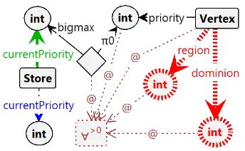
[image:4.595.53.284.257.351.2]Within Groove, we represent a parity game by a simple directed graph, containing a set ofVertex objects. The vertices in the graph represent the vertices of both players in the parity game, and have edges between them if they have an edge between them in the parity game. Each of the vertices have edgespriority andparityto the priority and the parity (player) of the vertex respectively. Visually, we depict this representation as in Figure 2.
Figure 2. Representation of a parity game
4.1.2
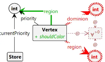
Regions
Based on the graph transformations that take place as a result of actions within the algorithm, we partition the game into regions. We represent this with an optional
region edge from a vertex to a region number. When a vertex does not have such an edge to a region number, it means that it is not in any region.
In addition to regions, the algorithm records dominions to signify that a certain region is won by a certain player. Within the graph, we represent this by having an optional
dominion edge from a vertex to a parity, indicating of which player the dominion is.
4.1.3
Colouring
To make it easier to at a glance distinguish regions, we give every vertex a colour based on the region or dominion it is in. This can help to quickly navigate the states explored by the graph transformations, as the colours prominently display which vertices belong to which region.
Groove provides the functionality to colour vertices. How-ever, these colours are not part of the state, meaning that we have no way to check whether a vertex is already coloured. Hence, we introduce ashouldColor flag, which is set for a vertex whenever its region is changed. Subse-quently, the control program (as described in Section 4.5) takes care of colouring the vertex and removing the should-Color flag. This is simply done by wrapping every graph transformation rule with the potential to update a region in a colour recipe, which first applies the graph transfor-mation and afterwards updates the colour for all vertices where this is necessary. By using a recipe, we ensure that this is displayed to be a single graph transformation, while in reality two graph transformations are applied. As a result, it appears as if the colour is immediately applied whenever the region is updated, and theshouldColor flag never appears in the graph.
4.1.4
Algorithm State
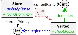
The priority promotion algorithm keeps track of certain variables that record the state of the algorithm. Within the graph, we represent this by having a singleStore ob-ject within the graph, which has edges tocurrentPriority,
currentParity andotherParity that record the current pri-ority, current player and other player within the algorithm respectively.
4.1.5
Finding the Highest Priority
An important basic ingredient of the priority promotion algorithm is finding the highest priority in the remaining subgame. That is, finding the highest priority of any vertex that is not in a region or dominion. We do this using the graph transformation as depicted in Figure 3. Formally, this means that the current priority of the algorithm is updated to equal the priority of vertex u given that u
satisfies the following expression.
notInRegion(u)∧notInDominion(u)∧ ∀v∈vertices
notInRegion(v)∧notInDominion(v)⇒
[image:4.595.338.510.300.406.2]priority(u)≥priority(v)
Figure 3. Set highest remaining priority
[image:4.595.328.518.464.537.2]Whenever the current priority is updated, we must poten-tially update the current parity as well. For this, we use the graph transformation rule as depicted in Figure 4.
Figure 4. Swap players
4.2
Main Loop
4.2.1
Attractor Computation
To compute the attractor of a specific priority, first vertices with that priority that are not in a region or dominion are added to the new attractor. In other words, allu∈vertices
that satisfy the following expression are added to the new attractor.
notInRegion(u)∧notInDominion(u)∧priority(u) =
currentP riority
This leads to the graph transformation rule as depicted in Figure 5. Subsequently, vertices that are not in a region or dominion should be added to the attractor as long as any of the following two conditions is satisfied for the vertex.
1. The vertex has paritycurrentParityand has at least one edge to a vertex in the attractor.
Figure 5. Set region of vertices with current prior-ity
This means that allu∈verticessatisfying one of the fol-lowing two expressions should be attracted to the attractor.
1. parity(u) =currentP arity∧notInRegion(u)∧
notInDominion(u)∧ ∃v∈vertices
edge(u, v)∧
region(v) =currentP riority
2. parity(u) =
otherP arity∧notInRegion(u)∧notInDominion(u)∧ ∃v∈verticesedge(u, v)∧region(v) =
currentP riority
∧ ∀w∈vertices
edge(u, w)∧
notInDominion(w)
⇒inRegion(w)
[image:5.595.309.540.49.138.2]Finally, from these expressions we can construct the graph transformation rules in Figure 6 and Figure 7 respectively. In both these rules, we add astrategy edge from the at-tracted vertex to the vertex causing the attraction, indi-cating the winning strategy of the player at the attracted vertex (given that the region turns out to be a dominion).
Figure 6. Attract vertices of current parity
Figure 7. Attract vertices of other parity
4.2.2
Open and Escapes
After the attractor is fully computed, the open vertices of that attractor must be computed. To find the open vertices, we need to find vertices with paritycurrentParity
that are inside the attractor but have no edges to a vertex inside the attractor. In other words, a vertexu∈vertices
is open whenever the following expression is satisfied.
parity(u) =currentP arity∧region(u) =currentP riority∧ ∀v∈vertices
edge(u, v)⇒region(u)6=region(v)
We indicate that the vertices are open by adding anopen
flag to the vertex. This leads to the graph transformation rule as given in Figure 8.
Figure 8. Find open vertices
To subsequently find the escape vertices, we need to find all successors of vertices with parityotherParity within the attractor that are not in a dominion. In other words, a vertexv ∈ verticesis an escape vertex whenever the following expression is satisfied.
∃u∈vertices[edge(u, v)∧parity(u) =
otherP arity∧region(u) =currentP riority∧region(v)6=
currentP riority∧notInDominion(v)]
We indicate that the vertices are escapes by adding an
[image:5.595.309.541.294.396.2]escape flag to the vertex. From this, we construct the graph transformation rule as given in Figure 9.
Figure 9. Find escape vertices
4.2.3
Detecting Closed Regions
Now that we can find open and escape vertices, we can detect whether a region is closed. For a region to be globally closed, it means that the graph must not contain any open or escape vertices. This means that a region is globally closed once the following expression is satisfied.
∀u∈vertices[notIsOpen(u)∧notIsEscape(u)]
We store the finding that a region is globally closed in the
[image:5.595.55.287.380.600.2]Store object. This leads us to the graph transformation rule as given in Figure 10.
Figure 10. Determine whether attractor is globally closed
If a region is not globally closed, we check for a weaker notion of closedness, namely locally closed. We say that a region is locally closed if the graph does not contain any open vertices, and that all escape vertices are not in the subgame (i.e. have a higher priority region than the current priority). This means that a region is locally closed whenever the following expression is satisfied.
∀u∈vertices[notIsOpen(u)∧isEscape(u)⇒region(u)>
currentP riority]
[image:5.595.318.527.560.595.2]Figure 11. Determine whether attractor is locally closed
4.3
Globally Closed
4.3.1
Reset Other Regions
[image:6.595.310.539.141.199.2]Whenever a region is globally closed, this means that we found a dominion. Because of this, we can reset all other regions (if existing) and delete their strategies, as the algo-rithm needs to be executed again if some vertices are not in a dominion yet. We take care of this by simply removing the region and strategy edges from allu∈verticesthat satisfyregion(u)6=currentP riority, which leads to the graph transformation rule as given in Figure 12.
Figure 12. Reset regions outside attractor
4.3.2
Handling Dominions
After resetting all other regions, the vertices in the par-ity game are either in a dominion, in the attractor or in no region at all. As some vertices not in a region may want or need to move their tokens to the attractor, we compute the attractor once more using the graph transfor-mation described in Section 4.2.1. Afterwards, we return the dominion, indicating that the attractor is won by a certain player. We remove theregionedge and add a do-minion edge to the parity of that player. We do this for allu∈verticessatisfyingregion(u) =currentP riority. In addition, we indicate in theStoreobject that a dominion is found so that the control program knows that we should leave the main loop. This is equivalent to applying the graph transformation rule as given in Figure 13.
Figure 13. Mark attractor as dominion
4.4
Locally Closed
4.4.1
Merge Regions
If a region is not globally closed but is locally closed, it means that there are escape vertices, but only in previously computed regions. We want to merge the attractor into the region of lowest escape, but for this we first need to find the lowest escape region. That is, the region of a vertex
u∈verticessatisfying the following expression.
isEscape(u)∧ ∀v∈vertices
isEscape(v)⇒region(u)≤
region(v)
[image:6.595.99.239.292.388.2]At the same time, we update the current priority to equal the priority of the lowest escape region, as we want to merge the attractor into that region. This leads to the graph transformation rule as given in Figure 14.
Figure 14. Set current priority to lowest escape region
We do, however, need to remember the priority of the attractor that we want to merge into the region. We let the control program take care of this, as we describe in Section 4.5. Given that we know the priority of the attractor, we can now easily merge it into the region by replacing the region of the vertices in the attractor by the current priority. In other words, we do this foru∈vertices
[image:6.595.310.538.321.367.2]satisfyingregion(u) =attractorRegion(see Figure 15).
Figure 15. Promote attractor to lowest escape re-gion
4.4.2
Reset Lower Regions
After a promotion, all lower regions must be reset. That is, we remove the region attribute fromu∈verticessatisfying
region(u)< currentP riority. This gives rise to a graph transformation rule similar to the one described in Section 4.3.1, the only difference being that now the region must be smaller than the current priority (see Figure 16).
Figure 16. Reset regions lower than current prior-ity
4.5
Control Program
Now that we have described all the graph transformations, we need to ensure that they are applied appropriately. For this, we use a control program that controls when graph transformations are applied.
[image:6.595.357.489.487.583.2] [image:6.595.87.250.583.656.2]of using a single graph transformation, now at most three different graph transformation rules need to be used. For this, we use the function as given in Algorithm 2. This function is called by the control program instead of a single graph transformation rule.
trysetCurrentPriorityRegion;
alap do try
attractCurrentParity;
else
attractOtherParity;
end end
Algorithm 2:Attractor computation control function
In this function, first the current priority is assigned to vertices with that priority that are not yet in a region. The
trykeyword indicates that even if this graph transformation rule is not applicable, the function will continue regardless. Afterwards, the function will attract vertices to the region as long as possible (keyword alap). The try and else
keywords indicate that first it is tried to attract a vertex of the current parity, but when this is not possible a vertex of the other parity is attracted. As long as any of the two attracting rules are applicable, the function ensures that vertices are continued to be attracted to the region.
In addition to enforcing the order of graph transformation rule applications, the control program takes care of the following technicalities.
1. Initializing theStoreat the beginning of the algorithm and removing it again at the end of the algorithm. 2. “Cleaning up” the state after an iteration of the
algo-rithm. This entails invoking a graph transformation rule that removesopenandescapeflags from vertices and thelocallyClosed flag from the Store.
3. Updating the current parity and other parity in the Store whenever the current priority is updated by the means of a graph transformation.
4. Keeping track of the attractor region that should be merged into the lowest escape region after the current priority is updated.
4.6
Extended Priority Promotion
4.6.1
Non-Deterministic Attractor Computation
The conversion from the default deterministic attractor computation to the non-deterministic one is quite trivial. To accomplish this, we only need to replace thetry-else
construct in the attraction function (Algorithm 2) by a
choice-or construct (Algorithm 3). The choice and or
keywords indicate that non-deterministically a choice is made between attracting a vertex of the current parity and a vertex of the other parity. In order to do a complete state space exploration and enumerate the different winning strategies, we also need to ensure that the exploration strategy in Groove is set to breadth-first search.
4.6.2
Non-Deterministic Closed Region Handling
We may find a solution faster if we sometimes ignore a closed region. We can model this in Groove by wrapping the part that handles closed regions in achoice-orconstruct (as described in Section 4.6.1), and setting the exploration strategy in Groove to breadth-first search. This causes a non-deterministic choice to be made between the normal behaviour (immediately treating a closed region) and the alternative behaviour (continuing the algorithm without handling it), allowing us to inspect which works better.
trysetCurrentPriorityRegion;
alap do choice
attractCurrentParity;
or
attractOtherParity;
end end
Algorithm 3:Non-deterministic attractor computation control function
4.6.3
Recursive Priority Promotion
[image:7.595.327.521.275.328.2]In order to recursively find a dominion in an attractor, we need to keep track of the current recursion level and remember which vertices are in which recursion level, while data from “higher” levels should not get overwritten. We take care of this by having Store objectsin other Store objects, where every Store object has a level assigned to it. The transformation rule to do this is given in Figure 17.
Figure 17. Initiate recursive call
All vertices in the attractor (that are not open and not attracted to open vertices) also get assigned the level of the “deepest” Store object, indicating that they are a part of the subgame that should be investigated recursively. We then recursively call the function to find a dominion, treating only the vertices with the appropriate level. After finding a dominion, we go back to the supergame by removing the level labels from the vertices and removing the deepest Store object (see Figure 18), while keeping the found do-minion as an attractor. Then we check whether this region is globally or locally closed and treat it accordingly, after which we continue with the algorithm as usual.
Figure 18. Return from recursive call
4.7
Conversion Tool
Another result of the research is a tool to easily convert textual representations of parity games as used by Oink[17] to graph representations in Groove on which the modelled graph transformations can be executed.
5.
CONCLUSION
As explained in Section 4, we have modelled the priority promotion algorithm as a series of graph transformations. In addition, we have extended the algorithm by introduc-ing non-deterministic attractor computations: instead of immediately attracting a vertex whenever we find a pos-sibility to do so, we let Groove do a complete state space exploration for all possible different attractor computations. This allows us to enumerate all different winning strategies produced by different attractor computations, and visu-ally inspect the steps taken to get there. And because of the versatility of Groove, we can easily remove this non-determinism again by setting the state space exploration strategy to linear search.
regions, we can potentially save time, as we can find domin-ions with low priorities earlier. In some of our examples, this turns out to be advantageous (16 total attractions instead of 19). Further research would be required to in-fer a general rule about when the recursive algorithm is better. Moreover, we have extended the algorithm by non-deterministically treating a closed region. Also this turned out to be beneficial in some of our test cases, in particular when ignoring locally closed regions. For further research it might be interesting to investigate in what types of cases delayed promotion or dominion return is advantageous.
Next to modelling the priority promotion algorithm (and extensions thereof), we have developed a tool that allows for easy conversion to Groove parity games, which makes it easier for researchers to use the modelled graph trans-formation rules in practice. In turn, this can increase their understanding of the priority promotion algorithm, and parity game algorithms in general.
One aspect of the research that we could have approached in a different way, is not making use of a control program and instead only using “pure” graph transformations. If we would have done this, we would have needed to keep track of the algorithm state somewhere in the graph (such as in the
Storeobject), as the order of the graph transformations still needed to be enforced. This would have required to verify at every graph transformation rule whether the algorithm was in the correct state to apply the transformation.
We used a control program, because not doing so would mean that both intermediate states and graph transforma-tion rules would become cluttered with informatransforma-tion. This information would not be relevant to the users inspecting the states (as it is mostly internal information specific to the implementation), but would cloud their view of the important information and as a result make the functioning of the algorithm more difficult to understand. In addition, not using a control program would make it impossible to hide trivial graph transformations to the users, such as the updating of the current parity after updating the current priority and the colouring of vertices based on their regions.
It will be interesting to see to what degree the visualisation of priority promotion by the means of graph transforma-tion in Groove increases the general understanding about parity game algorithms. Looking forward, it will also be interesting to investigate how we can model other parity game algorithms using graph transformations, as we can then visually compare their functioning and performance to the priority promotion algorithm, and study their relative practical complexity. In addition, because we have already succeeded in modelling extended versions of the priority promotion algorithm as series of graph transformations, we can attempt to modify certain other aspects of the algorithm and reflect these changes in the graph transfor-mations, in order to investigate in what way the functioning and performance of the algorithm are altered. In the end, we hope that these findings contribute to eventually finding a polynomial solution for solving parity games.
6.
ACKNOWLEDGEMENTS
First of all, I would like to thank my very helpful supervisor Tom van Dijk for supervising my project, and for being very patient with me in helping me grasp the idea of parity game algorithms near the beginning of the project.
In addition, I would like to thank Arend Rensink for allow-ing me to join theSoftware Sciencemaster course about
graph transformations, and for taking the time to evaluate my graph transformations despite his very busy schedule.
Finally, I would like to thank my family and friends for all their moral support and advice.
7.
REFERENCES
[1] A. Beckmann and F. Moller. On the complexity of parity games. InBCS Int. Acad. Conf., pages 237–248. British Computer Society, 2008. [2] M. Benerecetti, D. Dell’Erba, and F. Mogavero.
Improving priority promotion for parity games. In
HVC, volume 10028 ofLNCS, pages 117–133, 2016. [3] M. Benerecetti, D. Dell’Erba, and F. Mogavero. A
delayed promotion policy for parity games.Inf. Comput., 262(Part):221–240, 2018.
[4] M. Benerecetti, D. Dell’Erba, and F. Mogavero. Solving parity games via priority promotion.Formal Methods in System Design, 52(2):193–226, 2018. [5] A. Bohy, V. Bruy`ere, E. Filiot, and J. Raskin.
Synthesis from LTL specifications with mean-payoff objectives. InTACAS, volume 7795 ofLNCS, pages 169–184. Springer, 2013.
[6] J. C. Bradfield and I. Walukiewicz. The mu-calculus and model checking. InHandbook of Model Checking, pages 871–919. Springer, 2018.
[7] W. Czerwinski, L. Daviaud, N. Fijalkow,
M. Jurdzinski, R. Lazic, and P. Parys. Universal trees grow inside separating automata: Quasi-polynomial lower bounds for parity games. InSODA, pages 2333–2349. SIAM, 2019.
[8] E. A. Emerson and C. S. Jutla. Tree automata, mu-calculus and determinacy (extended abstract). In
FOCS, pages 368–377. IEEE Computer Society, 1991. [9] E. A. Emerson, C. S. Jutla, and A. P. Sistla. On
model checking for theµ-calculus and its fragments.
Theor. Comput. Sci., 258(1-2):491–522, 2001. [10] J. Fearnley. Efficient parallel strategy improvement
for parity games. InCAV (2), volume 10427 ofLNCS, pages 137–154. Springer, 2017.
[11] O. Friedmann and M. Lange. Solving parity games in practice. InATVA, volume 5799 ofLNCS, pages 182–196. Springer, 2009.
[12] O. Friedmann and M. Lange. A solver for modal fixpoint logics.ENTCS, 262:99–111, 2010.
[13] M. Jurdzinski. Small progress measures for solving parity games. InSTACS, volume 1770 ofLNCS, pages 290–301. Springer, 2000.
[14] B. K¨onig, D. Nolte, J. Padberg, and A. Rensink. A tutorial on graph transformation. InGraph Transformation, Specifications, and Nets, volume 10800 ofLNCS, pages 83–104. Springer, 2018. [15] F. Mogavero, A. Murano, and L. Sorrentino. On
promptness in parity games. InLPAR, volume 8312 ofLNCS, pages 601–618. Springer, 2013.
[16] T. van Dijk. Attracting tangles to solve parity games. InCAV (2), volume 10982 ofLNCS, pages 198–215. Springer, 2018.
[17] T. van Dijk. Oink: An implementation and
evaluation of modern parity game solvers. InTACAS (1), volume 10805 ofLNCS, pages 291–308. Springer, 2018.