Predicting optimal facility location without customer locations

warwick.ac.uk/lib-publications

Original citation:

Yilmaz, Emre, Elbasi, Sanem and Ferhatosmanoglu, Hakan (2017) Predicting optimal facility

location without customer locations. In: 23rd ACM SIGKDD International Conference on

Knowledge Discovery and Data Mining, Halifax, NS, Canada , 13-17 Aug 2017. Published in:

KDD '17 Proceedings of the 23rd ACM SIGKDD International Conference on Knowledge

Discovery and Data Mining pp. 2121-2130.

Permanent WRAP URL:

http://wrap.warwick.ac.uk/92539

Copyright and reuse:

The Warwick Research Archive Portal (WRAP) makes this work by researchers of the

University of Warwick available open access under the following conditions. Copyright ©

and all moral rights to the version of the paper presented here belong to the individual

author(s) and/or other copyright owners. To the extent reasonable and practicable the

material made available in WRAP has been checked for eligibility before being made

available.

Copies of full items can be used for personal research or study, educational, or not-for profit

purposes without prior permission or charge. Provided that the authors, title and full

bibliographic details are credited, a hyperlink and/or URL is given for the original metadata

page and the content is not changed in any way.

Publisher’s statement:

"© ACM, 2017. This is the author's version of the work. It is posted here by permission of

ACM for your personal use. Not for redistribution. The definitive version was published in

KDD '17 Proceedings of the 23rd ACM SIGKDD International Conference on Knowledge

Discovery and Data Mining.http://doi.acm.org/10.1145/3097983.3098198 "

A note on versions:

The version presented here may differ from the published version or, version of record, if

you wish to cite this item you are advised to consult the publisher’s version. Please see the

‘permanent WRAP URL’ above for details on accessing the published version and note that

access may require a subscription.

Predicting Optimal Facility Location without Customer

Locations

Emre Yilmaz

Computer Engineering Department Bilkent University

Ankara, Turkey [email protected]

Sanem Elbasi

Computer Engineering Department Bilkent University

Ankara, Turkey [email protected]

Hakan Ferhatosmanoglu

Bilkent University Ankara, Turkey [email protected]

ABSTRACT

Deriving meaningful insights from location data helps businesses make be�er decisions. One critical decision made by a business is choosing a location for its new facility. Optimal location queries ask for a location to build a new facility that optimizes an objective function. Most of the existing works on optimal location queries propose solutions to return best location when the set of exist-ing facilities and the set of customers are given. However, most businesses do not know the locations of their customers. In this paper, we introduce a new problem se�ing for optimal location queries by removing the assumption that the customer locations are known. We propose an optimal location predictor which accepts partial information about customer locations and returns a location for the new facility.�e predictor generates synthetic customer locations by using given partial information and it runs optimal location queries with generated location data. Experiments with real data show that the predictor can�nd the optimal location when su�cient information is provided.

CCS CONCEPTS

•Information systems→Data analytics;Uncertainty;•�eory of computation→Facility location and clustering;

KEYWORDS

Location Analytics; Optimal Location�eries; Uncertainty; Predic-tion; Data Generation

1 INTRODUCTION

Location analytics is the process or the ability to gain insight from the location data. Businesses use location analytics in many ways [8] such as�nding the best place to locate a new facility, identifying the performances of stores, analyzing sales in di�erent regions to o�er products and prices most suitable for these regions, and managing insurance risks based on the potential of disasters in given locations. In this work, we consider the problem of selecting the optimal location which is a common location-based analysis that seeks the best location to open a new facility optimizing an objective function given a set of existing facilities and a set of customers.�e objective function may vary depending on the aim of the business. For instance, a business may want to maximize the customers a�racted by the new facility. In that case, the new facility must be the closest facility of as many customers as possible.

KDD’17, August 13–17, 2017, Halifax, NS, Canada.

f1/ 3

f2/ 7

f3/ 6

f5/ 4

f4/ 5

p1 _p2

p3

p4 _{Existing facility}

Candidate location

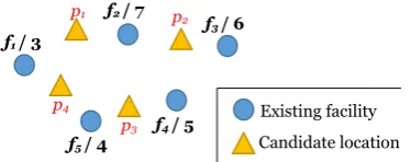
Figure 1: An example scenario for the problem.

Another objective can be minimizing the average distance of the customers to their closest facilities. For instance, delivery services pay a�ention to decreasing the average distance to reduce their logistics costs.

Previous works on optimal location queries focus on returning the best candidate as fast as possible [6, 15, 21]. Some of these works select the optimal location from a given region, whereas the others select from a set of candidate locations.�e common approach is to use pruning based algorithms and index structures to decrease the processing times, instead of sequentially checking each possible location.�e methods in the literature mostly�nd the optimal location when the locations of existing facilities and the locations of customers are given. Hence, businesses need to know the locations of their customers in order to use these algorithms. However, this is rarely the case. Most businesses do not have the knowledge of customer locations. For example, fast food restaurant chains or co�eehouse chains typically do not know the addresses of their customers.�erefore, when these businesses plan to open new branches, they cannot use the existing techniques for�nding the optimal location.

In this paper, we introduce a new se�ing for the optimal location problems: A business that wants to�nd the optimal location for its new facility does not know the location of its customers. Instead, some partial information is known by the business such as the total number of customers a�racted by each existing facility. Although many businesses do not know exact locations of their customers, they naturally have the number of customers for each existing facility. Figure 1 shows an example scenario for the addressed problem, where a business has�ve existing facilities and it has the knowledge of total number of customers a�racted by each facility. For instance, there are 3 customers whose nearest facility isf1in

Figure 1.�e business needs to decide the best location among the candidates to open a new facility.

predicts the optimal location a�er running the query on generated location data. Customer locations are generated based on the to-tal number of customers a�racted by each facility. We form the Voronoi diagram for existing facilities and generate the customers of each facility in its Voronoi region. Instead of just uniformly distributing the customers within each Voronoi region, we use the density of customers in neighbor facilities in Voronoi diagram by dividing the Voronoi region of each facility into triangular regions and generating the customer locations in these smaller regions. It is possible to apply other constraints in the generation of customer lo-cation data such as removing the areas where no one lives (e.g. seas and forests). We performed experiments on real datasets containing Foursquare check-ins in New York City and Tokyo to show how each additional information increases the accuracy of the predictor.

�e key contributions of the paper are summarized as follows:

• We study the optimal location selection problem by

remov-ing the assumption that the customer locations are known to businesses.

• We develop an optimal location predictor for choosing a

location for the new facility by generating customer loca-tions based on the density of the customers in each existing facility and the given auxiliary information.

• Our experiments with real location data from New York

City and Tokyo show that the proposed predictor�nds the optimal location for the new facility among several candidates even though the customer locations are not known.

�e rest of the paper is organized as follows. Related work is re-viewed in Section 2. Section 3 formulates the problem. We explain the optimal location predictor in Section 4 and evaluate the per-formance of the predictor through experiments with real data in Section 5. Finally, Section 6 concludes the paper.

2 RELATED WORK

Nearest neighbor (NN) query is a well-studied problem with many variants in the literature [1, 7, 14]. Reverse nearest neighbor (RNN) query�nds the set of points that have the query point as the nearest neighbor [11]. In most of the real-life applications bichromatic reverse nearest neighbor (BRNN) query is used. In BRNN, points are divided into two categories such as customers and facilities. Given a facilityf, BRNN query�nds the set of customers that have f as the nearest facility. BRNN query is a fundamental query for

optimal location studies because generally it is assumed that each customer prefers her closest facility. Hence, BRNN of a facility is the set of customers who are a�racted by that facility.

Identifying the optimal location for a new facility has been widely studied in the literature with applications in decision-support sys-tems and strategic planning of businesses. An optimal location query asks for a location to build a new facility that optimizes an objective function. For di�erent types of facilities, di�erent objec-tive functions can be used. We consider two di�erent objectives in this work: (i)max-inf:maximizing total number of customers at-tracted by the new facility and (ii)min-dist:minimizing the average distance between each customer and her nearest facility.

Max-inf optimal location query:Given a setF of existing

facilities and a setCof customers, max-inf optimal location query

�nds a locationpfor the new facility with maximum in�uence.

In [6], the in�uence of a location is de�ned as the total weight of its BRNN. Each customer has a weight and the query computes a locationpin a given regionQwhich maximizes the total weight of

customers who are closer topthan to any facility.�e problem is

studied inL1-norm space and the authors propose methods using

di�erent index structures such asR⇤-tree, tree and virtual

OL-tree. Maximizing the BRNN of the new facility inL2-norm space is

studied in [19]. Utilizing the region-to-point transformation, the authors solve the problem by searching a limited number of points instead of searching all possible points in the space. �e same problem is studied assuming that each facility has a given capacity [3]. Another study returns top-klocations from a set of candidate

locations instead of the best one [10].�e general assumption in optimal location queries is that each customer prefers her closest facility. In [22], it is assumed that a customer tends to go to herk

nearest facilities. Hence, a facility a�racts customers if the facility is one of herk nearest facilities. �ey�nd an optimal location

such that se�ing up a new facility a�racts the maximum number of customers.

Min-dist optimal location query:Given a setF of existing

facilities and a setCof customers, min-dist optimal location query

�nds a locationpsuch that the average distance from each customer

to her closest facility is minimized if the new facility is built at loca-tionp.�is query is widely used in real-life applications to improve

the quality of service or reduce the logistics cost by businesses. It is

�rstly de�ned in [21] to select the min-dist optimal location from a given region. Although there are in�nite number of locations in a region, the authors prove that it is possible to limit the number of candidate locations inL1-norm space and the exact result is

in-cluded in�nite number of candidate locations. Qi et al. [15] solve the problem inL2-norm space for the set of candidate locations

and investigate the variant of the problem called min-dist facility replacement problem. Instead of adding a new facility, replacing a facility is aimed in facility replacement problem. Algorithms to solve optimal location queries in road networks have also been studied [4].

Previous works on optimal location queries select the optimal location either from a given region [19, 21] or from a candidate lo-cation set [10, 15]. When it is selected from a given region, in�nite number of candidate locations is�rstly limited.�en it becomes possible to search limited number of candidates. In this work, we select the optimal location from given candidate locations because businesses typically choose the facility locations from several can-didates in practice. In addition, existing works focus on e�ciently returning the best candidate using pruning techniques and index structures. However, they return the optimal location when the exact customer locations are given. Our work di�ers from existing works because we remove the the assumption that the customer locations are known to businesses. We introduce a new problem se�ing in which businesses only know partial information about customer locations.

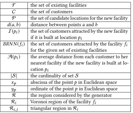
Table 1: Notations used in the paper.

F the set of existing facilities C the set of customers

P the set of candidate locations for the new facility

d₍a,b₎ distance between pointsaandb

I(pi) the set of customers a�racted by the new facility

if it is built at locationpi

BRN N₍f_i) the set of customers a�racted by the facilityf_i

for the given set of existing facilities

A(pi) the average distance from each customer to her

nearest facility if the new facility is built at lo-cationpi

|S| the cardinality of setS

xp abscissa of the pointpin Euclidean space

p ordinate of the pointpin Euclidean space

R the region considered by the generator Ri Voronoi region of the facilityfi

Ri,j triangular region inRi

which the answer of the query depends on both the tuple scores and probabilities. Tao et al. [17] de�ne range queries on uncertain databases to return objects in a given region whose probability is greater than a given threshold, where each object has an imprecise location.�ey propose the concept of probabilistically constrained rectangle and an index structure U-Tree for e�ciently processing uncertain range queries.�e probabilistic nearest neighbor query is�rstly proposed in [5]. In order to return all objects which can be the nearest neighbor of the query point with non-zero probability, their algorithm performs a pruning of objects which do not have a chance of nearest neighbor of the query point. Cheema et al. [2] formalize probabilistic reverse nearest neighbor query that returns the objects which can be the RNN of the query point with higher probability than a given threshold.�ey propose an algorithm using several pruning techniques such as half-space pruning, dominance pruning, metric-based pruning, and probabilistic pruning. Li et al. [12] investigate the problem of probabilistic RkNN query and proposes an e�cient and scalable algorithm using probabilistic pruning and spatial pruning techniques. In all of these works, objects are associated with probabilities and the query results are computed based on these probabilities.�eir approaches cannot be directly applied to our problem because there is no probability associated with customer locations.�e only known information is the number of customers a�racted by each existing facility. Hence, a customer can be located at any point in the Voronoi region of her nearest facility. To the best of our knowledge, our work is the

�rst to address processing of optimal location queries under such uncertainty.

3 PROBLEM FORMULATION

We�rst de�ne max-inf and min-dist optimal location queries and then list the partial and auxiliary information that may be known by businesses to run these queries. Table 1 summarizes the notations used in the paper. All the data objects are represented by points in Euclidean space.

y

y

x

x

Customer whose location is unknown Customer whose location is known

Figure 2: An example scenario for auxiliary information.

D���������1. Given a setF of existing facilities, a setC of

customers, and a setPof candidate locations, themax-inf optimal

location query�nds a locationp2Pfor a new facility such that

8p02P,

|I(p)| I(p0)

whereI(pi)={c|c2C^8f 2F,d(c,pi)d(c,f)}.

D���������2. Given a setF of existing facilities, a setC of

customers, and a setPof candidate locations, themin-dist optimal

location query�nds a locationp2Pfor a new facility such that

8p02P,

A(p)A(p0)

whereA(pi)=

Õ

c2C{d(c,fi) |fi2F[pi^8fj2F[pi,d(c,fi)d(c,fj)}

| C | .

�e above de�nitions of optimal location queries state that the set

Cmust be provided. However, in our problem se�ing, the business

that wants to run optimal location queries does not own the set of customer locations (C). We assume that the business knows

the total number of customers a�racted by each facility. Formally, for each facility f _{2 F},_|BRN N₍f_)|is known by the business

whereBRN N₍f_i) = c_|c_2C^8f_j2F,d₍c,f_i)d₍c,f_j) . To

run optimal location queries, the business can generate a setC0to

mimic_Cbased on the total number of customers a�racted by each facility. However, businesses may have more yet partial information about customer locations. Here, we list auxiliary information (AI) that may be known by businesses and we explain how to use such partial information during the generation of customer locations in Section 4.

AI 1. �e business may know the overallminimum and

maxi-mum valuesfor x and y coordinates in Euclidean space.�ese values

can be represented as follows:

• x_min=min_{x_c|c_2C}

• min=min_{{ c|}c_2C}

• x_max=max_{x_c|c_2C}

• max =max_{{ c|}c_2C}

AI 1 provides the minimum bounding rectangular region for the customer locations. Figure 2 shows an example in which the black and orange points represent customers. AI 1 indicates that all customer data are inside the green rectangle for the example in Figure 2.

AI 2. �e business may know theminimum bounding convex

Data Generator

Optimal Location Query Processor

p ∈P C’

P F

Auxiliary Information

∀ f ∈F, BRNN(f)

Optimal Location Predictor

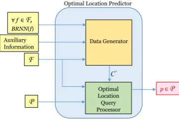
Figure 3: Optimal Location Predictor.

AI 2 provides the convex hull for the customer locations. In Figure 2, the customer locations are bounded with a pentagon drawn with red do�ed lines. Hence, the data generator should generate the all customers inside this polygon if AI 2 is known.

AI 3. �e business may knowempty regionswhich does not

con-tain any customer.

�e business can avoid generating synthetic customer data in regions where no one lives (e.g. seas and forests). For instance, blue circle in Figure 2 represents a lake.�erefore, the data generator should not generate a customer location inside this region.

AI 4. �e business may know asubset ofC.

Although the business does not knowCin the problem se�ing,

locations of some customers may be known. In Figure 2, orange points represent the customers whose locations are known by the business.�erefore, during data generation it is enough to generate the locations for the other customers, who are represented with black points. In Section 4, we present the proposed predictor and ex-plain the usage of auxiliary information during data generation. We also analyze the e�ect of each one on the accuracy of the predictor in Section 5.

4 PREDICTING OPTIMAL LOCATION

In this section, we present our optimal location prediction mecha-nism, when the business knows only|BRN N(f)|for each facility

f 2F.�e business may also know auxiliary information about

customer locations. To run optimal location queries,F,C, and Pmust be given. Since the business does not own the setC, we

propose a location data generator to produce synthetic customer locationsC0that mimicsC.�e query processor then returns the

optimal locationpfor givenF,C0, andP. Figure 3 shows how our

predictor works.

Along with the|BRN N(f)| for each facilityf 2 F, the data

generator needs a regionRfor generating customers in this region.

If the business knows AI 1, the data generator uses the minimum bounding rectangle asR. Otherwise, the business selects a region Rthat will include all synthetic customer locations. To represent Rin�gures clearly, we used a rectangular region. However, it

is not necessary to use a rectangular region. In this region R,

the generator locates the existing facilities (F) and creates the

Figure 4: An example regionRa�er Voronoi Diagram is cre-ated.

Customer whose location is known Existing facility

Figure 5: An example regionRa�er auxiliary information

is considered.

Voronoi diagram which is a partitioning of a plane into convex polygons such that each polygon contains one existing facility

fi 2 F. Voronoi region of each facilityfi 2 F is the set of all

points inRwhose distance tofiis not greater than their distance

to the other facilities. Formally, the Voronoi region of facilityfi 2F

is

Ri = r_{2R |8}f_{j 2F},d₍r,f_i)d₍r,f_j)

An example Voronoi diagram for 5 facilities can be seen in Figure 4. A�er creating the Voronoi diagram, the generator identi�es the regions inRwhich do not contain any customer by checking AI 2

and AI 3. If AI 2 is provided, the generator eliminates the regions in

Rbut not in the minimum bounding polygon during data

genera-tion. If some other empty regions which do not contain a customer (i.e. AI 3) are provided, the generator also eliminates these regions. In Figure 5, these eliminated regions are represented with black. For AI 3, the generator accepts empty regions as polygons. Hence, the business enters the coordinates of the vertices of the polygons for AI 2 and AI 3. In addition, if the business knows a subset ofC

(i.e. AI 4), the locations of these customers are inserted intoR. In

Figure 5, orange points represent the customers whose locations are known by the business.�erefore, they will be included inC0.

A�er considering auxiliary information, the data generator starts generating customer locations for each facilityfi 2F. For a

fa-cilityfi, the generator needs to generate|BRN N(fi)|customers

in its Voronoi regionRi. Ri is a convex polygon and each edge

of the polygon is either a common edge with a neighbor facility or a segment of an edge ofR. It is expected that there are more

customers in the subregions ofRiwhich are close to neighbor

fi

0

0 50

120

30 Ri,1

Ri,2

Ri,3

Ri,4

Ri,5

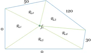
Figure 6: DividingRiinto triangular regions.

regions by connecting each facilityfi 2 F with the vertices of

its Voronoi regionRi. For the given example in Figure 6,Ri is

divided into 5 triangular regions.�e data generator decides the total number of customers to be generated in each triangular region based on:

(1) the area of the region,

(2) the total number of customers a�racted by its neighbor facility.

Let the total number of triangular regions inRi bemi and these

regions be Ri,1, ...,Ri,mi . For a regionRi,j, letBRN N of its

neighbor beni,j. Letni =Õm_k=i₁n_i,k. Hence,niis the total number

of customers a�racted by all of the neighbors off_i.�en, the total

number of customers to be generated in a triangular region_Ri,jis

calculated as

|BRN N(f_i)| ·

✓

·n_ni,j

i +(1 ) ·

Area_(Ri,j)

Area(Ri)

◆

In this formula, is the weighting factor that represents the e�ect ofn_i,jon the total number of customers to be generated inRi,j.

When is selected as 0, the generator distributes customers with respect to the area of each triangle inRi without considering the

number of customers a�racted by neighbors.

For instance, if|BRN N(fi)|is 50 andAr ea_{Ar ea}(R_(Ri_i,3₎)is15 in Figure

6, the generator generates 50·⇣0.5·200120+(1 0.5) ·15 ⌘

=20

cus-tomers inRi,3if is selected as 0.5. For di�erent values of in

the range of[0,1], the total number of customers to be distributed

inRi,3varies between 10 and 30.

By using the given formula, the generator decides the number of customers in each triangular region and produces the customer locations. To produce a random location inside a triangle, one can select three random pointss1,s2,s3in the range of [0,1] such

thats1+s2+s3 = 1 and use these three points as barycentric

coordinates of the random point inside the triangle. For a triangle with verticesP1,P2, andP3, the random point can be determined

ass1·P1+s2·P2+s3·P3.

If the locations of some customers are given as auxiliary infor-mation (i.e. AI 4), the generator generates the locations for the other customers. If some part of the triangular region is removed by AI 2 or AI 3, the area of the remaining region is considered in the formula.

A�er generating synthetic customer locations, optimal location query is executed by the predictor. In max-inf optimal location query, the size of the in�uence set (|I(p_i)|) for each candidate

(a) New York City (b) Tokyo

Figure 7: �e regions covering all customer locations on map.

p_i 2 Pis calculated. �e candidates are ranked with respect to

sizes of their in�uence sets and the candidate with maximum size is returned as the best candidate. In min-dist optimal location query, the average distance (A(p_i)) from each customer to nearest facility

is calculated if the new facility is built at the locationp_i. Similarly,

the candidates are ranked with respect to the average distance values and the candidate with minimum value is returned as the best candidate.

5 EXPERIMENTAL RESULTS

In our experiments, we used datasets [20] containing 227,428

check-ins in New York City and 573,703 check-ins in Tokyo collected from

Foursquare from 12 April 2012 to 16 February 2013. Each check-in in the datasets contains time stamp, GPS coordinates, and venue information. We only used GPS coordinates and we considered each check-in as a separate customer. Hence, there are 227,428

customers inCN YCand 573,703 customers inCT KY. For existing

facilities, we used the locations of 97 McDonald’s restaurants in New York (FN YC) and 76 Yoshinoya restaurants in Tokyo (FT KY).

Figure 7a and 7b show the whole regions containing customer locations on map for New York City and Tokyo, respectively. We divided the whole region into a 10x10 grid for each city and selected the center of each grid as a candidate location for the new facility. We removed the candidates that are in empty regions (e.g. seas). Hence,PN YCandPT KY contain 69 and 72 candidate locations,

respectively.

We implemented our predictor to evaluate its accuracy for max-inf optimal location query and min-dist optimal location query. Initially, we executed these queries using real customer locations (CN YCandCT KY) and we ranked all candidate locations (PN YC

andPT KY) with respect to their optimalities. We determined the

best candidates for max-inf optimal location query and min-dist optimal location query. Letribe the ranking of the candidate

lo-cationpi when real customer location data is used. To observe

the accuracy of the predictor, we counted the total number of cus-tomers a�racted by each existing facility inFN YCandFT KY. We

provided these values (BRN N(f)for each facilityf 2FN YCand

f 2FT KY) to the predictor together with auxiliary information.

�e data generator produced synthetic customer locations (C0N YC

andC0T KY) and we observed the rankings of the candidate

r_i0be the ranking of the candidate locationpi returned from the

predictor. We evaluate the accuracy of the predictor by measuring the standard deviation of the rankings with the following formula:

v

tÕ| P |

i=1(ri ri0)2

|P|

where|P|is the number of candidates. We ran the predictor several

times to show the e�ect of auxiliary information on the accuracy of the predictor. We also ran the predictor with di�erent values to observe the e�ect of on accuracy. We present the evaluation results for max-inf optimal location query and min-dist optimal location query in Section 5.1 and 5.2, respectively. For each query type, we�rstly present the results for =0.5 and then show the

e�ect of on the accuracy.

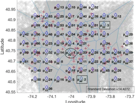
We also illustrate the ranking of the candidates with�gures. In these�gures, the red plus signs represent the existing facili-ties (_{FN YC}and_{FT KY}), the gray circles represent the customers (_{CN YC} and_{CT KY}), the blue diamonds represent candidate loca-tions (_{PN YC}and_{PT KY}), and the blue lines show the boundaries of the Voronoi regions of existing facilities. We marked the best candidates with circles and second best and third best candidates with rectangles. In addition, we show the ranking of the candidates asp_i:j, in whichp_irefers to a candidate location andjrefers to its

ranking.

5.1 Max-Inf Optimal Location

�

ery

Max-inf optimal location query returns a candidate locationpi

which maximizes the total number of customers a�racted by the new facility if it is built at the locationpi. Figure 8 and 9 show the

rankings of the candidate locations inPN YCandPT KY when real

customer locations (CN YCandCT KY) are used.

In New York City, the best candidate for maximizing the total number of customers a�racted by the new facility isp32as shown

in Figure 8. It a�racts 5,341 customers.�e other candidates in top �ve arep46,p30,p47, andp41, and the total number of customers

a�racted by these candidates are 4,599, 3,551, 3,321, and 3,025,

respectively.

In Tokyo, the best candidate returned from max-inf optimal location query isp53and the total number of customers a�racted

by the new facility is 42,411 if it is built at the locationp53.�e other

candidates in top�ve arep32,p9,p46, andp55, and the total number

of customers a�racted by these candidates are 13,528, 13,384, 13,338,

and 10,458, respectively.

In the evaluation of the predictor, we providedBRN N(f)for each

facilityf 2FN YCandf 2FT KY to the predictor. Figure 10 and 11

show the rankings when minimum and maximum coordinates (i.e. AI 1) are also provided to the predictor. For both cities, the predictor returns the same best candidate with the knowledge of AI 1.�e predictor estimates the total number of customers a�racted byp32

as 11,357 in New York City and the total number of customers

a�racted byp53as 33,989 in Tokyo. In New York City, the predictor

also�nds the same second best candidate correctly.�e standard deviations in the rankings for New York City and Tokyo are 14.4272

and 12.9271, respectively.

When we also provide AI 2 and AI 3 to the predictor, it still returns the same best candidates as shown in Figure 12 and 13.

Figure 8: Ranking of candidate locations in NYC when real data is used in max-inf optimal location query.

Figure 9: Ranking of candidate locations in Tokyo when real data is used in max-inf optimal location query.

Moreover, using AI 2 and AI 3 decreases the standard deviation of the rankings. �e standard deviation decreases from 14.4272

to 12.2451 in New York and decreases from 12.9271 to 11.6583 in

Tokyo.�is result indicates that providing more information to the predictor improves the accuracy in the rankings, as expected.

Figure 10: Ranking of candidate locations in NYC when the predictor uses AI 1 in max-inf optimal location query.

Figure 11: Ranking of candidate locations in Tokyo when the predictor uses AI 1 in max-inf optimal location query.

We also conducted experiments to observe the impact of on the standard deviation. As it is mentioned in Section 4, when is equal to 0 the distribution is only based on the areas of the triangles. Hence, we use =0 as the baseline which provides a distribution

in Voronoi region that is similar to uniform distribution. Figure 14b shows the standard deviation for di�erent values of between 0 and 1 when AI 2 and AI 3 are provided to the predictor. For both cities, minimum standard deviation is obtained when is selected as 0.3. �e standard deviation is 11.8248 in New York City and

11.5614 in Tokyo when is equal to 0.3. We also analyzed the

rankings and we observed that the predictor’s top�ve candidates are same for =0.3 and =0.5. As evident in Figure 14b, best

accuracy is achieved when value is in the range of[0.2,0.5].�e

Figure 12: Ranking of candidate locations in NYC when the predictor uses AI 2 and AI 3 in max-inf optimal location query.

Figure 13: Ranking of candidate locations in Tokyo when the predictor uses AI 2 and AI 3 in max-inf optimal location query.

standard deviation is lower than the baseline ( =0) when is

selected in this range.

0 20 40 60 80 100

% of the known customer locations

0 2 4 6 8 10 12

Standard Deviation

New York City Tokyo

(a) Impact of AI 4

0 0.2 0.4 0.6 0.8 1

11.5 12 12.5 13 13.5 14 14.5

Standard Deviation

New York City Tokyo

(b) Impact of

Figure 14: Impact of AI 4 and on the standard deviation of rankings in max-inf optimal location query.

0 20 40 60 80 100

% of expansion of minimum bounding rectangle 12

13 14 15 16 17 18

Standard Deviation

New York City Tokyo

Figure 15: Standard deviation of rankings when no AI is known in max-inf optimal location query.

deviation. However, the predictor returns the same best candidates for both cities without using auxiliary information, because max-inf optimal location query returns the candidate which a�racts maximum amount of customers without considering the distances from customers to their nearest facilities.�erefore, the e�ect of generating customers outside the minimum bounding rectangle on the best candidate is low in max-inf optimal location query.

5.2 Min-Dist Optimal Location

�

ery

Min-dist optimal location query returns a candidate locationpi

which minimizes the average distance between each customer and her nearest facility if the new facility is built at the locationpi. We

conducted the same set of experiments for this query as well. Figure 16 shows the ranking of candidates (PN YC) in NYC when the real

customer locations (CN YC) are used in min-dist optimal location

query. In New York City, the average distance of customers to their nearest facilities are minimized if the new facility is built atp46. �e average distance becomes 1.4433 km ifp46is selected as the

location of the new facility. �e other candidates in top�ve are

p65,p14,p30, andp54, and building a new facility at these locations

decreases the average distances to 1.4567 km, 1.4587 km, 1.4588

km, and 1.4611 km, respectively.

�e ranking of candidates (PT KY) in Tokyo is given in Figure 17

when the real customer locations (CT KY) are used. In Tokyo, the

best candidate for min-dist optimal location query isp3.�e average

distance becomes 1.3346 km, if the new facility is built atp3.�e

other candidates in top�ve arep2,p32,p72, andp53, and building a

Figure 16: Ranking of candidate locations in NYC when real data is used in min-dist optimal location query.

Figure 17: Ranking of candidate locations in Tokyo when real data is used in min-dist optimal location query.

new facility at these locations decreases the average distances to 1.3431 km, 1.3436 km, 1.346 km, and 1.3475 km, respectively.

Table 2 shows the top�ve candidates for both cities according to the predictor with only AI 1. In New York City, the predictor returnsp65as the best candidate, which is actually the second best

candidate as shown in Figure 16.�e real best candidate (p46) is

ranked third by the predictor. In Tokyo, the predictor returnsp72

as the best candidate; however, its actual rank is 5.�e real best candidate (p3) is ranked second by the predictor. �e standard

deviation is 12.7632 in New York City and 12.5266 in Tokyo, when

only AI 1 is provided to the predictor.

Table 2: Top�ve candidate locations when the predictor uses AI 1 in min-dist optimal location query.

New York City Tokyo

Rank Candidate Avg. Dist. Candidate Avg. Dist.

1 p65 1.8667 km p72 1.8319 km

2 p54 1.8667 km p3 1.8354 km

3 p46 1.891 km p64 1.8371 km

4 p55 1.8949 km p4 1.8387 km

5 p32 1.9011 km p52 1.8462 km

Table 3: Top�ve candidate locations when the predictor uses AI 2 and AI 3 in min-dist optimal location query.

New York City Tokyo

Rank Candidate Avg. Dist. Candidate Avg. Dist.

1 p₄₆ 1.6235 km p₃ 1.6487 km

2 p54 1.6265 km p64 1.6549 km

3 p55 1.6286 km p53 1.656 km

4 p37 1.6317 km p2 1.6593 km

5 p28 1.6333 km p4 1.6605 km

�erefore, distance from a customer to her nearest facility is usually higher than the real one, which a�ects the accuracy considerably. AI 2 and AI 3 should be provided to the predictor to achieve a be�er accuracy.

Table 3 shows top�ve candidates according to the predictor, when we provided AI 2 and AI 3 to the predictor. It found the same best candidates for both New York City and Tokyo.�e average distance values are closer to the real values, when the predictor uses AI 2 and AI 3.�e standard deviation also decreases from 12.7632

to 11.0362 in New York and decreases from 12.5266 to 10.1009 in

Tokyo.

Similar to max-inf optimal location query, the standard deviation of the rankings is inversely proportional to the ratio of known customer locations (i.e. AI 4). Standard deviation for di�erent values of percentage of known customer locations is given in Figure 18a. As evident in Figure 18a, the accuracy of the predictor increases when the locations of more customers are provided to the predictor. Figure 18b shows the standard deviation for di�erent values of between 0 and 1 when AI 2 and AI 3 are provided to the predictor in min-dist optimal location query. In New York City, minimum standard deviation (10.3881) is obtained when =0.4. In Tokyo,

standard deviation is minimum (9.9163) when = 0.2. In both

cities, the best accuracy is achieved when value varies between 0.2 and 0.5. Similar to max-inf optimal location query, selecting value in the range of[0.2,0.5]provides be�er accuracy than

the baseline ( =0). Moreover, when we analyze the rankings of

candidate locations, the predictor’s top�ve candidates are same for all values in this range.�erefore, should be selected between 0.2 and 0.5 to improve accuracy.

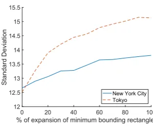
Figure 19 depicts the standard deviation of the rankings when the given region to the predictor is larger than the minimum bound-ing rectangle. As in max-inf optimal location query, the standard deviation increases when the size of the region increases. Unlike

0 20 40 60 80 100

% of the known customer locations 0

2 4 6 8 10 12

Standard Deviation

New York City Tokyo

(a) Impact of AI 4

0 0.2 0.4 0.6 0.8 1 9.5

10 10.5 11 11.5 12 12.5 13

Standard Deviation

New York City Tokyo

(b) Impact of

Figure 18: Impact of AI 4 and on the standard deviation of rankings in min-dist optimal location query.

0 20 40 60 80 100

% of expansion of minimum bounding rectangle

12 12.5 13 13.5 14 14.5 15 15.5

Standard Deviation

New York City Tokyo

Figure 19: Standard deviation of rankings when no AI is known in min-dist optimal location query.

max-inf optimal location query, the predictor does not return the same best candidates when no auxiliary information is provided.

�erefore, providing auxiliary information in min-dist optimal loca-tion query is more important than max-inf optimal localoca-tion query to�nd the same best candidate.

6 CONCLUSION

value used in data generation should be selected between 0.2 and 0.5 to achieve high accuracy.

Since the predictor generates location data randomly, it may not return the best candidate in the following cases:

• if the di�erence of optimality scores of top two candidates

is low.�e optimality score of a candidatepiis calculated

as|I(pi)|in max-inf optimal location query, andA(pi)

in min-dist optimal location query. For instance, in max-inf optimal location query, if the best candidate a�racts 350 customers and the second best candidate a�racts 348 customers, the predictor may not return the real best can-didate.

• if the total number of existing facilities (i.e.|F |) is low. • if the existing facilities have a highly skewed distribution.

In such cases, knowing the locations of some customers by busi-nesses increases the chance of returning the best one.�e experi-ment results show that providing more information improves the accuracy of the predictor.�e proposed predictor facilitates run-ning optimal location queries by businesses without knowing their customers’ locations.

�e proposed approach can be applied to di�erent optimization problems when data is not available. If there is partial informa-tion about data such as the number of items in di�erent clusters, synthetic data can be generated similarly and it can be used in optimization. Hence, generating synthetic data for di�erent opti-mization problems and evaluating their optiopti-mization performance is a potential follow up of this work. Another follow up work is to apply bootstrap methods for data generation and evaluating their accuracy for the case where the locations of some customers are known.�ese methods allow increasing the data size by generating new samples based on the original samples.�erefore, bootstrap methods for spatial data [9, 13] can also be potentially used for data generation if a subset of customer locations (i.e. AI 4) is known.

ACKNOWLEDGMENTS

Hakan Ferhatosmanoglu was supported in part by the Alexander von Humboldt Foundation.

REFERENCES

[1] Christian B¨ohm and Florian Krebs. 2004.�e k-nearest neighbour join: Turbo charging the KDD process. Knowledge and Information Systems6, 6 (2004), 728–749.

[2] Muhammad Aamir Cheema, Xuemin Lin, Wei Wang, Wenjie Zhang, and Jian Pei. 2010. Probabilistic reverse nearest neighbor queries on uncertain data.IEEE Transactions on Knowledge and Data Engineering22, 4 (2010), 550–564. [3] Fangshu Chen, Huaizhong Lin, Yunjun Gao, and Dongming Lu. 2016. Capacity

constrained maximizing bichromatic reverse nearest neighbor search.Expert Systems with Applications43 (2016), 93–108.

[4] Zitong Chen, Yubao Liu, Raymond Chi-Wing Wong, Jiamin Xiong, Ganglin Mai, and Cheng Long. 2014. E�cient algorithms for optimal location queries in road networks. InProceedings of the 2014 ACM SIGMOD international conference on Management of data. ACM, 123–134.

[5] Reynold Cheng, Dmitri V Kalashnikov, and Sunil Prabhakar. 2003. Evaluating probabilistic queries over imprecise data. InProceedings of the 2003 ACM SIGMOD international conference on Management of data. ACM, 551–562.

[6] Yang Du, Donghui Zhang, and Tian Xia. 2005.�e optimal-location query. In

Advances in Spatial and Temporal Databases. Springer, 163–180.

[7] Hakan Ferhatosmanoglu, Ioanna Stanoi, Divyakant Agrawal, and Amr El Abbadi. 2001. Constrained nearest neighbor queries. InInternational Symposium on Spatial and Temporal Databases. Springer, 257–276.

[8] Lee Garber. 2013. Analytics goes on location with new approaches.Computer

46, 4 (2013), 14–17.

[9] Pilar Garc´ıa-Soid´an, Raquel Menezes, and ´Oscar Rubi˜nos. 2014. Bootstrap ap-proaches for spatial data.Stochastic environmental research and risk assessment

28, 5 (2014), 1207–1219.

[10] Jin Huang, Zeyi Wen, Jianzhong Qi, Rui Zhang, Jian Chen, and Zhen He. 2011. Top-k most in�uential locations selection. InProceedings of the 20th ACM interna-tional conference on Information and knowledge management. ACM, 2377–2380. [11] Flip Korn and S Muthukrishnan. 2000. In�uence sets based on reverse nearest

neighbor queries. InACM SIGMOD Record, Vol. 29. ACM, 201–212.

[12] Jiajia Li, Botao Wang, and Guoren Wang. 2013. E�cient probabilistic reverse k-nearest neighbors query processing on uncertain data. InInternational Conference on Database Systems for Advanced Applications. Springer, 456–471.

[13] Ji Meng Loh. 2008. A valid and fast spatial bootstrap for correlation functions.

�e Astrophysical Journal681, 1 (2008), 726.

[14] Dimitris Papadias, Qiongmao Shen, Yufei Tao, and Kyriakos Mouratidis. 2004. Group nearest neighbor queries. InData Engineering, 2004. Proceedings. 20th International Conference on. IEEE, 301–312.

[15] Jianzhong Qi, Rui Zhang, Yanqiu Wang, Andy Yuan Xue, Ge Yu, and Lars Kulik. 2014.�e min-dist location selection and facility replacement queries.World Wide Web17, 6 (2014), 1261–1293.

[16] Mohamed A Soliman, Ihab F Ilyas, and Kevin Chen-Chuan Chang. 2007. Top-k query processing in uncertain databases. InData Engineering, 2007. ICDE 2007. IEEE 23rd International Conference on. IEEE, 896–905.

[17] Yufei Tao, Xiaokui Xiao, and Reynold Cheng. 2007. Range search on multidi-mensional uncertain data.ACM Transactions on Database Systems (TODS)32, 3 (2007), 15.

[18] Yijie Wang, Xiaoyong Li, Xiaoling Li, and Yuan Wang. 2013. A survey of queries over uncertain data.Knowledge and information systems37, 3 (2013), 485–530. [19] Raymond Chi-Wing Wong, M Tamer ¨Ozsu, Philip S Yu, Ada Wai-Chee Fu, and

Lian Liu. 2009. E�cient method for maximizing bichromatic reverse nearest neighbor.Proceedings of the VLDB Endowment2, 1 (2009), 1126–1137. [20] Dingqi Yang, Daqing Zhang, Vincent W Zheng, and Zhiyong Yu. 2015. Modeling

user activity preference by leveraging user spatial temporal characteristics in LBSNs.IEEE Transactions on Systems, Man, and Cybernetics: Systems45, 1 (2015), 129–142.

[21] Donghui Zhang, Yang Du, Tian Xia, and Yufei Tao. 2006. Progressive computation of the min-dist optimal-location query. InProceedings of the 32nd international conference on Very large data bases. VLDB Endowment, 643–654.