Learning based forensic techniques for source camera identification

(1)

warwick.ac.uk/lib-publications

A Thesis Submitted for the Degree of PhD at the University of Warwick

Permanent WRAP URL:

http://wrap.warwick.ac.uk/86799

Copyright and reuse:

This thesis is made available online and is protected by original copyright.

Please scroll down to view the document itself.

Please refer to the repository record for this item for information to help you to cite it.

Our policy information is available from the repository home page.

(2)

Learning based Forensic Techniques for

Source Camera Identification

by

Ruizhe Li

Thesis

Submitted to the University of Warwick

for the degree of

Doctor of Philosophy

Computer Science

(3)

Acknowledgments

First and foremost I would like to express my deepest sense of gratitude to my

supervisor Prof. Chang-Tsun Li, who has been constantly supportive and inspiring

during my PhD study. His great personality, unlimited patience and tolerance has

educated me a lot more than scientific research.

I wish to express my sincere thankfulness to my annual progress panel

mem-bers Dr. Victor Sanchez, Dr. Arshad Jhumka and Prof. Yongjian Hu for their

guidance and valuable suggestions on my research.

I would also like to thank the colleagues at the University of Warwick, Dr.

Yu guan, Dr. Xingjie Wei, Dr. Yi Yao, Mr. Ning Jia, Mr. Xin Guan, Mr. Alaa

Khadidos, Mr. Xufeng Lin, Mr. Qiang Zhang, Mr. Roberto Leyvac, Mr. Shan Lin

and Mr. Ching-Chun Chang for their kindness not just inside the lab.

I would like to express my deepest gratitude to my parents, Mr. Dongyang

Li and Ms. Xin Ji for their love, understanding and encouragement throughout my

life, which give me the strength to chase whatever I want. To my wife, Ms Lin Lin

for being my side, and all the inspirations and love she brings to my life.

Last but not least, to my friends, Mr. Yile Liu, Ms. Simin Tian, Mr. Boyang

(7)

Declarations

I hereby declare that this dissertation entitled Learning based forensic techniques

for source camera identification is an original work and has not been submitted for

(8)

Abstract

In recent years, multimedia forensics has received rapidly growing attention.

One challenging problem of multimedia forensics is source camera identification, the

goal of which is to identify the source of a multimedia object, such as digital image

and video. Sensor pattern noises, produced by imaging sensors, have been proved

to be an effective way for source camera identification. Precisely speaking, the

conventional SPN-based source camera identification has two application models:

verification and identification. In the past decade, significant progress has been

achieved in the tasks of SPN-based source camera verification and identification.

However, there are still many cases requiring solutions beyond the capabilities of

the current methods. In this thesis, we considered and addressed two commonly

seen but less studied problems.

The first problem is the source camera verification with reference SPNs

cor-rupted by scene details. The most significant limitation of using SPN for source

camera identification is that SPN can be seriously contaminated by scene details.

Most existing methods consider the contaminations from scene details only occur

in query images but not in reference images. To address this issue, we propose a

measurement based on the combination of local image entropy and brightness so as

to evaluate the quality of SPN contained by different image blocks. Based on this

measurement, a context adaptive reference SPN estimator is proposed to address

the problem that reference images are contaminated by scene details.

The second problem that we considered relates to the high computational

complexity of using SPN in source camera identification, which is caused by the

(9)

degrading accuracy, we propose an effective feature extraction algorithm based on

the concept of PCA denoising to extract a small set of components from the

orig-inal noise residual, which tends to carry most of the information of the true SPN

signal. To further improve the performance of this framework, two enhancement

methods are introduced. The first enhancement method is proposed to take the

advantage of the label information of the reference images so as to better

sepa-rate different classes and further reduce the dimensionality. Secondly, we propose

an extension based on Candid Covariance-free Incremental PCA to incrementally

update the feature extractor according to the received images so that there is no

need to re-conduct training every time when a new image is added to the database.

Moreover, an ensemble method based on the random subspace method and majority

voting is proposed in the context of source camera identification to tackle the

perfor-mance degradation of PCA-based feature extraction method due to the corruption

by unwanted interferences in the training set.

The proposed algorithms are evaluated on the challenging Dresden image

(10)

Abbreviations

BM3D Block-matching and 3D filtering

CAI Context adaptive interpolation

CCD Charge-coupled devices

CCIPCA Candid covariance-free incremental PCA

CCN Correlation over circular correlation norm

CFA Color filter array

CLT Central limit theorem

CMOS Complementary-metal-oxide semiconductor

DCT Discrete cosine transform

DFT Discrete Fourier transform

EXIF Exchangeable image file

FFT Fast Fourier transform

FPN Fixed pattern noise

(11)

JEET Junction field-effect transistor

JL Johnson-Lindenstrauss lemma

LDA Linear discriminant analysis

MAP Maximum A-Posteriori probability

MLE Maximum-likelihood estimation

MvDA Multi-view discriminant analysis

PCA Principal component analysis

PCAFE PCA-based feature extraction

PCAI Predictor based on the context adaptive interpolation

PCE Peak-to-correlation energy

PDF Probability density function

PRNU Photo-response non-uniformity noise

RSM Random subspace method

ROC Receiver operating characteristic

SCI Source camera identification

SCV Source camera verification

SPN Sensor pattern noise

TPR True positive rate

ULDA Uncorrelated linear discriminant analysis

(12)

List of Tables

1.1 Thesis chapters and the corresponding publications. . . 15

2.1 Two typical contamination cases . . . 39

3.1 Cameras involved in the experiments. . . 56 3.2 The TPR of different methods with respect to different settings ofS. 57

3.3 The TPR of different methods with respect to different number of

reference images on different image sizes. . . 63

4.1 36 Cameras involved in our experiments . . . 79

4.2 The setup of two SCI scenarios . . . 79

4.3 The dimensionality d of PCA-SPNs obtained from different SPN methods w.r.t. different setting ofT and different reference types. . 81

4.4 TPR (%) of different features with different number of flatfield

refer-ence images. . . 87 4.5 Computational cost (Seconds) of SPN Digest-20% and different types

of features produced by BM3D. . . 89

4.6 The size (MB) of data required to be loaded for SPN Digest-20% and different types of features produced by BM3D. . . 89

5.1 Dimensionality of PCA-SPN with respect to the number of cameras involved in training process on image blocks with size of 512×512

pixels. . . 95

5.2 Cameras from Dresden Image Database. . . 102 5.3 Computational cost of different methods on updating a single camera

to a database. . . 106

(13)

List of Figures

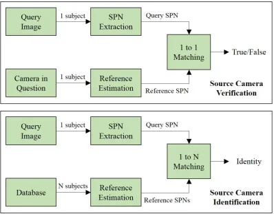
1.1 The flowcharts of source camera verification and identification system. 6 1.2 Examples of the extracted SPN from different images. . . 8

2.1 A simplified depiction of an imaging pipeline within a digital camera. 17 2.2 Examples of the SPNs extracted by using different methods. . . 28

2.3 An example of the enhanced SPN. . . 30

3.1 Intra-class and inter-class PDFs of NCC value calculated from SPNs extracted from different kinds of images. . . 46

3.2 Examples of the varying SPN quality within the images with scene

details. . . 48 3.3 The SPN quality of different image regions within the images with

scene details. . . 52

3.4 The overall ROC curves of difference methods with 15 reference im-ages based on imim-ages with size of 256×256 pixels. . . 58

3.5 The overall ROC curves of difference methods with 30 reference

im-ages based on imim-ages with size of 256×256 pixels. . . 59 3.6 The overall ROC curves of difference methods with 15 reference

im-ages based on imim-ages with size of 512×512 pixels. . . 60

3.7 The overall ROC curves of difference methods with 30 reference im-ages based on imim-ages with size of 512×512 pixels. . . 61

4.1 An example of the reconstrcuted SPN. . . 74 4.2 The TPR (%) of the PCA-SPN obtained from BM3D w.r.t. different

setting of parameterT and different reference types. . . 80

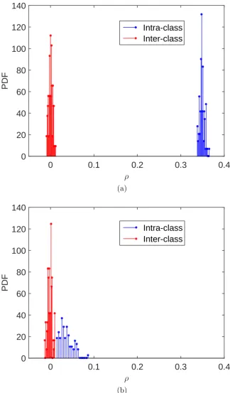
4.3 Distributions of the inter/intra-class correlations w.r.t. different fea-tures and different reference types. . . 83

4.4 Overall ROC curves comparisons among different types of features

(14)

4.5 Overall ROC curves comparisons among different types of features

for the flatfield reference. . . 86

5.1 Distribution of the intra-class and inter-class correlation values ob-tained from the camera not involved in traning. . . 93

5.2 Histograms of the NCC values calculated from features extracted us-ing different methods. . . 103

5.3 The ROC curves of different features based on MLE. . . 105

5.4 The ROC curves of different features based on PCAI8. . . 105

6.1 The flowchart of the RSM-based SCI system. . . 110

6.2 Performance with respect to the number of random subspacesL. . . 118

6.3 Performance with respect to the dimension of the random subspacem.118 6.4 The ROC curves of different methods on image blocks with size of 128×128 pixels. . . 121

6.5 The ROC curves of different methods on image blocks with size of 256×256 pixels. . . 122

(15)

Chapter 1

Introduction

1.1 Background

Nowadays, digital imaging devices, such as digital cameras, camcorders and cameras

embedded in smart phones, are widely used in the modern world. In 2014, more than

1 billion imaging devices have been produced and sold. As a consequence, over one

trillion digital images were taken in that year. With such enormous amount of

digi-tal images, the use of digidigi-tal images as critical evidences in the fight against crime is

increasing, making multimedia forensic investigations more frequent and important.

Typically, multimedia forensics includes source device identification, source-oriented

images classification, integrity verification or forgery detection, authentication, etc.

Source camera identification is a very important branch of multimedia forensics,

which aims to prove whether a given image or video was taken by a specific imaging

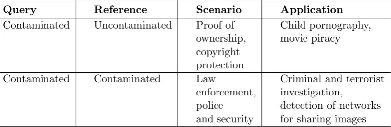
device. This technique has been utilized to identify the origin of digital images or

videos in many forensic cases, such as child pornography, movie piracy, proof of

(16)

abuse case [1], a person was accused of taking a set of child pornography images,

while this suspect refused to plea guilty and claimed that these child pornography

images in his smart phones were downloaded from internet and not taken by him.

The police applied a source camera identification technique and proved that these

images were indeed taken by the suspect’s smart phone. The suspect was finally

convicted after a short trial.

1.2 Source Camera Identification

In order to trace the source of digital images or videos, many efforts have been

made in the task of source camera identification. These proposed techniques can be

roughly divided into three categories:

• Metadata. The simplest technique for identifying the source camera is to use

the metadata embedded by the source camera [2]. For example, exchangeable image

file (EXIF) [3] is a format for storing metadata in image and audio files. The EXIF

header contains information of camera manufacturer, camera model and conditions

under which the image was taken (exposure, date, time, etc.). The EXIF header is

encoded in ASCII text, it can be directly read in the binary file or easily extracted by

using many common photography tools, such as Adobe Photoshop and IrfanView.

One can use this metadata to identify the model of the source camera (but not

the specific camera). However, along with the wide use of these photography tools,

header data can easily be changed or removed by users. In addition, metadata

may not be available if the image is re-saved in a different format or re-compressed.

For these reasons, metadata is not expected to be a reliable indicator of the image

(17)

• Watermarking. Another possible solution to the source camera identification

problem is to use the digital watermark embedded in the image by the camera,

which carries information about the source camera, the time when the image was

taken, and even a biometric data of the person taking the image. There are a

few camera manufacturers offering cameras with watermarking capabilities, which

is called “Secure Camera”, such as Epson PhotoPC 700/750Z, 800/800Z, 3000Z and

Kodak DC-200, DC-260, DC-290 [4]. Such cameras transparently insert a digital

watermark to each image or video they capture, thus one can determine whether a

given image is taken by a specific secure camera by matching the watermark from

the given image and the specific secure camera. This technique is very useful for

proving ownership of a copyright work in the case with secure cameras, while it is

of no help in tracking the source when images are taken by other cameras.

• Manufacturer Specific Technique. The third set of techniques relies on the

intrinsic characteristics of digital cameras left in the image. Generally speaking,

any traces left in the image by the processing components of the image acquisition

pipeline have the potential to link the images to the source camera, such as

sen-sor pattern noise (SPN) [5–14], lens aberration [15, 16], colour filter array (CFA)

interpolation artifacts [17, 18], JPEG compression [2, 19], and the combination of

several intrinsic characteristics [20, 21]. Among these traces, SPN has been proved

as the most effective way for source camera identification, and has attracted the

most attention in the research area. Compared with other intrinsic characteristics,

SPN has several remarkable advantages:

1. Uniqueness. Every image or video taken by the same sensor exhibits the

(18)

SPN patterns even when they are from the same silicon wafer [6].

2. Generality. SPN is present in every digital image and video that captured

by imaging sensors, regardless of the camera optics, settings, or the scene

content [22].

3. Universality. All digital imaging sensors would exhibit SPN pattern, such

as charge-coupled devices (CCD) sensor [23, 24], complementary-metal-oxide

semiconductor (CMOS) sensor [25], junction field-effect transistor (JFET)

sen-sor and CMOS-Foveon X3 sensen-sor [6].

4. Stability. SPN is stable in time and under a wide range of physical conditions,

such as ambient temperature or humidity [22].

5. Robustness. SPN can survive from a series of operations performed on the

image such as blurring, scaling, compression, and even printing and scanning.

Moreover, it is often beyond the capability of normal camera users to

manip-ulate or remove this fingerprint from digital images or videos.

Due to these advantages, the SPN-based sensor fingerprint is quite popular in several

digital forensic applications, such as source camera identification, image clustering,

forgery detection, etc. In this thesis, our research interest is particularly focused on

(19)

1.3 SPN-based Source Camera Verification and

Identi-fication

Precisely speaking, the conventional SPN-based source camera identification has

two application models: verification and identification. Source Camera Verification

(SCV) is the task that conducts one-to-one comparison to verify whether a given

image or video is taken by a specific imaging device. It is especially useful in the

court of law for addressing the question: Is this image taken by the claimed camera?

In order to verify that a query image was taken by a camera, we first need to extract

the SPN from the query image and estimate the reference SPN for the camera. Then

the similarity between the query SPN and reference SPN is calculated. The decision

is finally made by comparing the obtained similarity score with a predetermined

threshold.

On the other hand, source camera identification (SCI) is the task that

search-es a database for an enrolled camera or SPN fingerprint to match the query image,

i.e., one-to-many comparison. The goal of SCI is to answer the question: Which

camera in a database has taken the query image? Different from verification, the

identification system conducts multiple one-to-one comparisons between the query

SPN and a lot of reference SPNs from the database, and returns a single match

(the best match) as the most probable association with the query sample. Fig 1.1

shows the flowcharts of the SPN-based source camera verification and identification.

As illustrated in Fig. 1.1, both the verification and identification system consist of

three main stages: SPN extraction, reference SPN estimation and SPN matching,

(20)

[image:20.595.122.521.106.417.2]

Figure 1.1: The flowcharts of source camera verification and identification system.

1.4 Challenges

The SPN-based source camera identification has been studied for more than a decade

by the multimedia forensic community. Many existing SPN-based methods in the

literature can accurately link digital images or videos to the specific cameras that

acquired them. However, there are still many cases requiring solutions beyond the

capabilities of the current methods. In this thesis, we select the following two

existing problems as the research topic since they are both commonly seen and less

(21)

1.4.1 Reference Images Corrupted by Scene Details

In real-world applications, SPN can be easily contaminated by many interferences,

which would decrease the identification accuracy. Those interference factors can be

roughly summarised into two categories. On the one hand, SPN can be affected by

the characteristics produced in the imaging acquisition process, such as shot noise,

read-out noise, quantization noise, CFA interpolation artifacts, etc [6]. Most

middle-end and high-middle-end cameras have the capability to suppress these contaminations, thus

the impact of these contaminations is relatively low for the identification result,

especially in the uncompressed high quality images. However, it is difficult to fully

remove these contaminations.

On the other hand, SPNs can be contaminated by image content, i.e., scene

edges and textures. As mentioned in [9], both SPN and scene textures appear as

the high-frequency signal, thus in the SPN extraction stage not only the true SPN

components but also the trace of scene textures would be extracted. The interference

of scene textures can be very serious as its magnitude is usually far greater than

that of the true SPN signal in the noise residual [9]. Moreover, it is very common

in real-world environments as most normal images would contain a certain amount

of scene textures. But this contamination can be easily avoided. For example, if

we have access to the camera to be identified, we can use it to take some images of

smooth scenes, such as blue sky and flat wall. By doing so, we can actively avoid

the acquired images from contaminations of scene textures and consequently extract

some clean SPNs. Examples of SPNs extracted from different kinds of images are

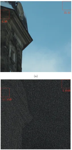
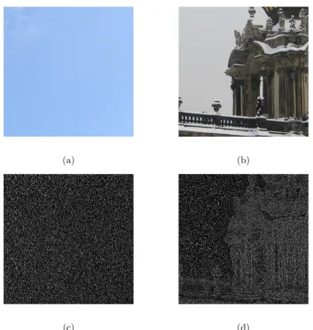
shown in Fig. 1.2. Fig. 1.2 (a) and (b) are a blue sky image and an image with

(22)

(a) (b)

[image:22.595.144.498.109.482.2]

(c) (d)

Figure 1.2: (a) A blue sky image. (b) An image with strong scene details. (c) The SPN extracted from the image (a). (d) The SPN extracted from the image (b). Note the intensity of (c) and (d) has been down scaled 3 times for visualization purpose.

are the SPNs extracted from Fig. 1.2 (a) and (b) by using the method proposed

in [6], receptively. Compared to Fig. 1.2 (b), Fig. 1.2 (a) has much fewer scene

textures so that its corresponding SPN (Fig. 1.2 (c)) is much less contaminated by

scene textures. Therefore, images with smooth regions help to obtain better SPNs.

However, in real-world environments, we may face the problem that the camera

to be identified is absent. For example, a person is suspected of taking images

(23)

already abandoned or hidden his/her camera. Under this circumstance, there is no

smooth images available for the police to estimate a clean reference SPN for the

missing camera. But it is highly conceivable that the images from the suspect’s

Facebook or Flickr accounts are probably taken by the missing camera so that the

police can estimate an SPN from such images to represent the missing camera. If

any SPNs from the images with illegal content are found to be matched with this

estimated SPN, the police can convict this suspect guilty. However, the images from

Facebook or Flickr are very likely to be natural images with varying scene details.

As a result, the SPN extracted from such images might be severely contaminated,

which might lead to a false matching result. Therefore, a challenging problem is

that: is it possible to estimate a trustworthy SPN from images with varying scene

details so as to represent the missing camera?

1.4.2 Source Camera Identification in Large Database

Another challenging problem relates to the high computational complexity of a

SPN-based SCI systems. This problem occurs due to the high dimensionality and

random nature of the SPN fingerprints. Here we provide an example to explain

this problem. A person is apprehended for suspiciously taking pictures of children

near an elementary school, while he/she claims he/she is an amateur photographer

pursuing a hobby. The police plans to estimate a reference SPN for his/her camera

and search a large database of known child pornography images to check whether

any existing clusters in this database match with this reference SPN. Ideally, this

problem can be solved by matching this estimated SPN against all the SPNs of

(24)

whole database. Considering the fact that most images today have more than 106

pixels and there can be tens of thousands of SPN fingerprints in the database, thus

making the computational complexity of a direct search prohibitively high. In this

case, the challenging part is that is it possible to solve this problem more efficiently?

Although the SPN-based technique has been well studied by the research community,

relatively fewer works are devoted to address this problem. Thus, research into the

task of performing source camera identification more efficiently is very important

and necessary.

1.5 Objectives of Thesis

In the view of the above-mentioned challenges, in this thesis, we explore the

fol-lowing two scenarios. The first scenario is effective source camera verification with

reference images corrupted by scene details. As mentioned above, the reference

SP-N estimation is one of main stages in the framework of SPSP-N-based source device

identification. Although there have been several studies dedicated to improving the

performance of SPN based source camera identification, an efficient method for

esti-mating the reference SPN from images with scene details is still lacking. In order to

address this problem, we propose a novel approach for estimating reliable reference

SPN from natural images so as to improve the performance of source camera

veri-fication. In addition, we consider the situation that the number of reference images

taken by the same camera is inadequate (N <50), which is a case most of the

cur-rent works do not take into account. Experimental results show that this method

achieves better performance than the schemes based on the averaged reference SPN,

(25)

The second scenario is efficient source device identification in large database.

Apart from identification accuracy, efficiency is also an important aspect of a source

device identification system, especially when a sizeable database is involved.

Intu-itively, there are two ways to reduce the computational complexity. The first one

is to organize and index the large database into a search tree so that there would

a smaller number of SPN matching to be done. Another one is to find a compact

representation of normal sized SPN so that even a linear search over the whole

database can be performed. In the literature, some efforts have been made in these

two directions. However, while many methods have improved the efficiency, they

undesirably decrease the identification accuracy at the meantime. In the light of

this limitation, we aim at improving the computational efficiency of source camera

identification without degrading the identification accuracy. We employ the concept

of PCA denoising [26–28] in the task of SPN-based source camera identification. An

effective feature extraction algorithm based on this concept is proposed to extract a

small set of components from the noisy SPN, which tends to carry most information

of the true SPN signal. In order to extract components that better represent the

true SPN signal rather than other noises, a training set construction procedure is

proposed to facilitate a more accurate estimation of the feature extractor. In order

to further improve the performance of this framework, two enhancement methods

are introduced. Given the fact that investigators normally have the class label of

the reference images in database, the first enhancement method is proposed to take

the advantage of the label information of the reference images to better separate

different classes and further reduce the dimensionality. Secondly, in real-world

(26)

case, it is infeasible to re-conduct training every time when a new image arrives. To

overcome this limitation, we propose an extension based on Candid Covariance-free

Incremental PCA (CCIPCA) to incrementally update the feature extractor

accord-ing to the received images.

However, the performance of the PCA-based feature extraction method

de-grades when there are some unwanted interferences contained by the training set,

such as the artifacts introduced by scene details, CFA interpolation and JPECG

compression. It is because the eigenvectors that generated from the training process

can be corrupted by these interferences. Some leading eigenvectors are very likely

to represent the interfering components rather than the true SPN signal.

More-over, it is difficult to locate or remove the corrupted eigenvectors from the feature

space. Accordingly, it is difficult to train a reliable feature extractor by using a

noisy training set. To address this problem, we propose a camera identification

framework based on the random subspace method and majority voting. The

ex-perimental results show that this proposed solution is able to suppress the impact

of unwanted interferences, consequently enhancing the identification accuracy. The

main contributionsare summarised in details as follows:

1. We propose a measurement based on the smoothness and brightness to evaluate

the quality of each SPN block for the reference SPN estimation. Based on this

measurement, a reference SPN estimator is proposed to address the problem

that the reference images are contaminated by the scene details [29]. Instead

of treating each SPN block equally for the reference SPN estimation, we weight

each SPN block according to its quality. We also consider the situation that the

(27)

a case most of the current works do not take into account.

2. We employ the concept of PCA denoising in the task of source camera

identifica-tion. A PCA-based feature extraction (PCAFE) algorithm is proposed to address

the issue of prohibitively computational complexity caused by the high

dimen-sionality of SPN [30, 31]. In order to extract components that better represent

the true SPN signal rather than other noises, a training set construction method

is also proposed to minimize the impact of the interfering artifacts in the training

set. In addition, we proposed an extension based on the discriminate analysis

method to take the advantage of the label information of the reference images,

so as to better separate different classes and further reduce the dimensionality.

3. We propose a method based on CCIPCA [32] for incrementally updating the

eigenvectors of the PCA-based feature extractor according to the new received

images. It is an extension of the aforementioned PCAFE method, which is used

to address the costly computation of re-conducting training caused by PCAFE

whenever a new image arrives.

4. We point out the performance of PCAFE decreases when the training set is noisy

and less representative. To address this problem, we propose an ensemble solution

based on the random subspace method (RSM) [33] for the SPN-based source

camera identification. This method can improve the identification accuracy by

combining a large number of weak identifiers in the decision level (i.e., by using

(28)

1.6 Thesis Outline

Chapter 1 provides a brief review of varying techniques used for source camera

identification, which can be roughly divided into three categories: metadata, digital

watermarking and the intrinsic characteristics of digital cameras. Among these

techniques, the advantages of using SPN to solve the source camera identification are

briefly described. This background knowledge is important for further discussions

in this thesis. The next chapter depicts the three main stages of the SCV and

SCI system, and summarizes the related works which have been devoted in them.

Chapter 3 through to 6, the main contributions to the field are elaborated. These

include reducing the impact of scene details in reference SPN estimation (Chapter

3), representing SPN in a compact manner (Chapter 4), feature extractor with

incremental update capability for fast source camera identification (Chapter 5) and

the random subspace method in source camera identification (Chapter 6). Chapter

7 summarises the achievements of this thesis and presents some future research

directions.

1.7 List of Publications

We provide the publication list for my PhD research on SPN-based source camera

identification as follows:

1. R. Li, and C.-T. Li, Y. Guan, “Incremental Updating Feature Extraction for

Camera Identification”, in Proc. IEEE International Conference on Image

(29)

[image:29.595.121.520.138.232.2]

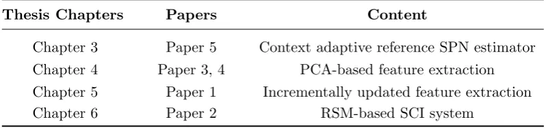
Table 1.1: Thesis chapters and the corresponding publications.

Thesis Chapters Papers Content

Chapter 3 Paper 5 Context adaptive reference SPN estimator Chapter 4 Paper 3, 4 PCA-based feature extraction

Chapter 5 Paper 1 Incrementally updated feature extraction Chapter 6 Paper 2 RSM-based SCI system

2. R. Li, C. Kotropoulos, C.-T. Li, and Y. Guan, “Random Subspace Method

for Source Camera Identification”, in Proc. IEEE International Workshop on

Machine Learning for Signal Processing, Boston, USA, Sept. 17-20, 2015.

3. R. Li, and C.-T. Li, Y. Guan,“A Compact Representation of Sensor Fingerprint

for Camera Identification and Fingerprint Matching”, in Proc. IEEE

Internation-al Con- ference on Acoustics, Speech and SignInternation-al Processing (ICASSP), Brisbane,

Australia, April 19-24, 2015.

4. R. Li, and Y. Guan, C.-T. Li, “PCA-based Denoising of Sensor Pattern Noise

for Source Camera Identification”, in Proc. IEEE China Summit&International

Conference on Signal and Information Processing, Xi’an, China, July 9-13, 2014.

5. R. Li, and Y. Guan, C.-T. Li, “A Reference Estimator based on Composite

Sensor Pattern Noise for Source Device Identification”, in Proc. IS&T/SPIE

Conference on Media Watermarking, Security, and Forensics, San Francisco,

US-A, February 2 - 6, 2014.

Some chapters of this thesis (i.e., Chapters 3-6) are related to the

(30)

Chapter 2

Literature Review

In this chapter, we firstly review image acquisition process of an ordinary digital

camera so as to better explain what SPN is and why SPN can be applied as a

camerafingerprint to solve the source camera verification and identification problem.

Generally, both processes of source camera verification and identification consist of

three main stages: SPN extraction, reference SPN estimation and SPN matching.

In Section 2.2, these three steps are described in details and relevant approaches

proposed for these three steps are also reviewed. In Section 2.3, we introduce some

common performance metrics for evaluating the performance of the SPN-based SCV

or SCI system. Finally, we discuss the limitations of the current approaches and

analyse the two problems mentioned in Chapter 1.

2.1 Image Acquisition Process

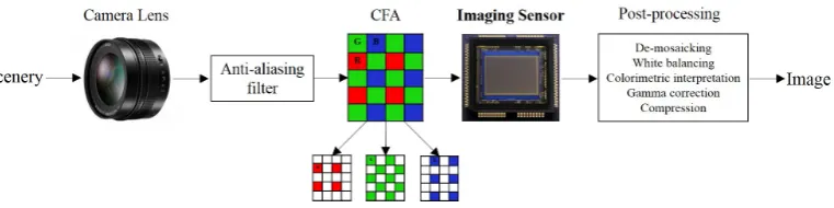
Image acquisition is actually a process of converting the incident light into a digital

(31)

[image:31.595.134.515.109.204.2]

Figure 2.1: A simplified depiction of an imaging pipeline within a digital camera.

with an ordinary digital camera is illustrated by the diagram of Fig. 2.1 [34]. The

light from the scene entering a camera is first filtered by the lens and an anti-aliasing

filter [35] before reaching the imaging sensor. The most important and expensive

part of a digital camera is the imaging sensor. Since the elements of imaging sensor

are monochromatic, each sensor element can only capture one colour value [36], such

as red (R), green (G), or blue (B). As a result, the imaging sensor can not separate

colour information. Therefore, a colour filter array is required to be built above the

imaging sensor so as to help with separating the colour information. After colour

filtering, the light is captured by the elements of imaging sensor and converted into

individual pixels that comprise the image. Later, a demosaicing operation, which is

tailored for the type of colour filter array by the camera manufacturer, takes place

to calculate the missing colour values for each pixel so as to generate a full-colour

image (with intensities of all three primary colours at each pixel). This is followed

by a sequence of post-processing operations, such as white balancing operation,

colourimetric interpretation, and gamma correction [37]. At the end, the generated

image is compressed and saved in the camera’s memory.

Among various stages of image acquisition process described above, the

(32)

pattern noise is produced. In this stage, each element of the imaging sensor would

capture the incident light and convert it into an individual digital pixel. Due to the

non-homogeneity of silicon wafer, normally different sensor elements have different

sensitivity to light. As a result, even if the imaging sensor takes an image of an

absolutely evenly lit scene, the resulting image would still exhibit slight variations

in the intensity between the individual pixels [38]. Such variations between

indi-vidual pixels form a noise pattern, which is called the sensor pattern noise. As

reported in [6], if a camera takes multiple images of exactly the same scenery, the

SPN patterns left in these images would stay approximately similar. It indicates

that every image or video taken by the same sensor would exhibit the same SPN

pattern. In addition, because of the imperfections during the sensor manufacturing

process, even two imaging sensors made from the same silicon wafer would exhibit

uncorrelated SPN patterns. As a result, the SPN produced by each sensor is unique.

Due to these proprieties, the SPN pattern can be viewed as a uniquefingerprint of

a digital camera. Its uniqueness allows SPN to distinguish not only different camera

models of the same brand, but also individual cameras of the same model.

Sensor pattern noise consists of two main components: fixed pattern noise

(FPN) and photo-response non-uniformity (PRNU) noise [39]. FPN refers to

pixel-to-pixel differences when the sensor array is not exposed to light. It is primarily

caused by dark currents. FPN is an additive noise, thus some middle-end and

high-end cameras can automatically suppress this noise by subtracting a dark frame from

every image they take [24]. On the other hand, PRNU noise is the discriminative

part of SPN. The PRNU noise is a multiplicative noise [6], and its amplitude

(33)

the observed image is, the stronger the PRNU noise would be. However, the

PR-NU noise cannot be present in completely saturated images or image areas because

the pixels were filled to their full capacity, thus a saturated image would carry no

information about the PRNU noise. For the same reason, the PRNU noise is very

weak in dark areas, leaving the FPN as the dominant component of the SPN.

2.2 SPN Extraction

As mentioned in Chapter 1.3, in order to verify whether a query image was taken

by a specific camera using SPN, three main steps are required: SPN extraction,

reference SPN estimation and SPN matching. In this section, we first introduce the

SPN extraction step, the purpose of which is to extract the SPN from the query

image. In [6], Lukaset al. modelled the output of a camera in a simplified form:

I= (1 +K)I(0)+Θ=I(0)+I(0)K+Θ, (2.1)

where I(0) is the sensor output in the absence of noise. The multiplicative factor

Krefers to the PRNU factor (K<1). I(0)Kthereby represents the discriminative

part of SPN, which is the signal of interest. Θ is the composite of independent

random noise components, which includes the dark current, shot noise, read-out

noise, and quantization noise. In the rest of this thesis, matrices are shown in

capital bold; vectors are presented in bold lower-case; operations and variables are

in element-wise.

In order to extract the signal of interestI(0)Kfrom the observed dataI, the

host signal I(0) should be removed. However, the noiseless image I(0) is generally

(34)

output. Nevertheless, it is possible to obtain an approximation to the noiseless

image I(0) by using a denoising algorithm, ˆI(0) = F(I), where ˆI(0) is a denoised

version of the imageI,F indicates the denoising algorithm. Therefore, SPN can be

estimated as the noise residual between the observationI and its denoised version

ˆ_I(0)_{. For example, by subtracting the denoised version}_ˆ_I(0) _{from the observation} _I,

we can extract an approximation of SPN as

X=I−F(I) =I−ˆI(0)

=I(0)−ˆI(0)+I(0)K+Θ=IK+Ξ, (2.2)

where X is the noise residual where the true SPN signal is present. The noise Ξ

is a sum of Θ and the additional noise terms introduced by the denoising filter.

From this equation, we can deduce that the closer the denoised versionˆI(0) is to the

noiseless imageI(0), the purer SPN signal would be extracted in the noise residual

X. Therefore, the performance of an SPN extractor is primarily determined by the

choice of the denoising algorithm F.

2.2.1 Denoising Algorithm

Since the denoising algorithm plays an important role at determining the quality

of the extracted SPN, the potential choices for the denoising algorithm is worth

further discussing. According to the works proposed by the previous researchers,

there are three most popular techniques: Mihcak filter [40], SPN predictor based on

context adaptive interpolation (PCAI) [11, 12] and block-matching and 3D filtering

(35)

Mihcak Denoising Filter

In [6], Lukas et al. pointed out that SPN is a high-frequency signal in an image,

thus they proposed to transform the noisy image I into wavelet transform domain

and apply a wavelet-based denoising filter (Mihcak denoising filter [40]) to extract

the SPN components from the high frequency wavelet coefficients of I. Since this

method [6] was the firstly proposed in literature for SPN extraction, we refer it as

“Basic” method in this thesis.

As mentioned in [6], the authors had tested with several denoising filters and

eventually decided to use the Mihcak denoising filter as it provided the best

re-sults. The underlying hypothesis of this method is that the high-frequency wavelet

coefficients of a noisy image can be modelled as an additive mixture of a locally

stationary i.i.d. signal with zero mean (noise-free image) and a stationary white

Gaussian noise (WGN) signal with variance σ₀2 (i.e. the SPN). Based on this

hy-pothesis, the Mihcak denoising filter is built in three steps. In the first step, the

input noisy image is processed by the wavelet decomposition. In the second step, the

local image variance is estimated. Finally, the local Wiener filter is used to obtain

an estimate of the denoised image in the wavelet domain. The individual steps are

described as follows:

Step 1. Wavelet decomposition. Calculate the fourth-level wavelet decomposition of

the noisy image with the 8-tap Daubechies QMF. We describe the procedure

for one fixed level (it is executed for the high-frequency bands for all four

levels). Denote the vertical, horizontal, and diagonal subbands as h(i, j),

(36)

decomposition level.

Step 2. Local variance estimation. In each subband, estimate the local variance

of the noise-free image for each wavelet coefficient using the Maximum

A-Posteriori Probability (MAP) estimation [41] for four sizes of a squarem×m

neighbourhood Nm (where m∈ {3,5,7,9}), such as

ˆ

σ_m2(i, j) =max 

0,

1

m2 X

(i,j)∈Nm

h2(i, j)−σ₀2 

,(i, j)∈J. (2.3)

The local variance of the noise-free image ˆσ2(i, j) is obtained by taking the

minimum of the four variances

ˆ

σ2(i, j) =min(σ₃2(i, j), σ₅2(i, j), σ2₇(i, j), σ₉2(i, j)),(i, j)∈J. (2.4)

Step 3. Wiener filtering. In each subband, denoise the wavelet coefficients by using

a pixel-wise adaptive Wiener filter based on the estimated local variance

from the neighbourhood of each pixel, such as

hden(i, j) =h(i, j)

ˆ

σ2(i, j) ˆ

σ2₍_{i, j}_{) +}_σ2 0

, (2.5)

where ˆσ2(i, j) is the estimated variance of the noise-free image and σ₀2 is

the variance of the WGN signal. Similarly, vden(i, j), and dden(i, j) can be

obtained in the same way, where (i, j)∈J. By repeating Steps 1-3 for each

level and each colour channel, a denoised image can be finally obtained in

the spatial domain by applying the inverse wavelet transform to the denoised

(37)

Notice that the parameterσ0is still unknown. As reported in [6], σ0 is normally set

toσ0 ∈ {1, ...,6} so as to better extract the SPN signal, and within this range, the

choice of σ0 has a relatively low impact on the final identification results. But for

the images with large noise components, such as images with strong scene details

and images which are highly compressed, settingσ0 to a relatively large value would

make sure that the filter extracts a substantial part of the SPN. For this reason, we

have chosenσ0 = 4 in all the following experiments of this thesis. Based on the Eq.

(2.2), this Basic method can be simply formulated as follows

X=DW T−1{DW T(I)−F[DW T(I)]}, (2.6)

whereDW T is the discrete wavelet transform, and DW T−1 is the inverse wavelet

transform. F is the Mihcak denosing filter, which is constructed in the wavelet

domain using the Wavelab package [42].

PCAI Predictor

In [12], Wuet al. proposed an edge adaptive predictor based on the context adaptive

interpolation (PCAI) to extract SPN. Since the scene texture is the most serious

source that contaminates the true SPN signal, this PCAI method was designed

mainly to suppress the impact of scene texture. The context adaptive interpolation

(CAI) method [43] is an interpolation method which can predict the texture within

an image by using the local neighbouring information. However, subtle signal, such

as SPN, is not very likely to be accurately predicted in the output by this method.

(38)

the impact of image edges while preserving the SPN components at the same time.

• The CAI interpolation method. Assume that p is the central pixel and

t={n, s, e, w}T _{is the vector of neighbouring pixels. The CAl interpolation method}

would predict an approximation ˆpfor the pixel valuepaccording to its neighbouring

informationt. More specifically, the CAl method firstly scans the whole image and

classifies each pixel (according to its local region) into four categories: smooth,

horizontally-edged, vertically-edged and other. In the smooth region, a mean filter

is used to estimate the central pixel; in edged regions, the interpolation is done along

the edge; otherwise a median filter is applied. The predicted pixel value ˆp can be

formulated as follows [43]

ˆ p=                         

mean(t), (max(t)−min(t)≤20)

(n+s)/2, (|e−w| − |n−s|>20)

(e+w)/2, (|n−s| − |e−w|)>20)

median(t), (otherwise).

(2.7)

In Eq. (2.7), the central pixel, which is predicted according to different types of edge

regions, is classified by the four-neighbouring pixel values with a threshold value.

According to [12], this threshold is set to be 20 via the extensive experiments. In [11],

the CAI method is extended by using of the eight-neighbouring pixels (including

four diagonally-edged pixels), which is called as “CAI8”. By doing so, the authors

claimed that the predicted result ˆpwould have less prediction error [11].

• The PCAI predictor. In [11], an edge adaptive SPN predictor is proposed

(39)

This PCAI8 predictor is built in two steps as follows.

Step 1. Firstly, the CAI8 method is applied as the desnoising filterF in Eq. (2.2).

Then, the differenceD between the predicted result and original image can

be calculated in the spatial domain as follows

D=I−CAI(I), (2.8)

where CAI(I) is a pixel-wise prediction of the original image I. The CAI

method can only predict the scene texture ofIbut not the SPN components.

Therefore, the scene texture would be suppressed in the differenceD while

the SPN components would be well preserved.

Step 2. In order to further suppress the impact of the scene texture and extract a

more accurate SPN, a pixel-wise adaptive Wiener filter is then preformed

as follows [11]

X(i, j) =D(i, j) σ

2 0 σ2₍_{i, j}_{) +}_σ2

0

, (2.9)

whereXis the eventual output of the PCAI8 predictor and the noise

resid-ual that contains the SPN components. σ2 indicates the estimated local

variance of the noise residualD and σ₀2 is the variance of the WGN signal,

i.e. the SPN. The local variance is estimated by using the MAP estimation,

which is similar to Eq. (2.4) and (2.5). The parameter σ0 is also set to be

4 in order to extract a consistent level of the SPN.

Since the CAI method can predict texture accurately according to different local

(40)

from the images with strong scene details [43]. However, due to the pixel-wise

interpolation, this method is more computationally complex.

BM3D Denoising Filter

In [8], Chierchiaet al. proposed to replace the Mihcak filter with a more recent

tech-nique, namely the block-matching and 3D filtering (BM3D) [44], in order to extract

SPN. BM3D works through grouping 2D image patches with similar structures into

3D arrays and collectively filtering the grouped image blocks. The sparseness of the

representation due to the similarity between the grouped blocks makes it capable

of better separating the noiseless image and noises. This filter is constructed using

two steps as follows:

Step 1. Basic estimate. The input noisy image is processed by successively

extract-ing the reference blocks from the image (in a slidextract-ing-window manner,e.g.,

8×8).

a) Block-wise estimates. For each reference block in the noisy image, find

the blocks that are similar to the currently processed one and then stack

them together in a 3D array (group). Then, apply a 3D transform to the

formed group, attenuate the noise by a hard-thresholding of the transform

coefficients, invert the 3D transform to produce estimates of all grouped

blocks, and return the estimates of the blocks to their original positions.

b)Aggregation. Compute the basic estimate of the true-image by a weighted

averaging of all the obtained block-wise estimates that are overlapping.

(41)

collaborative Wiener ltering.

a)Block-wise estimates. For each block, use block-matching within the basic

estimate to find the locations of the blocks similar to the currently processed

one. Using these locations to form two groups (3D arrays), one from the

noisy image and one from the basic estimate. Then, apply a 3D transform

on both groups. Perform Wiener filtering withσ0 = 4 on the noisy one using

the variance of the basic estimate as the true variance. Produce estimates

of all grouped blocks by applying the inverse 3D transform on the filtered

coefficients and return the estimates of the blocks to their original positions.

b) Aggregation. Compute a final estimate of the true image by aggregating

all of the obtained local estimates using a weighted average.

Generally speaking, among the three aforementioned SPN extraction methods, the

BM3D method can slightly outperform the Basic and PCAI8 method on SPN

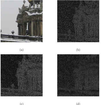
ex-traction. For the example in Fig. 2.2, (a) shows an image with strong scene details.

(b), (c) and (d) are the noise residuals extracted from the image of (a) by using

the Basic, PCAI8 and BM3D method, respectively. By comparing (b), (c) and (d),

we can see that the BM3D method can better suppress the impact of scene details

than the Basic and PCAI8 counterparts. It is because both of the Mihcak filter and

PCAI8 predictor estimate the variance of noise-free image by using only the local

neighbourhood information, while the estimate of BM3D filter is obtained by

collab-oratively aggregating the estimates from multiple non-local blocks. The denoising

output F(I) from BM3D filter is, therefore, closer to the true noise-free image I0_.

(42)

(a) (b)

[image:42.595.146.499.116.483.2]

(c) (d)

Figure 2.2: (a) An image with strong scene details. (b) The noise residual extracted from the image (a) using the Basic method. (c) The noise residual extracted from the image (a) using the PCAI8 method. (d) The noise residual extracted from the image (a) using the BM3D method. Note the intensity of (b), (c) and (d) has been downscaled 3 times for visualization purpose.

Moreover, there are some SPN extraction methods proposed in allusion to

eliminating specific contaminations. For example, Liet al.[10] introduced a

colour-decoupled PRNU (CD-PRNU) extraction method to prevent the interpolation noise

from propagating into the physical components. They extracted the PRNU noise

(43)

CD-PRNU. In [46], Al-Aniet al. developed another image denoising algorithm for

SPN estimation. The authors claimed that involving a large number of pixels at the

denoising operation to approximate a single pixel would result in a considerable level

of unwanted correlation between neighbouring pixels in the extracted noise residual.

As a result, the obtained noise residual cannot well manifest the characteristic of the

true SPN components. In order to suppress the correlation between neighbouring

pixels in the extracted noise residual, they proposed to produce a noise estimate of

SPN at a pixel via subtracting this pixel by one adjacent pixel which has a close

value.

2.2.2 SPN Enhancement

As shown in Eq. (2.2), the extracted noise residual contains not only the true SPN

components but also some unwanted interferences, such as random noise

compo-nents, scene details, CFA artifacts, etc. Thus it leaves room for further

enhance-ment.

In [9], Li pointed out that the contaminations from scene details is the most

serious one among these interferences, the magnitude of which is far greater than

that of true SPN signal. Since the scene details also account for the high-frequency

components of I, it would mix with the true SPN signal and be extracted into

the noise residual at the same time. As shown in Fig. 2.2, the scene textures

appearing in Fig. 2.2 (a) propagate through the three SPN extraction methods into

the noise residual and contaminate the true SPN signal. Although BM3D filter is

reported that can better suppress the impact of scene details, there are still some

(44)

[image:44.595.147.495.96.298.2]

(a) (b)

Figure 2.3: (a) The noise residual extracted by using the Basic method. (b) The enhanced version of (a) by using the Model 5 in [9]. Note the intensity of (a) and (b) has been down scaled 3 times for visualization purpose.

residuals would lead to two noise residuals being correlated even though they are

derived from different cameras. As a result, it would increase the false identification

rate. To overcome this limitation, Li [9] proposed an SPN enhancer to attenuate the

impact of scene details so as to enhance the true SPN signal in noise residual. The

hypothesis underlying his SPN enhancer is that the stronger a signal component inX

is, the less trustworthy the component should be, and thus it should be attenuated.

According to this hypothesis, the author provided 5 spatial-domain based enhancing

models aiming at assigning less significant weighting factors to strong components

ofX so as to attenuate the interference of scene details. Here is an example shown

in Fig. 2.3, where Fig. 2.3 (a) is the noise residual extracted by using the Basic

method, and Fig. 2.3 (b) is the enhanced version of (a) by using the Model 5 in [9].

We can clearlys see that the trace of scene details left in Fig. 2.3 (a) has been

significantly suppressed in Fig. 2.3 (b). It suggests that this enhancement scheme

(45)

enhance the purity of the SPN components in the noisy noise residual.

In [47], Lawgaly et al. proposed an enhancement method based on the

Un-sharp Masking technique [48], which aims to amplify the high frequency content of

the SPN in images. This method can strengthen the SPN present in images and

consequently enhance the SPN components in the estimated noise residuals. It can

be applied as a pre-processing method performed before the SPN extraction.

Moreover, there are some methods proposed to suppress the contamination

caused by JPEG compression. In JEPG compression, non-overlapping 8×8 pixels

blocks are coded with the discrete cosine transform (DCT) independently [49]. As a

result, aggressive JPEG compression would cause blocky artifacts in the extracted

noise residual. In [50, 51], Alles et al. proposed a method to suppress the JPEG

block artifacts by averaging neighbouring 8×8 pixels block into one macro

ele-ment on both the query noise residual and reference SPN. By doing so, the sizes

of the query noise residual and reference SPN are decreased. While this method

can attenuate the impact of JPEG blocky artifacts, it also suppresses the true SPN

components. In [52], Chen et al. proposed a more robust method to remove the

JPEG blocky artifacts by transforming the extracted noise residual into the discrete

Fourier transform (DFT) domain and suppressing the Fourier coefficients with

ex-tremely larger magnitude. By doing so, they claimed that not only JPEG blocky

artifacts but also other artifacts which manifest themselves as peaks in the Fourier

domain (e.g., artifacts due to colour filter array interpolation and other hardware

or software operations) can be suppressed.

Certainly, the methods for SPN extraction and SPN enhancement can be

(46)

algorithm to extract the raw noise residual, and then enhance it with the help of

Li’s models [9].

2.3 Reference SPN Estimation

The reference SPN estimation step aims at estimating a reference SPN pattern for

the camera in question. In [6], Lukas first proposed to estimate the reference SPN

Rfor a camera by averagingN noise residuals extracted from the reference images

taken by that camera, such as

R=XN

i=1Xi/N.

(2.10)

Generally speaking, random noises presented in different images are normally quite

different, while the true SPN components will be the same as long as these images

are taken by the same camera. Therefore, the random noise components (e.g. shot

noise, read-out noise and quantization noise) can be averaged out in R while the

true SPN components are accumulated. It is obvious that the larger the number

of imagesN is, the more random noise components we can suppress. As suggested

in [6], it is optimal to set N > 50. It is worth noting that if the camera to be

identified is available, it is better to use the low-variation images such as blue sky

and flat field images for reference SPN estimation, so that we can actively avoid the

contaminations caused by scene details. By doing so, we actually incorporate our

prior knowledge of SPN to refine the estimated result.

In [7], Chen et al. proposed a maximum likelihood method to estimate the

(47)

is a multiplicative noise, thus the goal of this method is to estimate the reference

PRNU factor Kfor a camera. They assume that the pixels of the noise term Ξ is

zero-mean Gaussian noise with varianceσ2and independent from the signalIK. Let

{Ii}N_i₌₁ be the reference images from camera C. For each image Ii,i = 1,2, ..., N,

the Eq. (2.2) can be re-written as:

Xi

Ii

=Ki+

Ξi

Ii

, where Xi=Ii−F(Ii). (2.11)

Finally, the reference PRNU factor for cameraCcan be estimated by the Maximum

Likelihood estimation:

ˆ

K=

PN i=1XiIi PN

i=1I2i

. (2.12)

Now given a query image Iq, this method [7] would regard the term IqKˆ as the

reference SPN left in imageIq by cameraC.

In [53], Huet al. pointed out that the components of the reference SPN with

larger values are more robust. Therefore, instead of using the full-size reference SPN,

authors only select a small number of the largest components from it as the reference.

Moreover, they also record the location information of these largest components so

that they can select the corresponding components from the query SPN to perform a

matching. This method works very well when the reference SPN is clean. However,

its performance would degrade when the reference SPN is contaminated by scene

details, because the large components in such a contaminated SPN is more likely to

be associated with scene details rather than true SPN components.

To further refine the estimated reference SPN, Chenet al. [7] proposed two

(48)

dis-crete Fourier transform (DFT) domain, to remove the artifacts caused by camera

processing operations from the reference SPN. The ZM procedure is to remove the

artifacts introduced by CFA interpolation, row-wise and column-wise operations of

sensors or processing circuits. The objective of the WF procedure is to suppress the

visually identifiable patterns in the ZM processed signal. These two pre-processing

operations can be summarized as follows

RW F =DF T−1(DF T(RZM)−F(DF T(RZM))), (2.13)

in which DF T is the discrete Fourier transform, DF T−1 is the inverse discrete Fourier transform. F is the Wiener filter with the variance obtained as the sample

variance of the magnitude of theDF T(RZM).

In [54], another reference SPN pre-processing approach, namely the

Spec-trum Equalization Algorithm (SEA), is recently proposed to suppress the periodic

artifacts, such as CFA interpolation artifacts, JPEG blocky artifacts and diagonal

artifacts, from the estimated reference SPN. The authors claimed that the peaks

appearing in the DFT spectrum are probably originated from the periodic artifacts

and unlikely to be associated with the true SPN. Therefore, by detecting and

sup-pressing the peaks in the DFT spectrum, the reference SPN of better quality can

(49)

2.4 SPN Matching

Once both query SPN and reference SPN are obtained, the SPN matching step is

finally performed to measure the similarity between the query SPN and the reference

SPN so as to decide whether the query image was taken by the camera in question.

This problem can be treated as a binary-hypothesis test with the two hypotheses [55],

which are defined as

H0 :X6=R(the query image is not taken by the suspect camera)

H1 :X=R(the query image is taken by the suspect camera)

Then a correlation-based detector is used to make the decision betweenH0 and H1

by comparing the correlationρ(X,R) to a pre-calculated thresholdτ. The detector

decidesH1 when ρ>τ andH0 whenρ < τ.

2.4.1 Similarity Measurement

For this type of problem, the normalized cross-correlation (NCC) is usually used as

the similarity measurement (detection statistics) to measure the similarity between

the query noise residual and the reference SPN, which is defined as:

ρ(X,R) =

PN i=1

PN

j=1 X(i, j)−X

R(i, j)−R

X−X

·

R−R

, (2.14)

whereX andRare the mean value ofXandR,N×N is the size ofXand R, and

k·kis the L2 norm. Later, Goljan et al. [56] pointed out that the normalized

cross-correlation is sensitive to the influence of periodic noise contaminations, therefore

(50)

ratio [57], to suppress periodic noise contamination, such as

P CE(X,R) = C

2

RX(0,0) 1

N2_−|_A_|

P

(i,j)∈/ACRX2 (i, j)

, (2.15)

whereC_RX2 is circular cross-correlation between the two fingerprintsXandR,Ais a

small area around (0,0), and|A|is the size ofA. In the real-world applications, when

the final decision will be served as a vital piece of evidence in a crime investigation,

a low false positive rate (FPR) is usually required so as to ensure a low probability

of wrong accusation. Therefore, Kang et al. [13] proposed a more sophisticated

detection statistic, i.e., the correlation over circular correlation norm (CCN), to

further reduce the FPR of a source camera identification system, such as

CCN(X,R) = _q CRX(0,0) 1

N2_−|_A_|

P

(i,j)∈/ACRX2 (i, j)

. (2.16)

2.4.2 Detection Threshold

The accuracy of a SCV or SCI system is defined by true positive rate (TPR) and

false positive rate (FPR). True positive rate is the probability of decidingH1 while

hypothesisH1 is true, and false positive rate is the probability of deciding H1 while

H0 is true. Investigators usually require an SCV or SCI system to have a sufficiently

low FPR so as to ensure a low probability of wrong accusation in some real-world

applications, such as child pornography cases. Therefore, the detection thresholdτ

(51)

According to Eq. (2.2), we simplify and rewrite it into a vectorized form as:

x=xˆ+ξ, (2.17)

wherexindicates the noise residual,ˆxpresents the true SPN signal andξ is WGN.

Following the assumptions of [58], we assume that the noise residuals to be matched

are normally distributed random sequences with zero mean and unit variance such

thatx={xi}={xˆi+ξi},i= 1, ..., m, whereξi ∼ N(0, σ2), ˆxi∼ N(0,1−σ2) andm

is the length of the vectorized noise residual. We also assume that SPNs of two

dif-ferent cameras are statistically independent. According to the central limit theorem

(CLT) [59], the NCC values for independent vectors follow the Gaussian

distribu-tion. Therefore, from the independence of SPNs assumption, the distribution of the

NCC values for non-matching SPNs (under hypothesis H0) can be approximately

estimated as a normal distribution with zero mean and variance equal to 1/m, i.e.,

ρH0 _{∼ N}₍₀_,₁_/m_{). Given a detection threshold, the false positive rate} _P

f p for SPN

can be obtained via Neyman-Pearson hypothesis approach [60] as follows

Pf p=Q(τ √

m), (2.18)

where Q is the complementary cumulative density function of a normal random

variableN(0,1). Given a requiredPf p, the detection threshold can be obtained via

an inverse operation as

τ = Q −1₍_P

f p) √

m , (2.19)

Learning based forensic techniques for source camera identification

warwick.ac.uk/lib-publications

A Thesis Submitted for the Degree of PhD at the University of Warwick

Permanent WRAP URL:

http://wrap.warwick.ac.uk/86799

Copyright and reuse:

This thesis is made available online and is protected by original copyright.

Please scroll down to view the document itself.

Please refer to the repository record for this item for information to help you to cite it.

Our policy information is available from the repository home page.

Learning based Forensic Techniques for

Source Camera Identification

Ruizhe Li

Computer Science

Contents

Acknowledgments

Declarations

Abstract

Abbreviations

List of Tables

List of Figures

Chapter 1

Introduction

1.1

Background

1.2

Source Camera Identification

1.3

SPN-based Source Camera Verification and

Identi-fication

1.4

Challenges

1.5

Objectives of Thesis

1.6

Thesis Outline

1.7

List of Publications

Chapter 2

Literature Review

2.1

Image Acquisition Process

2.2

SPN Extraction

2.3

Reference SPN Estimation

2.4

SPN Matching