Some problems in irregular ordinary differential equations

University of Warwick institutional repository: http://go.warwick.ac.uk/wrap

A Thesis Submitted for the Degree of PhD at the University of Warwick

http://go.warwick.ac.uk/wrap/55877

This thesis is made available online and is protected by original copyright.

Please scroll down to view the document itself.

Some problems in irregular ordinary differential

equations

by

Nicholas Sharples

Thesis

Submitted to the University of Warwick for the degree of

Doctor of Philosophy

Mathematics Institute

March 2012

Contents

Acknowledgments

Declarations

Abstract

Chapter 1 Introduction

Chapter 2 Ordinary Differential Equations

2.1 Classical solutions . . . .

...

2.1.1 Dependence on initial conditions, the transport equation and

iv v vi 1 7 7

the continuity equations . . . 9 2.1.2 Existence and uniqueness of flows: Lipschitz vector fields

2.1.3 Compressibility... 2.1.4 Fractal geometry . . . . 2.1.5 A flow into a Cantor set Generalised solutions . . . . 2.2

2.3 2.4

Existence of regular Lagrangian flows .

From regular Lagrangian flows to absolutely continuous flows 2.4.1 A related result in the theory of Sobolev maps

Chapter 3· Uniqueness

3.1 Trajectory non-uniqueness. 3.1.1 A scalar example .. 3.1.2 A planar example

3.2 A general non-uniqueness result .

3.2.1 Vector field redefinition and avoidance Chapter 4 A voidance

4.2 Avoidance criteria . . . .

...

Chapter 5 Dimension prints

5.1 r-codimension print . . . . 5.1.1 Properties of the r-codimension print .. . 5.1.2 Relationship with box-counting dimension . 5.1.3 Product sets

5.1.4 Examples ..

Chapter 6 Box-counting dimension 6.1 Box-counting dimension . . .

6.1.1 Equivalent definitions .. 6.1.2 Product sets . . . . 6.2 Compatible generalised Cantor sets .

6.2.1 Geometry of generalised Cantor sets 6.2.2 Box-counting dimension . . . .

56 64 66 68 69 74 80 83 83 85 87 91 93 97

Chapter 7 Function spaces and measurability 103

7.1 Definitions of the £P spaces . . . . 105 7.1.1 Measurability and strong measurability 105 7.1.2 Spaces of maps £P (A; X) . . . . 106 7.1.3 Spaces of equivalence classes LP (A; X) . 108 7.2 £P (I; £P (D)) and £P (I x D) as equivalence classes of real valued maps. 108 7.2.1 A characterisation of £P (I; LP (D)) for 1

:S

p

:S

00. . 109 7.2.2 Equivalence classes of £P (I x D) and £P (I; £P (D)). 115 7.3 Inclusions between LP (I x D) and £P (I; £P (D)) ..

7.4 Inclusions between VXJ _{(I x D) and L}OO _{(I; L}oo _{(D)) .} Chapter 8 Addendum: Continuity of Sobolev Maps

8.1 An application to non autonomous Sobolev spaces. Chapter 9 Conclusion

Appendix A Measure theory

117 123 128 131 135 139

Appendix B Precise representatives and absolutely continuous maps141 B.1 Lebesgue points and precise representatives . . . 141 B.2 Sobolev maps. . . 142 B.3 Mollifiers and the precise representative of Sobolev maps. 142

B.4 Absolutely continuous maps List of Symbols

...

144

Acknowledgments

I wish to thank the Engineering and Physical Sciences Research Council for their generous financial support. Further, it is a pleasure to thank James Robinson for his guidance, insight and friendship throughout my studies at the University of Warwick. Finally, I owe my deepest gratitude to my family and friends for their support over the years leading to the writing of this thesis, and in particular to the wonderful Isabelle for her support and love, and for making it all worthwhile.

Declarations

I declare that the work in this thesis was carried out in accordance with the Regu-lations of the University of Warwick. The work is original except where indicated by special reference in the text and no part of the thesis has been submitted for any other degree.

Abstract

We study the non-autonomous ordinary differential equation

x

=

f

(t, x) in the situation when the vector field

f

is of limited regularity, typically belonging to a space LP (O,T; Lq (JRn)). Such equations arise naturally when switching from an Eulerian to a Lagrangian viewpoint for the solutions of partial differential equations. We discuss some measurability issues in the foundations of the theory of regular Lagrangian flow solutions. Further, we examine the sensitivity of the choice of representative vector field

f

on solutions of the ordinary differential equation and, in particular, we demonstrate that every vector field can be altered on a set of measure zero to introduce non-uniqueness of solutions.

We develop some geometric tools to quantify the behaviour of solutions, notably a non-autonomous version of subset avoidance and the r-codimension print that encodes the dimension of a subset S

c

JRn x

[0,

T] while distinguishing between the spatial and temporal detail of S. We relate this notion of dimension to the more familiar box-counting dimensions, for which we prove some new inequalities.

Finally, motivated by the issues with measurability that can arise with ir-regular vector fields we prove some fundamental results in the theory of Bochner integration in order to be able to manipulate the representatives of the equivalence classes in LP (O,T; Lq (JRn)).

Chapter

1

Introduction

This thesis is concerned with the study of the non-autonomous ordinary differential equation

d~~t)

=

f

(~(t),

t) (1.1 ) when the vector field f: JRn x [0, T] - t JRn is not necessarily continuous but is measurable and sufficiently integrable to belong to the space V (0, T; Lq (JRn)) for some 1 ~ p, q ~ 00. Such problems arise naturally when switching from an Eulerian

to a Lagrangian viewpoint for the solutions of partial differential equations which can have only very limited regularity, such as the Navier-Stokes equations.

In Chapter 2 we discuss the foundations of the theory of irregular ordinary dif-ferential equations. We recall some elements of the classical. theory, where typically the vector field

f

is continuous and the objects of study are classical flow solutions of (1.1). In this familiar setting we introduce the concepts of solution concatenation and the avoidance of sets by classical flow solutions, which we develop for irregular ordinary differential equations in Chapters 3 and 4. In Section 2.2 we follow the seminal paper of DiPerna and Lions [1989] and the refinements in Ambrosio [2004] and De Lellis [2008] to motivate and discuss the appropriate notion of solution of (1.1) when the vector field is merely integrable. In particular we note that a classical flow solution is too strong to be of use for two reasons: firstly, a classical solution ~

requires the vector field

f

to be continuous on the trajectory

f

(~(t),

t),

which is a strong restriction for vector fields that are only assumed to be integrable. Secondly, we recall that the elements of the space V (0, T; Lq (JRn)) are equivalence classes of maps that are equal almost everywhere. Consequently, in order to be able to use the tools of functional analysis to find solutions of (1.1) we require that solutions are invariant under a choice of representative of the equivalence class of

f.

An appropriate notion of solution of (1.1) in the irregular setting, identified in DiPerna and Lions [1989] and developed in Lions [1998], Ambrosio [2004]' Hauray et al. [2007], De Lellis [2008] and others, is that of a regular Lagrangian flow solution, which we detail in Definition 2.32. Roughly, a regular Lagrangian flow solution is an integrable map X: [0, T] x lRn x [0, T] -+ lRn satisfying

r

T

d¢

r

T

Jo X(t,x,s) dt (t)dt+ Jo !(X(t,x,s),t)¢(t)dt=O

for all test maps ¢ E

ego

((O,T)), for almost every (x,s) E lRn x [O,T] with the additional Lusin property that for every Borel set A

c

lRn of zero measure the set {x E lRnlX

(t,

x, s) E A} has zero measure for almost .every

t

E [0, T] and almost every s E [0,

T].

Essentially, this property guarantees that spatial sets of positive measure are not transported under the action of the flow into sets of zero measure.

In the example of Section 2.1.5 we describe a classical flow solution that does not have the Lusin property, illustrating that regular Lagrangian flows are not strictly a generalisation of classical flows.

In DiPerna and Lions [1989] the authors demonstrate that a regular La-grangian flow solution X necessarily has some Sobolev regularity with respect to time. Further, as one dimensional maps with Sobolev regularity have absolutely con-tinuous representatives the authors conclude that there is a representative of X that is absolutely continuous in time, simplifying much of the theory. In Section 2.4 we de-scribe this argument and examine a potential obstruction: we claim that if X is a reg-ular Lagrangian flow solution of (1.1) then there is a map X: [0,

T]

xlRn x [0,

T]

-+ lRn such that

• for almost every (x, s) E lRn _{x [0,}

_T]

_{the map t t-+}

_X

_{(t, x, s) is absolutely}

continuous, and

• X(t,x,s) = X(t,x,s) for almost every t E [O,T] for almost every (x,s) E lRn x

[0,

T]

however, we argue that it does not follow that the map X is equal to X almost everywhere on [0,

T]

x lRn x [0,

T].

In particular, the map

X

may not be measur-able, in which case we are unable to consider the measure of the inverse images X-I

(t,.,

s) A which are significant to the theory of regular Lagrangian flows. For-tunately, in Chapter 8 which was completetd after the submission of this thesis, we are able to demonstrate that the map

X

is measurable. We end the chapter by discussing a similar problem in a classical result from the theory of Sobolev maps, and how adapting the proof of this result may remove the obstruction to the theory

of regular Lagrangian flows. We discuss the sensitivity of choosing representatives of equivalence classes in a more general setting and at greater length in Chapter 7. In the remainder we use the result of Chapter 8 that guarantees there is a measurable absolutely continuous representative of each regular Lagrangian flow and we restrict ourselves to this representative. With the additional regularity of this representative a map X is a regular Lagrangian flow solution of (1.1) if it sastisfies the Lusin condition and for almost every (x, s) E jRn x [0,

T]

X(t,x,s)=x+

l

tf(X(T,x,s),T)dT VtE[O,T],

which is the definition used in Lions [1998], Hauray et al. [2007], Crippa and De Lellis [2008], and others. With this formulation we can regard the map X as an aggregate of absolutely continuous solutions, with one solution for almost all initial data.

In Chapter 3 we discuss the uniqueness of absolutely continuous solutions of (1.1). We revisit the technique of solution concatenation and demonstrate in Theorem 3.1 that the concatenation of any absolutely continuous solutions is itself a solution. As a consequence, we see that examples of vector fields with non-unique solutions are easy to construct: we give two examples of vector fields with arbitrary Sobolev regularity (that is in Wk,oo (jRn; jRn) for all kEN) such that there are non-unique solutions for all initial data.

In Theorem 3.4, which is the main result of Chapter 3, we illustrate that the uniqueness of solutions is sensitive to the choice of representative vector field

f.

We prove that if there exists a regular Lagrangian flow solution of (1.1) then there is a vector field equivalent to 9 such that the ordinary differential equation ~ = 9 (~, t) has non-unique solutions on a set of initial data of positive measure. We end the chapter by demonstrating that if (1.1) has a regular Lagrangian flow solution X and unique solutions for almost all initial data, and if the set

N:= {(x, t) E jRn x

[0,

Tllf

(x, t) =1= 9 (x, t)}

is sufficiently small that the flow X 'avoids' N, then the solutions of ~ = 9 (~, t) are unique for almost all initial data. An article containing the discussion and results of Chapter 3, co-authored with James Robinson, is currently in preparation.

We discuss the avoidance of subsets at length in Chapter 4 where, in Theorem 4.8, we adapt a result of Aizenman [1978b] to the non-autonomous case to give a

sufficient condition for a regular Lagrangian flow to avoid a subset S

c

JRn x [0, T].

This condition is written in terms of both the spatial and the temporal regularity of the vector field

f

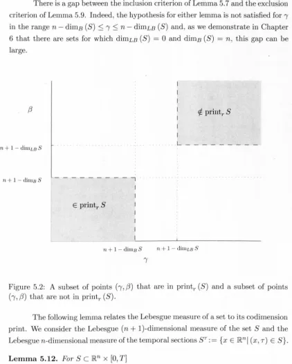
and an integral quantity dependent on the set S. In Chapter 5 we use this integral quantity to define a two-parameter 'r-codimension print', similar to the Hausdorff dimension print of Rogers [1988], which encodes the 'dimension' of the set in such a way that the temporal detail is distinguished from the spatial detail. In Theorem 5.13 we partially describe the r-codimension print of S in terms of the box-counting dimensions of the projections of S onto the coordinate axes. These results on non-autonomous avoidance and the r-codimension print are described in an article, co-authored with James Robinson, that is currently under review for publication in the Journal of Differential Equations.

Theorem 5.13 gives a partial description of the r-codimension print of a subset S, in terms of the upper and lower box-counting dimensions of its projections. In order to obtain the sharpest results for this Theorem, we need the best possible control of the upper and lower box counting dimensions of the set S and of its projections. In Chapter 6 we recall the definition of the box-counting dimension in a general metric space and in Theorem 6.8 we prove that for compact subsets F, G E JRn the upper and lower box-counting dimensions of the product set F x G satisfy

dimLB (F)

+

dimLB (G) ~ dimLB (F x G)

::; min (dimLB (F)

+

dimB (G) ,dimB (F)

+

dimLB (G)) ~ max (dimLB (F)

+

dimB (G) ,dimB (F)

+

dimLB (G)) ::; dimB (F x G)

~ dimB (F)

+

dimB (G) .

As far as we are aware the second and fourth inequalities are new. In the second half of Chapter 6, we provide a method of constructing 'compatible generalised Cantor sets'

F,

G

c

JR such that the upper and lower box-counting dimensions of F, G and the product set F x G take arbitrary values subject to the above inequalites. The results in this chapter are described in an article, co-authored with James Robinson, that has been accepted for publication in Real Analysis Exchange.

Throughout this thesis we avoid the abuse of notation in which we would write fELl (JRn) for a map f as properly the elements of this space are equivalence classes of maps. We write f E [ } (JRn) if the map f: JRn -+ JR is Lebesgue measur-able and the integral

flR

n

If

(x)

I

dx is finite. We observe that the space [,

1 _{(JRn) is}

only equipped with a semi-norm, which we denote by

11'IIO(lRn)'

In Chapter 7 we discuss Bochner integration with a view to defining and manipulating elements of the spaces £P (0, Tj U (l~n)), which feature prominently in the theory of irregular non-autonomous ordinary differential equations. An important result of Chapter 7 is that the space £1

(0,

Tj £1 (l~n)), which consists of equivalence classes of equivalence-class-valued maps, is isometrically isomorphic to a space

£.1

(0,

Tj.c1 _{(JRn)) of real} valued maps modulo the equivalence relation defined by

f

rv 9 iff

f

(t,

x) = 9

(t,

x)

for almost every x E JRn, for almost every t E

[0,

T]

is a Banach space. With this characterisation we can regard a real valued map f:

[0,

T] x JRn -+ JRn as being a representative of an equivalence class of £1

(0,

Tj £1 (JRn)).

In Section 7.2.2 we illustrate an important consequence of dealing with maps rather than equivalence classes: even though the spaces £1 ((0, T) x JRn) and

£1

(0,

Tj £1 (JRn )) are isometrically isomorphic the inclusion

is strict. Indeed, in Corollary 7.13 we demonstrate that the indicator map of a set first described in Sierpinski [1920] is in

.c

1 (0, Tj.c1 (JR

n))

but is not measurable as a map from

[0,

T] x JRn -+ lR. In particular, if

f

(x, t) = 9 (x, t) for almost every x E JRn,

for almost every t E

[0,

T] then it is not necessarily the case that

f

(x, t) = 9 (x, t) almost everywhere on JRn x

[0,

T].

In general, manipulating the 'almost everywhere' quantifier of measure theory requires caution, as we discuss in Appendix A. In this appendix we demonstrate that the only implication between statements with almost everywhere quantifiers is

p (x, y) V x, a.e. y p (x,

y)

a.e.

y,

V x,

and in fact the validity of the implication

p (x, y) a.e. x, a.e. y p (x, y) a.e. y, a.e. x,

depends upon our choice of axioms. To avoid these difficulties whenever we manip-ulate these quantifiers we will do so explicitly.

The spaces £P (0, Tj £P (JRn)) for 1 :::; p

<

00 similarly are isometrically

iso-morphic to £P ((0, T) x JRn) but this is not true of £00 (0, Tj £00 (JRn)). In Section . 7.4 we describe a simple example of a map

f,

due to Juan Arias de Reyna

(Univer-sity of Seville), that is in

.coo

([0, 1] x [0, 1]) but not in

.coo

(0, 1 j

.coo

(0, 1)). Further,

we show that no map that is equal to

f

almost everywhere on [0, 1] x [0, 1] is in

both spaces. We use this example to show that there is an isomorphism between LOO _{(0, T; L}OO _{(]Rn)) and a proper subspace of £00 ([0, T] x ]Rn).}

An article containing the discussion and results of Chapter 7 co-authored with James Robinson and Jose Real (University of Seville) is currently in preparation. Both James and I were saddened to learn of the death of Jose Real on the 27th of January 2012.

Chapter

2

Ordinary Differential Equations

Our interest is in the non-autonomous ordinary differential equation

~;

=

f(~(t),t)

(ODE)

when the vector field f: IRn x

[0,

T] -t IRn is of limited regularity, typically belonging to the space £P (0, T; Lq (IRn)) for some p, q

E [1,00].

Intimately related to (ODE) are two partial differential equations, the transport equation

au

at

+

f .

\7 xU =

°

on IRn x (0, T) (TE)

and the continuity equation

~+div(fP)=O

on IRn x (O,T). (CE)

There are two notions of solution of (ODE): trajectories, which describe a single continuous curve through the phase space IRn that satisfy (ODE) in some sense; and flow solutions, which describe an aggregate of trajectories satisfying some additional properties.

First, we recall the definitions of classical trajectories and flow solutions, where we require the vector field

f

to be continuous, before defining appropriately weakened analogues for vector fields of limited regularity.

2.1

Classical solutions

In the classical case we require a solution to the equation (ODE) to hold in the pointwise sense; for each point t E [0,

T]

we require the derivative to exist and to be

equal to the vector field evaluated at this point.

Definition 2.1. For each (x,s) E]Rn x [O,T] a map~: [o,T]-+]Rn is a solution of

(ODE) with initial data (x, s) if

• ~ is continuously differentiable on

[0,

T]

• for each t E

[0,

T] the pointwise derivative

*

=

f (~(t), t), and

• ~ (s)

=

x.

For such ~ the map t H (~(t) ,t) is called a trajectory of (ODE) with initial data

(x, s).

Note that we require the map to be defined and satisfy the equation (ODE). over the entire temporal domain. We can consider local solutions, where the map is defined on just a small neighbourhood of the initial time s but this is beyond the scope of this thesis.

There is a useful equivalent formulation in terms of integral equations: Lemma 2.2. The map ~: [0, T] -+ ]Rn is a solution of (ODE) with initial data (x, s) E ]Rn x

[0,

T] if and only if ~ is continuously differentiable and satisfies

Vt E [O,T].

A classical flow solution of (ODE) is an aggregation of a solution of (ODE) for each initial data with an additional group property:

Definition 2.3. A map X: . [0, T]t x ]R~ x [0, T]s -+ ]Rn is a classical flow solution of (ODE) if for all initial data (x, s)

• X (., x, s) is continuously differentiable on [0, T], and

• X(t,x,s)=x+istf(X(r,x,s),r)dr

V

t E

[0, TJ,

and further the map X satisfies the group property

X

(t,

X

(r, x, s), r)

=

X (t,

x,

s)

v

x E]Rn V

t,

r, s E [0,

T] .

_(GP)

The group property requires that distinct trajectories in the flow do not intersect; that is if two trajectories in the flow intersect then they are equal. It also guarantees that the flow is invertible, as X (t, X (s, x,

t),

s) = x for all x E ]Rn and

t, s E

[0,

T]. Consequently for each fixed t, s E

[0,

T] the map X (t,', s) : IRn -+ IRn is a bijection.

The existence of a solution for all initial data is not sufficient to guarantee the existence of a classical flow. However if there is a unique solution for all initial data then the existence of a unique classical flow is guaranteed, which is the content of the following lemma:

Lemma 2.4.

If there exists a unique solution of (ODE) for all initial data (x, s) E IRn x [0, T] then there exists a unique classical flow solution of (ODE).

Proof. For each (x, s) E IRn x [0, T]let e(x,s) be the unique solution of (ODE) with

initial data (x,s) E IRn x [O,T]. Clearly the map X (t,x,s):= e(x,s) (t) is the unique

aggregate of solutions. Assume for a contradiction that (GP) does not hold then there exist x E IRn and t, s, 7 E [0, T] such that

X (t,X (7,X,S) ,7)

#

X (t,x,s)

Consequently, the solutions e(X(r,x,s),r) and e(x,s) are distinct, yet

e(X(r,x,s),r) (7)

=

e(x,s) (7)

=

X (7, x, s)

so there are two distinct solutions to (ODE) with the initial data (X(7,X,S),7),

which contradicts the uniqueness of solutions. D

2.1.1

Dependence on initial conditions, the transport equation and

the continuity equations

It is well known that a classical flow solution of (ODE) inherits the regularity of the vector field

f

in the sense that if

f

E Ck (IRn x [0, T] ; IRn) and there exists a classical flow solution X of (ODE) then X is Ck with respect to x and sand Ck+1 _{with respect to t. Essentially, for k = 1 we consider the system of ordinary}

differential equations

{

~;

=

f

(e,

t) d7]

dt = V xf

(e,

t) 7]

e

(s) = x

7](s)=I

where 7]

(t,

x, s) is an n x n matrix and by assumption the matrix V xf exists and is continuous. As the latter ordinary differential equation is linear it has a unique solution and by approximating by difference quotients it can be shown that this solution is V xX (see Chapter V Theorem 3.1 of Hartman [1964] for details). For

k

>

1 the existence of higher derivatives is demonstrated by extending the above

system of ordinary differential equations by formally differentiating the right hand sides in the above system of ordinary differential equations repeatedly.

If the vector field is continuously differentiable then the additional regularity of the classical flow solution allows us to find solutions of the transport and conti-nuity equations. For the remainder of this section we assume that the vector field

f

is at least in C1 _{(JRn x [0,}

_{T] ;}

_JRn).

Proposition 2.5. If the vector field fEel (JRn x [0, T] ; JRn) and X is a classical flow solution of (ODE) then for all s E [0, T] and all Us E Coo (JRn) the function

u (x, t) := US (X (s, x, t)) is the unique solution of the transport equation (TE) with the initial condition ult=s = us.

Proof. Clearly u (x, s) = Us (x). Further

d d

-u (X

(t,

x, s)

,t)

=

-d Us (x)

=

°

dt

t

so u is constant on the trajectories of X. Consequently,

aul at

+

f (X (t, x, s), t) . \7 xul(x(t,x,s),t) (X(t,x,s),t)

aul aXI

= -

+ -

.

\7xu l(x(tx s) t)

at (X(t,x,s),t) at (t,x,s) , , , d

=-u (X

(t,

x, s),

t)

=

°

dt

for all

t,

s E [0,

T]

and x E JRn , and as X

(t, .,

s) is bijective we conclude that the pointwise equality (TE) holds everywhere on JRn x (0, T). 0

Proposition 2.6. If the vector field f E C1 (JRn x

[0,

T] ; JRn) and X is a classical flow solution of (ODE) then

det\7x X (t,x,s) = eJ;div!(X(T,X,S),T)dT VxEJRn Vt,SE[O,T] (2.1)

Proof. Applying the Liouville Theorem (see Chapter IV Theorem 1.2 of Hartman

[1964]) to the linear differential equation

yields

d\7xX =\7xf(X(t,x,s),t)\7x X dt

where

n

ali

tr \7 x f (X (T, x, s) , T) : =

L

tii

(X ( T, x, s) , T)

i=l

=divf(X(T,x,s),T)

giving the result.

_o

We remark that for each

t,

s E [0,

T]

the familiar quantity det \7 xX

(t,

x, s) is the Jacobian of the map x f-t X (t,x,s) and from (2.1) this Jacobian is strictly positive. Further as the map x f-t X (t, x, s) has inverse x f-t X (s, x, t) the Jacobians

of these maps are related by

[det \7 xX (s, x, t)r1 = [det \7 xX](t, X (s, x, t) ,s) . (2.2)

In fact, this identity allows us to show that the Jacobian of the map x f-t X (s, x,

t)

solves the continuity equation (CE) provided that the vector field

f

is sufficiently regular.

Proposition 2.7. If the vector field f E C2 (JR n x [0,

T] ;

JRn) and X is a classical flow solution of (ODE) then for all s E [0, T] and all Ps E Coo (JRn) the function

p(x,t):= [det\7x X (s,x,t)]ps(X(s,x,t))

is the unique solution of the continuity equation (CE) with the initial condition plt=s = Ps·

Proof Observe that p(x,s)

=

[det\7xX (s,x,s)]Ps (x)

=

[det\7 xx]ps(x) =·Ps(x)

so the initial condition is satisfied. Using the identity (2.2) we write

p (X (t, x,

s)

,t) = [det \7 xX (t, x,

s)r

1 Ps (x)

hence

d 2 d [det \7xX]

dtP (X (t, x, s), t)

= -

[det \7 xX (t, x,

s)r

dt (X (t, x, s), t) Ps (x)

which, from the equality (2.1),

= - [det \7 xX (t, x,

s)r

1 div fl(x(t,x,s),t)Ps (x) = -P (X (t, x, s), t) div fl(x(t,x,s),t).

Further, from the chain rule,

d

dP /

dX/

dtP (X (t, x, s) ,t) = dt

+

dt \1 xpl(x(t,x,s),t) (X(t,x,s),t) (t,x,s)

dP/

= dt

+

f (X (t, x, s), t) \1 xpl(x(t,x,s),t) (X(t,x,s),t)

as X solves (ODE). Consequently,

d

P

/

dt

+

f (X (t, x, s), t) \1 xpl(x(t,x,s),t) (X(t,x,s),t)

+

P (X (t, x, s), t) div fl(x(t,x,s),t) = O.

Finally, as X (t, ., s) is bijective this implies

dp .

dt

+

f\1

xp

+

pdlV

f

= 0 which is precisely dp _dt

₊

_dlV. _{(Jp) = 0} so p satisfies the continuity equation (CE) in the pointwise sense~

_o

2.1.2 Existence and uniqueness of flows: Lipschitz vector fields

To demonstrate the existence of a unique flow solution of (ODE), in light of the aggregation Lemma 2.4, it is sufficient to demonstrate that for all initial data (x, s) there exists a unique solution of (ODE) with this initial data. However, the require-ment in Definition 2.1 that solutions are defined on the entire temporal domain

[0, TJ

is remarkably strong. We illustrate in Example 2.17 below that smooth vector fields may not have such solutions: in this case any map satisfying (ODE) 'blows up' which is to say that it tends to infinity in finite time, so is not defined on the entire temporal domain. A sufficient condition to prevent this 'blow up', and guarantee the exist~nce of solutions on [0,

TJ,

is for the growth of the vector field to be controlled in that the vector field satisfies the globally Lipschitz condition, which we define below. The global Lipschitz condition, and in fact the weaker local Lipschitz condition, also defined below, is sufficient to guarantee that solutions of (ODE) are unique. This uniqueness theorem is classical, and is the first of the myriad uniqueness theorems in Agarwal and Lakshmikantham [1993J.

In the remainder, we recall the 'local' approach to (ODE), in which we con-sider 'local' solutions that satisfy (ODE) on some subinterval of the temporal domain [0,

TJ.

Further, using the terminology of Sobolevskii [1998J and Sobolevskii [1999J we consider local non-uniqueness points, defined below, which are roughly the points

of the domain IRn x [0, T] at which distinct solutions of (ODE) arise. Ultimately, by finding the necessarily unique local solutions that do not take values in the local non-uniqueness points, we can identify all the solutions of (ODE) as the concate-nation (also defined below) of these local solutions. This analysis is epitomised in Example 2.19, below. Finally, the local viewpoint is advantageous as local solutions of (ODE) can be found with much milder assumptions on the vector field than the g;lobal Lipschitz condition that is generally required to demonstrate the existence of solutions defined on the entire temporal domain. We begin by defining local solutions:

Definition 2.8. We say that the map ~: I ~ IRn is a local solution of (ODE) on the interval I with initial data (x, s) E IRn x

[0,

T] if the interval I

c

[0,

T] contains s, ~ (s) = x and

~;

(t) =

f

(~

(t) , t) 'V t E I.

Further, we say that the local solution

€:

J ~ IRn is an extension of the local solution ~: I ~ IRn if I ~ J and

€

(t) = ~ (t) 'V t E I.

Finally, we say that a local solution ~ is maximal if there does not exist an extension

of ~.

The continuity of the vector field is sufficient for the existence of local solution of (ODE), which is the content of the following classical theorem:

Theorem 2.9 (Peano Existence Theorem). If f: IRn x [0, T] ~ IRn is a continuous vector field then for all (x, s) E IRn x [0, T] there exists a local solution of (ODE) with initial data (x, s) defined on some interval I C

[0,

T].

Proof. See, for example, Theorem 2.1 in Chapter 2 of Hartman [1964].

o

Further, each local solution is either maximal or admits a maximal extension (see, for example, Theorem 3.1 in Chapter 2 of Hartman [1964]), so we may restrict our attention to maximal local solutions. We remark that this local existence theo-rem does not imply that the local solution is unique, nor that the local solution can be extended onto the entire temporal domain.

We first examine the uniqueness of solutions by defining the local non-uniqueness points of (ODE) which are those points on which every temporal neigh-bourhood admits multiple local solutions:

Definition 2.10 (Sobolevskii). A point (x, s) E IRn x [0, T] is a local non-uniqueness point of (ODE) if for every open interval Ie [0, T] containing s there exist two local

solutions

6,6:

I -+]Rn of (ODE) with initial data (x,s) such that

6

(t)

i=

6

(t) for some t E I.

Definition 2.11. We say that a vector field f: ]Rn x

[0,

T] -+ ]Rn is

• uniformly Lipschitz on the domain U

c

]Rn x [0, T] with Lipschitz constant Lu

>

°

if

If

(x, t) - f (y,

t)1

~ Lu

Ix - yl

\:j (x, t) ,(y, t) E U, (2.3)

• locally Lipschitz if for each point (x, s) E ]Rn x [0, T] there exists a neighbour-hood U of (x, s) such that f is uniformly Lipschitz on U, and

• globally Lipschitz if f is uniformly Lipschitz on U = ]Rn x [0, T], that is if there exists a constant L

>

°

such that

If

(x,

t) -

f

(y,

t)1

~ L

Ix - yl

\:j

x,

y E]Rn \:j

t

E

[0,

T]. (2.4)

Clearly a globally Lipschitz vector field is locally Lipschitz. Further, a con-tinuously differentiable vector field is locally Lipschitz as for each convex compact neighbourhood K C ]Rn x [0, T] the constant

LK = sup sup

IV'

xf (x, t) .

ul

<

00

(x,t)EK lul=l

satisfies (2.3) for all U C K. In fact, a continuously differentiable vector field

f

is globally Lipschitz if and only if this spatial derivative of

f

is bounded on ]Rn x [0, T], i.e.

IIV'

xflloo:= sup sup sup

IV'

xf (x, t) .

ul

<

00 tE[O,Tj XElRn lul=l

in w4ich case the above supremum is the smallest constant L such that (2.4) holds. The significance of Lipschitz vector fields in the study of ordinary differential equa-tions is evident from the following classical theorems:

Theorem 2.12. If the continuous vector field f: .]Rn X

[0,

T] -+ ]Rn is uniformly Lipschitz on the domain U C ]Rn x

[0,

T] then no point of U is a local non-uniqueness point of (ODE).

Proof. Follows from Theorem 1.2.4 of Agarwal and Lakshmikantham [1993] or

The-orem 1.1 in Chapter 2 of Hartman [1964]. 0

Corollary 2.13. If the continuous vector field f: IRn x

[0,

T]

--+

IRn is locally Lips-chitz then every local solution (and hence every solution) of (ODE) is unique. Proof. Suppose

6,6:

I

--+

IRn are distinct solutions of (ODE) on the interval I

c

[0, T]

with initial data (x, s). Assume that

6

(7) =1=

6

(7) for some 7 E

I

with 7

>

s and define t*:= sup {t

> sl6

(t) =

6

(t)} so that certainly t* ::; 7. We show that (6 (t*) ,t*) E IRn x [0, T] is a local non-uniqueness point contradicting the result of the above theorem: by continuity

6

(t*)

=

6

(t*) so both

6

and

6

are local solutions of (ODE) with initial data

(6

(t*) ,t*) E IRn x [0, TJ, however

6

(t*

+

€) =1=

6

(t*

+

€)

for all €

>

O. D

Theorem 2.14 (Cauchy-Lipschitz Theorem). If the continuous vector field f: IRn _x [0, T]

--+

IRn is globally Lipschitz then there exists a unique solution of (ODE) for all initial data (x,

s)

E IRn

x

[0,

T].

Proof. See, for example, Theorem 1.1 in Chapter 2 of Hartman [1964]. D

Corollary 2.15. If the continuous vector field f: IRn x

[0,

T]

--+

IRn is globally Lipschitz then there exists a unique classical flow solution of (ODE).

Proof. Follows from Theorem 2.14 and the aggregation Lemma 2.4. D

We remark that if

f

is globally Lipschitz then the Lipschitz bound guarantees some regularity of the classical flow solution:

Proposition 2.16. Let f be a globally Lipschitz vector field with Lipschitz constant L

>

O. The classical flow solution X of (ODE) satisfies

IX(t,x,s)-X(t,y,s)l::; eLTlx-yl \fx,yElRn \ft,sE[O,T], (2.5)

and for all compact KeIRn there exists a constant C

>

a

dependent on K, Land T such that

for all ti, si E

[0,

T] and Xi E K.

Example 2.17. Let f: IR x [0, T] -+ IR be defined by f (x, t)

=

x2 . For all initial data (x, s) E IR x

[0,

T] with x

>

°

the map

~X,8:

[0,

s

+

x-I)

n

[0,

T]

-+IR

~X,8 (t):= - (t - x-I -

srI

is the unique maximal local solution of (ODE) with initial data (x, s).

The vector field

f

is locally Lipschitz but not globally so as /x2 - y2/ =

Ix - yllx + yl

and

Ix + yl

is unbounded for x, y E IR, so from Corollary 2.13 local solution ~X,8 is unique. Further, this local solution is maximal as ~X,8 (t) -+ 00 as t -+ s

+

x-I so for initial data (x, s) such that s+x-I

<

T the local solution ~X,8 cannot be extend onto the entire temporal domain [0,

T].

Consequently, there does not exist a solution in the sense of Definition 2.1 for all initial data, so there is no classical flow solution.

In the following example we use the technique of solution concatenation, defined below and discussed further in Chapter 3 to extend local solutions and to construct multiple solutions for given initial data.

Definition 2.18. Let

6:

I -+lRn and

6:

J -+ IRn be local solutions of (ODE) such that In J

f- (/)

such that there exists a point T E In J with

6

(T) =

6

(T). We define the concatenation of

6

to

6

at time T by

t

E I,

t <

T

t

E J, T :::;

t.

We remark, however, that the concatenation of two local solutions is not necessarily a local solution as the 'join' may not be differentiable.

1

Example 2.19. Let f: IR

x

IR -+IR be defined by f (x) =

Ix1

2 . Observe that for all

c,

dE IR each of the maps ~o (t) :=

°

V t E IR,

~:

(t):=

l

(t - c)2 t E [c,oo) , and

1 2

(i

(t) :

= -

4

(t -

d) t E

(-oo,d]

is a local solution of (ODE). Further, for each point (x, s) E IR x IR there is a local solution with this initial data:

• if x

<

0 the local solution ~- 2 r-::. suffices, and

s+ v-x

• if x = 0 any of the local solutions ~o,~: or~; suffice.

Further, for each c E JR. the concatenation of ~o to ~: at time c is a solution of (ODE) as the 'join' is sufficiently smooth:

so the derivative is defined at

t

= c and satisfies (ODE) at this point since

d

dt V C (~O,~:) (c)

=

0

= f

(0)

= f

(V C (~O, ~:) (c)) .

Consequently, the concatenation satisfies (ODE) for all

t

E JR., and so is a solution of (ODE) in the sense of Definition 2.1. Similarly, for all c, d E JR. with d

<

c,

• the concatenation of ~d to ~o at time d,

• the concatenation of ~d to ~t at time d, and

• the concatenation of ~d to V c (~O, ~:) at time d

are solutions of (ODE) (see Figure 2.1). We see, therefore, that each of the local

solutions ~o,~: and ~d admit at least a one parameter family of distinct extensions onto the entire temporal domain. Consequently, for each point (x, s) E JR. x JR. there is a local solution of (ODE) with this initial data and this local solution admits multiple

distinct extensions, so there are multiple solutions in the sense of Definition 2.1 of

(ODE) with initial data (x, s) .

. We remark that each point in

{O}

x [0, T] is a local non-uniqueness point of (ODE), and as the vector field

f

is locally Lipschitz away from this set by Theorem 2.12 there are no other local non-uniqueness points. Despite the non-uniqueness of solutions for all initial data there is a unique classical flow solution of ~ = 1~12, which is composed of the solutions that are concatenations of ~+ and ~-, and not of ~o, which are exactly those solutions that do not 'loiter' at the origin: we define

, ,

, ,

lR 0

,

"

,

,

time

Figure 2.1: The trajectories of three di tinct solutions of ~ I~I~ with the sam initial data (illustrat d by the star). In the figure we plot the vector field with a unit time component, i.e.

(I

x

l

~

,

1)

as thi is the derivative of the trajectorie

(

~

(

t

),

t).

and remark that X satisfies the group property. Further. any other aggr gate of

so-lutions contains a solution that 'loiters' at the origin for some time interval, which, as

is evident from Figure 2.1, ensures that there are distinct trajectori s that intersect violating the group property (GP).

The essential features of the above example are that the vector field

f

has a fix d point at the origin, all solutions of (ODE) reach the origin in finite time and the solutions can be concatenated in a sufficiently smooth way. Together, the e

2.1.3 Compressibility

A classical flow solution X: [0, T]t x jR~ x [0, T]s -+ jRn induces a family of measures on the Borel O"-algebra of jRn, defined for each

t,

s E [0, T] by the push forward of Lebesgue measures via the map x f---t X (t,x,s), that is

X (t,', s)# /Ln (A):= /Ln ({x E jRnlX (t, x, s) E A}) = /Ln

(X-

I

(t,·,

s)

A)

for all Borel A

c

jRn, where

X-I (t,·, s) A:= {x E jRnlX (t, x, s) E A}.

Of course in order for this definition to make sense we require the map x f---t X

(t,

x, s) to be measurable for all t, s E [0, T]. For each t, s E [0, TJ the measure X (t,., s)# /Ln is characterised by the integral equality

r

<p dX (t,', s)# /Ln =

r

<p (X (t, x, s)) dx

ill?n

ill?n

(2.7)

for all <p E C~ (jRn).

The measures X (t,', s)# /Ln are significant as they describe the evolution of the measure of spatial sets under the action of the flow.

Definition 2.20. We say that a map X: [0, _{TJ t} x jR~ x [0, T]s -+ jRn

(i) is incompressible if X (t,', s)# /Ln (A) = /Ln (A) for each Borel subset A

c

jRn and all t, s E

[0,

T],

(ii) is nearly incompressible if there exists a constant C

>

°

such that 1

C/Ln (A) ::; X (t,', s)# /Ln (A) ::; C/Ln (A)

for each Borel subset A

c

jRn and all t, s E [0, T], and

(iii) satisfies the Lusin condition if X (t,', s)# /Ln (A) =

°

for all t, s E [0, TJ for each Borel set A

c

jRn such that /Ln (A) = 0.

We remark that these properties are related by the implications (i)::::}(ii)::::}(iii).

Proposition 2.21. Let the vector field f be globally Lipschitz and continuously differentiable on

[0,

T] x ll~n and X be the classical flow solution X of

(ODE).

For all t, sE

[0,

T] the push forward measure X (t,', s)# J-Ln satisfies

for all Borel subsets A

c

IRn, where

Iidiv

flLXl

= sup sup Idiv

f

(x,

t)1

<

00. tE[O,Tj xElRn

In particular the flow is nearly incompressible, and further, if div f

=

0 the flow is incompressible.

Proof. As

f

is continuously differentiable the spatial divergence of

f

exists and is bounded uniformly in

t

as

n

~

L:

IVxf (x, t)· ejl ~ n

IIVxflloo '

j=l

Next, for each t,8 E [0, TJ the Jacobian of the map x H X (8, x, t) is defined and from Proposition 2.6

det V xX (8, x, t) = eft" div f(X(T,X,t),T)dT

so for each ¢ E C~ (IRn) by the change of variables formula the integral

r

¢(X(t,x,s))dx=

r

¢(X(t,X(s,x,t),s))ldetVxX(s,x,t)ldx

JlRn

JlRn

=

r

¢(x) eftdivf(X(T,x,t),T)dTdx.

JlRn

Further, as the divergence is bounded,

e-it-silldivflioo

r

¢(x)dx~

r

¢(X(t,x,s))dx~

eit-silldivflloo

r

¢(x)dx

JlRn

JlRn

JlRn

which extends to hold for all Borel maps ¢ E £1 (IRn). Consequently, (2.8) holds for

2.1.4 Fractal geometry

In DiPerna and Lions [1989J the authors remark that there is a more direct proof of the claim in Proposition 2.21 that classical flow solutions of (ODE) are nearly incompressible if the vector field

f

is globally Lipschitz. Indeed, from the bound (2.4) and the group property (GP) it is easy to derive the estimates

e-Llt-sllx -

yl

~

IX

(t, x, s) - X (t, y, s)1 ~ eLlt-sllx -

yl

(2.9) for x, y E ]Rn and for all t, s E [0,

TJ.

As the image measure of Lipschitz maps is controlled by the Lipschitz constant (see, for example, Proposition 2.2 in Falconer [2003]) we conclude that

for all Borel subsets A

c

]Rn and so

e-nLT /In (A) ~ X (s,', t)# /In (A) ~ enLT /In (A) .

DiPerna and Lions further remark that this is the "wrong" explanation as the ap-proach in Proposition 2.21 is sharper and more easily generalised. However, in addition to controlling the n-dimensional Lebesgue measure the Lipschitz bounds (2.9) show that the geometry of the phase space is sufficiently preserved under the action of the flow to maintain some structure of fractal sets. In order to make this more precise we now recall the definitions of the Hausdorff measure, Hausdorff dimension, and upper and lower box-counting dimensions:

Definition 2.22. Let F be a non-empty subset of ]Rn. For all d

>

0 the d-dimensional Hausdorff measure 1-£d (F) of F is defined by

1-£d (F):= lim 1-£i (F) where

8-+0

Ht

(F):~

in!

{~diam

(U;)d Fe QUi, diam (Ui)

<

Ii \I

i}

and the Hausdorff dimension of F is dimH (F) : = sup { dl1-£d (F) =

O}.

by

. . logN (F, 0)

dImB (F):= hmsup 1 0 and 8-+0+ - og

d· ImLB (F) ;= 1· Imlll . f log N (F, 0) 1 ~ 8-+0+ - ogu

respectively, where N (F, 0) is the smallest number of sets of diameter 0 whose union

contains F.

Further, we recall that the Hausdorff measure of the image of a set under a Lipschitz map is controlled by the Lipschitz constant, and that dimH, dimB and

dimLB are non-increasing under Lipschitz maps:

Lemma 2.23. Let g: IRn -+ IRn be a Lipschitz map with Lipschitz constant c

>

o.

For all subsets F

c

IRn _{the d-dimensional Hausdorff measure of the set 9 (F) satisfies}

and consequently, dimH (g (F)) ::; dimH (F).

If in addition F is bounded then dimB (g (F)) ::; dimB (F) and dimLB (g (F)) ::;

dimLB (F).

Proof. See Proposition 2.2 in Falconer [2003] for the proof of the Hausdorff measure inequality, which immediately implies the Hausdorff dimension inequality. For the box-counting dimensions see §3.2 (iv) of Falconer [2003]. 0

With this well known result we can characterise the geometry of spatial subsets under the action of a classical flow solution of a sufficiently regular vector field, which is the content of the following lemma:

Lemma 2.24. If X is a classical flow solution of (ODE) and the vector field

f

is globally Lipschitz then for t, s E [0, T] and all d

2::

0 the d-dimensional Hausdorff measure lI.d _satisfies

for all subsets F

c

IRn. In particular for all t, s E

[0,

T]

and, in fact, the stronger property

holds. Further, if F is bounded,

dimB (F) = dimB

(X-

1 (t,', s) F) and

dimLB (F) = dimLB

(X-

1 (t,', s) F) .

Proof· As f is globally Lipschitz the flow satisfies (2.9). Consequently, for all

t,

s E

[0, T]

the map x f---7

X

(t,

x, s) is bi-Lipschitz so the results follow from Lemma

2.23.

_o

For a subset 8

c

lRn x [0, T] we can consider the set Px (8)

c

lRn of initial data at time s =

°

whose trajectories intersect 8, that is

Px (8) := {x E lRnl (X (t, x, 0) ,t) E 8 for some t E [0, Tn,

which can be thought of as the 'projection' of the set 8

c

lRn x [0, T] onto lRn _{x {o}} along the trajectories of X. As x f---7 X (t, x, oS) is invertible we can write this explicitly as

Px (8) = {X(O,x,t) I(x,t) E 8}.

Recall that the dimensions do not increase under the canonical projections in Euclidean space, which follows immediately from Lemma 2.23 and the fact that pro-jections are Lipschitz. For sufficiently regular flows the projection along trajectories has the same property:

Lemma 2.25. If X is a classical flow solution of (ODE) and the vector field f is globally Lipschitz then for all bounded subsets 8

c

lRn x [0,

T]

the projected set Px (8)

c

lRn satisfies,

dimH (Px (8)) ::; dimH (8) ,

and the stronger statement that

Further,

dimB (Px (S))

:S

dimB (S), and dimLB (Px (S))

:S

dimLB (S).

Proof. If

f

is globally Lipschitz then from (2.6) the flow X is locally Lipschitz on [0, T] x ]Rn x [0, T]. As S is bounded there exists a compact K

c

]Rn such that S

c

K x [0, T] so the projection

(x, t) H X (0, x, t) x E K t E [0, T]

is Lipschitz. Consequently, the set

Px (S) = {X (0, x,

t)

I

(x,

t)

ESC K x [0, T]}

is the image of S under a Lipschitz map and the result follows from Lemma 2.23. 0 In a typical application the vector field

f

is degenerate in some sense on a set S C ]Rn x [0, T] and we wish to demonstrate that only a 'small' number of trajectories of a flow solution X intersect S. While the above lemma illustrate that we can have quite precise control of the 'size' of Px (S) we restrict our attention to the n-dimensional Lebesgue measure and give the following definition adapted from Aizenman [1978b]:

Definition 2.26. Let X be a classical flow solution and S C ]Rn x

[0,

T] be a compact subset. We say that X avoids the set S if /-In (Px (S)) =

o.

We discuss avoidance at length in Chapter 4 where we give some new suf-ficient conditions for a flow to avoid a set in terms of the geometry of S and the regularity of the vector field

f

generating the flow. The avoidance property has usefu"l applications including the following: if S is the set of points at which

f

is not locally Lipschitz and a flow solution X avoids S then there is a unique solution of (ODE) for almost every initial data (x, 0). This argument is epitomised in Robinson and Sadowski [2009] where the authors use this approach to demonstrate the almost everywhere uniqueness of trajectories where the vector field

f

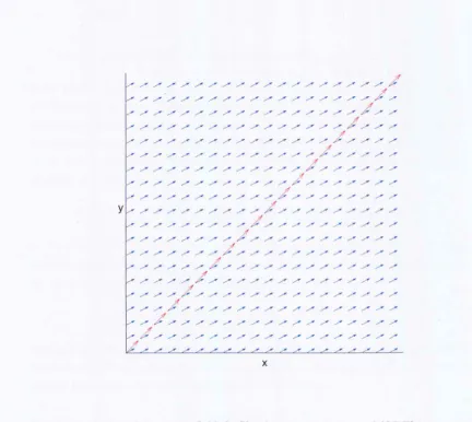
is a suitable weak solution of the 3D Navier-Stokes equations.

2.1.5 A flow into a Cantor set .

In this section we construct the map illustrated in Figure 2.2. The figure indicates

that under X the unit interval [0,1) is mapped at time t = 2 - 21_-j _{into the lh}

stage in the construction of the Cantor middl third set. After rigorously defining

X we demonstrate in Lemma 2.28 that for each x E [0,1) as t -7 T the trajectory

X

C

t

,

x) converges to a point in the Cantor set. Consequently; X does not preserve the Hausdorff or box-counting dimensions of the unit interval.

Further, in L mma 2.29 we demonstrate that X is sufficiently regular to give rise to a classical flow solution and in Lemma 2.30 we demonstrate that the

trajectories of X do not intersect.

-8/9

--7/9

- --====

-==-=-2/3

Q)

<J ro 1/2

a.

en

1/3 2/9

1/9

---

~

0

0 3/2 7/4

Time

Figure 2.2: The maps t 1-7 X (t, x) plotted up to time t =

i

for various initial data x E [0,1).

First, we recall that the jth stage of the Cantor middle third set is the

set of intervals C_i:= Up P

j

[p

,

P

+

3

-j₊1_{] where the set of left end points of these}

intervals

P.

i

is d fined inductively by P1:= {O} and PH 1:= (2 . 3j Pj) UPj. We write

Qj:= P_j+3-H 1 _{for the set of right end point of the intervals C j. The Cantor middle}

[image:33.549.43.517.83.773.2]

Define the map Y1 : [0,1] x [0,1) ----t [0,1) by

illustrated in Figure 2.3.

Q)

u

2/3

~ 1/2

(f)

1/3

-

---

---:::..::::....

---=-=--O :Sx<~

1

"2:Sx < l

o L---~---~

o

Time

Figure 2.3: Th maps t H Y1 (t,x) for various initial data x E [0,1).

Observe that at time t

=

1

Y1(1,x)=

{

~x

_3·

~x

+

1

3 3

o :S x < ~ ~ :S x < l

(2.10)

and in particular the images of the intervals [O,~) and [~, 1) under th map Y at

time t = 1 are Y1 (I, [0, ~)) = [0,1) and Y1

(1

,

[~, 1)) = [~, 1) respectively. More

concisely, we write

(2.11)

so that the range of Y₁ at time t = 1 is contained in the second stage of construction

of the Cantor middle third set C2 . By rescaling, duplicating and translating the

[image:34.549.68.511.22.679.2]

in later stages C{

define the map Y2: [1,1

+

~] X C2 \ Q2

-+

[0,1) by

{

Yl (2t - 2, 3x) /3

°

:;

x

<

~

Y2 (t;,x) := 2 2 2

Yd

2t - 2,3

(

x -

3)) /3

+

3 3:;

x

<

1,

which can be thought of as two translated copi s of the map Y1 rescaled temporally by a factor of 2 and patially by a factor of 3, illustrated in Figure 2.4. Observe

that 2/3

~ ~ 1/2

(/)

1/3

--~

---:-..:::::=

::----==

oL---~---~---~

o 3/2

Time

Figure 2.4: The maps t r--t Y2 (t,x) for various initial data x E [0,1).

Y2 (1

+

~

,

Y1 (1, [0, 1))) = Y2 (1

+

~

,C2

\ Q2) = C3 \ Q3·

For all j EN with j

2:

2 we define tj := 2- 2-(j-l) and the map

YJ:

[tj-l, tjl x

Cj \ Qj

-+

[0,1) by

{

YJ

-

l

(2t - 2, 3:r;) /3

Yj (t,x) := 2 2

YJ

-1 (2t - 2, 3

(

x -

3)) /3

+

3

o :; x < ~

~ :; x < l, (2.12)

Observe that for all j E N

Next, we let T:= limj-too tj = 2 and assemble the maps Yj in the following way: let the map X: [0, T) x [0,1)

--+

[0,1) be defined by

X (t,x) := {

Ydt, x) 0::; t ::; 1

Yj (t, X (tj-I, x)) tj-I

<

t ::; tj (2.13)

so that under the action of X each x E [0, 1) is sent via the map Y_I to a point in

C2 \ Q2 at time

t

= 1. Subsequently, this point is sent via the map Y2 to a point in

C3 \ Q3 at time t = 1

+

~, as illustrated in Figure 2.2. This continues for all j E N as

t

--+

T.

Lemma 2.27. Let the map X be as defined in (2.13). For ali x E [0,1) the map t H X (t, x) is continuously differentiable on

[0,

T).

Proof. Observe from the definition (2.10) for all x E [0,1) the map t H YI (t, x) is continuously differentiable o~ (0,1). It follows that for all with j

2

2 and for each x E Cj \ Qj the map t H Yj (t,x) is continuously differentiable on (tj-I,tj). Consequently, for each x E [0, 1) the map t H X (t, x) is continuously differentiable on the open interval (tj-I, tj) for each j. Further, the continuity of t H X (t, x) at tj-I for each j follows immediately from the definition (2.13).

It remains to show that

t

H X

(t,

x) is continuously differentiable at each tj-I. From (2.10) it is apparent that

aYI (0 )

=

aYI (1 x)

=

°

V x E [0,1)

at ,x at '

and so, as the Yj are rescaled YI, for each j

2

2

ay.

ay.

a: (tj-I,X) = a: (tj, x) =

°

V x E Cj \ Qj.

Consequently, the derivatives of

t

H X

(t,

x) from above and below at tj-I are equal

to zero, so

¥t

exists and is continuous at tj-I. 0 Next, we extend X to the closed time interval [0, TJ.

Proof. It is immediate from the definition of Yl that

YI(t,x) E [0,1) VtE [0,1) V;XE [0,1).

Consequently, as the Yj consists of rescaled copies of the map Yl , for all j 2=: 2

Consequently, for each fixed x E [0, 1)

As t H X (t, x) is continuous on [0, T) as t

-+

T the map X (t, x) takes values in nested intervals whose length tends to zero, so X

(t,

x) converges as

t

-+

T. 0

We define the map

X:

[0,

T]

x [0, 1)

-+

[0, 1) by

_ {X(t,X) tE[O,T)

X (t,x) :=

limt-+T X (t, x) t = T.

(2.14)

Lemma 2.29. Let the map

X

be as defined in (2.14). For each x E

[0,

1) t~e map t H

X

(t, x) is continuously differentiable on the closed interval

[0,

T].

Proof. In light of Lemma 2.27 it is sufficient to demonstrate that X is continuously differentiable at t

=

T. Clearly, from (2.14), t H X (t,x) is continuous at t

=

T. Further, from the definition (2.10), the derivative

and it is straightforward to show that

l

aY

l

I

_{1 ]}

at (t,x) :::;

4

Vt E [0,1 ,

o:::;x<!

!:::;x<l

v

x E [0,1). (2.15) Further, from the definition (2.12), for all t E [tj-l, tj] and all x E Cj \ Qj the derivative

_ J (t x) =

l

aYI

{2a~tl

(2t-2,3x)/3

a t ' 2a~tl (2t - 2,3 (x - ~)) /3

+

~