Original citation:
Sprittles, James E.. (2015) Air entrainment in dynamic wetting: Knudsen effects and the
influence of ambient air pressure. Journal of Fluid Mechanics, 769 . pp. 444-481.
Permanent WRAP URL:
http://wrap.warwick.ac.uk/78923
Copyright and reuse:
The Warwick Research Archive Portal (WRAP) makes this work by researchers of the
University of Warwick available open access under the following conditions. Copyright ©
and all moral rights to the version of the paper presented here belong to the individual
author(s) and/or other copyright owners. To the extent reasonable and practicable the
material made available in WRAP has been checked for eligibility before being made
available.
Copies of full items can be used for personal research or study, educational, or not-for profit
purposes without prior permission or charge. Provided that the authors, title and full
bibliographic details are credited, a hyperlink and/or URL is given for the original metadata
page and the content is not changed in any way.
Publisher’s statement:
© 2015 Cambridge University Press.
http://dx.doi.org/10.1017/jfm.2015.121
A note on versions:
The version presented here may differ from the published version or, version of record, if
you wish to cite this item you are advised to consult the publisher’s version. Please see the
‘permanent WRAP url’ above for details on accessing the published version and note that
access may require a subscription
Air Entrainment in Dynamic Wetting: Knudsen Effects and the
Influence of Ambient Air Pressure
James E. Sprittles
Mathematics Institute, University of Warwick, Coventry, CV4 7AL, UK
March 3, 2015
Abstract
Recent experiments on coating flows and liquid drop impact both demonstrate that wetting failures caused by air entrainment can be suppressed by reducing the ambient gas pressure. Here, it is shown that non-equilibrium effects in the gas can account for this behaviour, with ambient pressure reductions increas-ing the gas’ mean free path and hence the Knudsen number Kn. These effects first manifest themselves through Maxwell slip at the gas’ boundaries so that for sufficiently smallKnthey can be incorporated into a continuum model for dynamic wetting flows. The resulting mathematical model contains flow structures on the nano-, micro- and milli-metre scales and is implemented into a computational platform developed specifically for such multiscale phenomena. The coating flow geometry is used to show that for a fixed gas-liquid-solid system (a) the increased Maxwell slip at reduced pressures can substantially delay air en-trainment, i.e. increase the ‘maximum speed of wetting’, (b) unbounded maximum speeds are obtained as the pressure is reduced only when slip at the gas-liquid interface is allowed for and (c) the observed be-haviour can be rationalised by studying the dynamics of the gas film in front of the moving contact line. A direct comparison to experimental results obtained in the dip-coating process shows that the model recovers most trends but does not accurately predict some of the high viscosity data at reduced pressures. This discrepancy occurs because the gas flow enters the ‘transition regime’, so that more complex descriptions of its non-equilibrium nature are required. Finally, by collapsing onto a master curve experimental data obtained for drop impact in a reduced pressure gas, it is shown that the same physical mechanisms are also likely to govern splash suppression phenomena.
1
Introduction
The behaviour of liquid-solid-gas contact lines, at which an ambient gas is displaced by a liquid spreading over a solid, is the key element of many technological processes, ranging from coating flows used to apply thin liquid films to substrates (Weinstein & Ruschak, 2004) through to 3D printers being developed to economically produce bespoke geometrically-complex structures (Derby, 2010). Often, limitations on the operating devices are imposed by ‘wetting failure’ which occurs when the liquid can no longer completely displace the gas at the contact line. In coating technologies, this leads to the entrainment of gas bubbles into the liquid film which destroy its carefully tuned material properties whilst in drop-based flows entrainment of air under the moving contact line promotes the formation of splashes which, again, are usually undesirable. Consequently, understanding the physical mechanisms which control wetting failure and, where possible, delaying this occurrence by manipulating the material parameters, flow geometry, etc, to ever increasing wetting speeds is one of the key aims of research into dynamic wetting.
Recent experimental studies have discovered new ways in which to delay the onset of wetting failures. Specifically, in both coating flows (Benkreira & Khan, 2008; Benkreira & Ikin, 2010) and drop impact phenomena (Xu et al., 2005; Xu, 2007) it has been shown that a sufficient reduction in the pressure of the ambient gas, around a factor of ten in the former case and even less in the latter, can suppress wetting failures. This result was unexpected, as until Xuet al.(2005) it was assumed that the gas’ dynamics can either be entirely neglected or, as found in coating research, only influences the system’s behaviour through viscous forces which act in the thin gas film in front of the moving contact line (Kistler, 1993). However, the significance of the viscous forces in the gas is usually characterised by the viscosity ratio between the gas and the liquid, and this remains unchanged by variations in gas pressure. Why then, would reductions in ambient pressure have any influence on the contact line’s dynamics?
An interpretation of the aforementioned phenomena, suggested in a number of different contexts, is that the reduction in ambient gas pressure, which leads to a corresponding decrease in gas density, increases the mean free path in this phase so that non-equilibrium gas dynamics (Chapman & Cowling, 1970), also referred
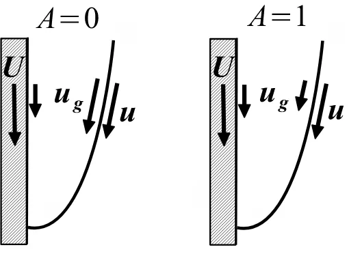
Figure 1: Sketch illustrating the influence of gas flow on the drop impact phenomenon. The behaviour of the gas, in the regions indicated by block arrows, affects both (a) the pre-impact and (b) the post-impact spreading dynamics of the drop.
to as rarefied gas dynamics (Cercignani, 2000), become important (Marchand et al., 2012; Benkreira & Ikin, 2010; Duchemin & Josserand, 2012). Specifically, boundary slip is generated in the gas whose magnitude is proportional to the mean free path and thus whose influence is increased by reductions in gas pressure. The increased slip allows gas trapped in thin films between the solid and the free-surface to escape more easily, so that the lubrication forces generated by the gas are reduced and its influence is negated.
For drop impact phenomena, whose literature has been previously reviewed (Rein, 1993; Yarin, 2006), alterations in the lubrication forces could be important either (a) in the thin air cushion that exists under the drop before it impacts the solid (Bouwhuis et al., 2012; Thoroddsen et al., 2005) and/or (b) in the gas film formed in front of the advancing contact lineafter the drop has impacted the solid (Riboux & Gordillo, 2014), see Figure 1. Theoretical work has also focussed on either (a) the pre-impact stage (Smithet al., 2003; Mani
et al., 2010; Mandre & Brenner, 2012) or (b) the post-impact spreading phase where, with a few exceptions (Schrollet al., 2010), the gas is usually considered passive (Bussmannet al., 2000; Eggerset al., 2010; Sprittles & Shikhmurzaev, 2012a). Distinguishing how each of these processes influences the spreading dynamics of the drop is a complex problem, both from a theoretical and experimental perspective, due to the inherently multiscale nature of the phenomenon. As a result, establishing how reductions in ambient pressure suppress splashing remains an area of intensive debate (Driscoll & Nagel, 2011; Kolinskiet al., 2012; de Ruiteret al., 2012) with recent experimental results on the impact stage particularly interesting (de Ruiteret al., 2015; Kolinskiet al., 2014).
In contrast to drop-based dynamics, for the dip-coating flow investigated in Benkreira & Khan (2008) mechanism (a) does not exist, as up until the point of wetting failure, the liquid remains in contact with the solid and the motion is steady. Therefore, studying this process allows us to isolate the influence of changes in ambient pressure on the behaviour of a moving contact line, i.e. effect (b), without any of the aforementioned complications that are inherent to the drop impact phenomenon. This is the path that will be pursued in this work with drop dynamics only re-considered again in§7 where, having characterised fully (b), our results enable us to infer some conclusions about drop splashing phenomena.
1.1
Experimental Observations in Dip Coating
The experimental setup constructed in Benkreira & Khan (2008) is for dip-coating, where a plate/tape is con-tinuously run through a liquid bath (Figure 2) and gradually increased in speed until air is entrained into the liquid. The speed at which this first occurs is called the ‘maximum speed of wetting’ and will be denoted byU?
c,
where stars will be used throughout to denote dimensional quantities. In contrast to previous works (Burley & Kennedy, 1976; Blake & Shikhmurzaev, 2002), the ambient gas pressure P?
g can be reduced from its
atmo-spheric value by up to a factor of a hundred by mounting this apparatus inside a vacuum chamber. Silicone oils of differing viscosities are used as the coating liquid, because their relatively low volatility (compared to, say, water-glycerol mixtures) ensures no significant evaporation when the ambient pressure is reduced. This work is extended in Benkreira & Ikin (2010) to consider also a range of different ambient gases (air, carbon dioxide and helium). The key results from Benkreira & Khan (2008) can be summarised as follows:
• For a given liquid-solid-gas system,U?
Figure 2: Sketch of the dip-coating flow configuration showing a free-surface formed between a liquid (below) and gas (above) which meets a solid surface at a contact line, which is a distance4y below the height of the surface (y = 0). The inset shows that the free-surface meets the solid at a contact angleθd but that a finite
distance away has an apparent angleθM at an inflection point in the surface profile where the film has height
H.
• There is very little variation in Uc? until Pg? is approximately a tenth of its atmospheric value. Further
reductions inPg? lead to sharp increases inUc?. • For sufficiently low P?
g, it is possible for high viscosity liquids to have a larger value of Uc? than lower
viscosity ones (the opposite of what occurs at atmospheric pressure).
In addition to these findings, in Benkreira & Ikin (2010) it is shown that:
• For a given value ofPg?, using a gas with a larger mean free path increasesUc?.
In Benkreira & Ikin (2010), the aforementioned experimental observations are assumed to be caused by non-equilibrium effects in the gas which become significant at sufficiently low pressures. These effects, most notably slip at the gas film’s boundaries, are interpreted in terms of an ‘effective gas viscosity’ whose magnitude is reduced with decreases in ambient gas pressure. Using appropriate values for this parameter, obtained from measurements of the resistance of a gas trapped between parallel oscillating plates (Andrews & Harris, 1995), allows the data to be collapsed onto a single curve (Figure 9b in Benkreira & Ikin (2010)) and highlights the influence of non-equilibrium effects.
Although the effective viscosity may be a useful concept when trying to qualitatively interpret the experi-mental findings, as anintegral property of the system it will not enable us to formulate alocal fluid mechanical model for this problem. In particular, the dependence of the effective gas viscosity on ambient gas pressure which is used in Benkreira & Ikin (2010) was obtained in Andrews & Harris (1995) for a gas film of constant height 2µm and will be different for other film profiles. In reality, the gas film’s height will vary all the way from the contact line to the far field, where a film can no longer be defined so that the notion of an effective viscosity no longer makes sense. Instead, we must look to capture the local physical mechanisms which alter the gas film’s dynamics at reduced pressures.
1.2
Mathematical Modelling of Dynamic Wetting Phenomena
Consider the various levels of description that can be used to describe dynamic wetting phenomena depending on how the gas phase’s dynamics are accounted for, with the simplest case first.
1.2.1 Dynamic Wetting in a Passive Gas
mechanical model, with no-slip at fluid-solid boundaries, has no solution (Huh & Scriven, 1971; Shikhmurzaev, 2006). This is the so-called ‘moving contact line problem’. And, secondly, the contact angle, which is seen to vary at experimental resolutions (Hoffman, 1975; Blake & Shikhmurzaev, 2002), must be prescribed as a boundary condition on the free-surface shape. A review of the various classes of models proposed to address these issues can be found in Ch. 3 of Shikhmurzaev (2007).
To overcome the moving contact line problem, initially identified in Huh & Scriven (1971), it is often assumed that some degree of slip occurs at the fluid-solid boundary (Dussan V, 1976). Methods for predicting the ‘slip length’ of an arbitrary liquid-solid interface are not well developed but estimates suggest it is in the range 1–10 nm for simple liquids (Laugaet al., 2007).
The treatment of the dynamic contact angle remains a highly contentious issue. The main question is whether or not the experimentally observed variation in the ‘apparent angle’ (Wilson et al., 2006) is caused entirely by the bending of the free surface below the resolution of the experiment, i.e. by the ‘viscous bending’ mechanism quantified in Cox (1986) and measured in Dussan Vet al.(1991); Ram´e & Garoff (1996), or whether actual contact angle (sometimes referred to as the ‘microscopic angle’) also varies. In either case, the apparent angle depends on the capillary number, which is the dimensionless contact line speed, but in the former case the actual angle remains fixed whilst in the latter this angle varies, as in the molecular kinetic theory (Blake & Haynes, 1969). In more complex models, the angle can also depend on the flow field itself, as in the interface formation model (Shikhmurzaev, 2007).
Models in which the contact angle is considered constant have been popular in recent years for investigating air entrainment phenomena and have produced a number of promising results (Vandreet al., 2012, 2013, 2014; Marchandet al., 2012; Chan et al., 2013). What is clear from simulations is that viscous bending of the free surface becomes significant as the point of air entrainment is approached and cannot be neglected. What remains unclear is whether this mechanism is sufficient to account for the experimentally observed dynamics of the apparent contact angle, particularly given that precise measurements of the magnitude of slip on the liquid-solid interface are lacking. These difficulties have stimulated fundamental research into the contact line region’s dynamics using molecular dynamics techniques (De Coninck & Blake, 2008) but, as can be seen from a recent collection of papers (Velarde, 2011) and review articles (Blake, 2006; Snoeijer & Andreotti, 2013), intense debate remains about the topic.
The focus of this work is to characterise the effects which the gas dynamics can have on dynamic wetting phenomena and, consequently, the simplest possible model for the other aspects will be used. Specifically, slip at the liquid-solid interface will be captured using the Navier condition (Navier, 1823), as commonly used in dynamic wetting models (Hocking, 1976; Huh & Mason, 1977), and the contact angle will be taken as a parameter that is fixed at its equilibrium value. The result is a ‘conventional model’ and a comprehensive review of all such models which can be ‘built’ is given in Ch. 9 of Shikhmurzaev (1997). More complex models can easily be constructed on top of the model used here, but in the present context would distract from the main focus of this work.
1.2.2 In a Viscous Gas
It is now well recognised that at sufficiently high coating speeds a thin film of gas forms in front of the moving contact line, as observed experimentally by laser-Doppler velocimetry in Mueset al. (1989). The thin nature of the film means that despite the large viscosity ratio, lubrication forces enhance the influence of the gas’ dynamics so that they cannot be neglected. As coating speeds are increased, the resistance this film creates to contact line motion eventually becomes sufficiently large that it is entrained into the liquid (Vandre et al., 2013; Marchandet al., 2012). Therefore, to study the phenomenon of air entrainment and wetting failures, any theory developed must account for the dynamics of the viscous gas as well as the liquid.
In formulating a model for the gas’ dynamics one again encounters the moving contact line problem, namely that if no-slip is used then the contact line can’t move. Consequently, slip has also often been applied on the solid-gas boundary with a magnitude, measured by the slip length, either explicitly stated to be the same as in the liquid (Vandreet al., 2013) or implicitly assumed to be so (Cox, 1986). In other words, slip is usually used as a mathematical fix to circumvent the moving contact line problem, rather than as a physical effect whose magnitude can significantly alter the flow.
1.2.3 In a Non-Equilibrium Gas
Experimental observations in Marchandet al.(2012), where the film entrained by a plunging plate was measured using optical methods, suggest that for relatively viscous liquids the characteristic film thickness is rather small, in the range H? ∼1–15µm. For flows where there is an external load on the film, such as in curtain coating,
the film’s thickness is likely to be even smaller. Consequently, the film’s dimensions become comparable to the mean free path in the gas `? so that the Knudsen number Kn
H = `?/H?, characterising the importance of
Figure 3: The effect of Maxwell-slip on the gas flow. WhenA= 0 slip is present at the gas-solid boundary but turned off at the gas-liquid boundary, so thatug=ug, whilst forA= 1 it is present on both interfaces.
ten decrease in the ambient pressure of air, achieved in both Benkreira & Khan (2008) and Xu et al.(2005), gives a value of`?= 0.7 µm so that Kn
H ∼0.1. In this case, one may expect that non-equilibrium effects in
the gas film will have a significant impact on its dynamics, and we must consider how this can be incorporated into our dynamic wetting model.
Non-equilibrium effects first manifest themselves at the gas’ boundaries and can be accounted for by relaxing the no-slip condition to allow for boundary slip whilst continuing to use the the Navier-Stokes equations in the bulk. This approach remains accurate for KnH <0.1, during which gas flow is said to be in the ‘slip regime’,
after which Knudsen layers will begin to occupy the entire gas film, so that the scale separation between boundary and bulk effects no longer exists.
In Maxwell (1879), a slip condition was derived for the ‘micro-slip’ at the actual boundary of the gas whose mathematical form remains the same, when KnH 1, if ‘macro-slip’ across a Knudsen layer of size ∼`? is
also accounted for, see§3.5 of Cercignani (2000). We shall henceforth refer to the discontinuity in tangential velocity as ‘Maxwell slip’ which at an impermeable boundary is generated by the stress acting on that interface from the gas phase. For two-dimensional isothermal flow, the component of velocityu?g, where subscriptsg will
denote properties of the gas, adjacent to a stationary planar surface located aty= 0 is, in dimensional terms, given by:
a `? ∂ u
? g
∂y? =u ?
g (1)
where the coefficient of proportionality a can depend on both the properties of the micro-slip, which will depend on the fraction of molecules which reflect diffusively and those which a purely specular, and the macro-slip generated across a Knudsen layer. In practise, unless surfaces are molecularly smooth we will havea∼1 (Agarwal & Prabhu, 2008; Millikan, 1923; Allen & Raabe, 1982) and, for simplicity, we will henceforth take
a= 1.
The Maxwell slip condition (1) has the same form as the slip conditions which have often been used in dynamic wetting flows to circumvent the moving contact line problem in the gas but occurs naturally here from the consideration of non-equilibrium gas effects. Notably, this means that accurate values of the slip length can easily be obtained by knowing the mean free path in the gas, in contrast to the slip length in the liquid which is notoriously difficult to determine. Furthermore, the approach taken here suggests that slip will also be present at the gas-liquid boundary (i.e. the free-surface), as demonstrated by experiments dating back to Millikan (1923). This effect is shown in Figure 3, where the parameterA is used to change between the usual condition of continuity of velocity across the gas-liquid interface (A= 0) and Maxwell-slip (A= 1).
Slip at the gas-liquid boundary has been accounted for in some models for the gas film in drop impact (Duchemin & Josserand, 2012; Maniet al., 2010), and in great detail for drop collisions (Sundararajakumar & Koch, 1996), but is yet to be routinely incorporated into dynamic wetting models. In most cases where slip on the gas-solid interface is accounted for, the same effect on the gas-liquid surface is not considered (Vandre
et al., 2013; Riboux & Gordillo, 2014). The only progress in this direction has been achieved in Marchand
In order to apply Maxwell-slip at curved moving surfaces, the tensorial expression is required (Lockerby
et al., 2004). Specifically, for gas flow adjacent to a surface which moves with velocity u? and has normal n
pointing into the gas, we have
`? n· ∇u?g+ [∇u?g]T
·(I−nn) =u?g||−u?||, (2) where the subscriptsk denote the components of a vector tangential to the surface which can be obtained for an arbitrary vectora usinga||=a·(I−nn), whereIis the metric tensor of the coordinate system.
If the gas is modelled as being composed of ‘hard spheres’, then the mean free path is related to the temperatureT? and ambient pressureP?
g by`?=k?BT?/( √
2πP?
g(l?mol)2) where l?mol is the molecular diameter
andk?
B is Boltzmann’s constant. Notably, if local variations in gas pressure about Pg? are small, which will be
the case here, then for a given ambient pressure`? is fixed throughout the entire gas phase. In practise, when
considering the dependence of the mean free path of a gas on the ambient pressure at a fixed temperature it is convenient to use the expression
¯
`≡ ` ?
`? atm
= P
? g,atm
P? g
≡1/P¯g (3)
where ¯Pgis the gas pressure normalised by its atmospheric value. At atmospheric pressure, air has a mean free
path`?atm= 0.07µm and other commonly encountered gases take similar values`?atm∼0.1 µm.
Although the Knudsen number in the gas film KnH is of most interest, this can only be obtained once our
computations have allowed us to findH?. Before then, the Knudsen number based on our characteristic scales
Kn=`?/L?, whereL?∼1 mm is the capillary length, must be used. Noting that the dimensionless mean free
path at atmospheric pressure is`atm=`?atm/L?, the resulting expression forKntakes the form
Kn=`atm¯
Pg
(4)
so that the explicit dependence on pressure reduction becomes clear.
1.3
Overview
This work will answer the following questions:
• Can increases in Maxwell slip, caused by experimentally-attainable reductions in ambient gas pressure, significantly raise the maximum speed of wetting?
• Does slip on the liquid-gas interface, usually neglected in this class of flows, have a substantial effect on the dynamic wetting process?
• Will the magnitude of the Knudsen number based on the gas film’s height KnH be small enough for the
gas flow to remain in the ‘slip regime’ ?
• Is it possible to collapse the data from Xu et al. (2005) onto a master curve by assuming that non-equilibrium gas effects are responsible for splash suppression in drop impact?
2
Problem Formulation
Consider the flow generated by the steady motion of a smooth chemically-homogeneous solid surface which is driven through a liquid-gas free surface in a direction aligned with gravity at a constant speedU?(see Figure 2).
A characteristic length scale for this problem is given by the capillary length L? = qσ?/((ρ?−ρ? g)g?) '
p
σ?/(ρ?g?), where σ? is the surface tension of the liquid-gas surface, which is assumed constant; g? is the
acceleration due to gravity; andρ?, ρ?
g are the densities in the liquid and gas, respectively, withρ?g/ρ? 1 in
the liquid-gas systems of interest so that the capillary length can be determined solely from the liquid’s density. A scale for pressure isµ?U?/L?, where µ? is the viscosity of the liquid andµ?
g will be its value in the gas.
2.1
Bulk equations
For compressibility effects in the liquid and gas to be negligible we require that the Mach numberM a=U?/c?
in each phase remains small, wherec? is the speed of sound. Given thatU?<1 ms−1andc?>100 ms−1in all
cases considered, we have M a <0.01. However, this is not a sufficient condition for the flow to be considered incompressible, especially when there are thin films of gas present along which pressure can vary significantly, see §4.5 of Gad-el-Hak (2006). Here, we will assume that the flow in both phases can be described by the steady incompressible Navier-Stokes equations and in §4.5 the validity of this assumption will be confirmed from a-posteriori calculations. Therefore, we have
∇ ·u= 0, Cau· ∇u=Oh2(∇ ·P+ ˆg/Ca), (5)
∇ ·ug= 0, ρ Ca¯ ug· ∇ug=Oh2(∇ ·Pg+ ¯ρg/Caˆ ), (6)
where the stress tensors in the liquid and gas are, respectively,
P=−pI+h∇u+ (∇u)Ti and Pg =−pgI+ ¯µ
h
∇ug+ (∇ug) Ti
. (7)
Here, uandug are the velocities in the liquid and gas;pand pg are the local pressures in the liquid and gas,
in contrast to uppercaseP’s which are used for the ambient pressure in the gas;Ca=µ?U?/σ? is the capillary
number based on the viscosity of the liquid; the viscosity ratio is ¯µ=µ?
g/µ?; the ratio of gas to liquid densities is
¯
ρ=ρ?g/ρ?; and ˆgis a unit vector aligned with the gravitational field. The Ohnesorge numberOh=µ?/√ρ?σ?L?
has been chosen as a dimensionless parameter, instead of the Reynolds numberRe=Ca/Oh2=ρ?U?L?/µ?, as for a given liquid-solid-gas combinationOhwill remain constant, i.e. it will depend solely on material parameters and be independent of contact-line speed.
2.2
Boundary Conditions at the Gas-Solid Surface
Conditions of impermeability and Maxwell slip give
ug·ns= 0, Knns·Pg·(I−nsns) =ugk−Uk, (8)
whereUis the velocity of the solid and the normal to the solid surface is denoted as ns.
2.3
Boundary Conditions at the Liquid-Gas Free-Surface
On the free-surface, whose location must be obtained as part of the solution, for a steady flow the kinematic equation and continuity of the normal component of velocity give that
u·n=ug·n= 0, (9)
where n is the normal to the surface pointing into the liquid phase. These equations are combined with the standard balance of stresses with capillarity that give
n·(P−Pg)·(I−nn) =0, n·(P−Pg)·n=∇ ·n/Ca. (10)
Equations (9) and (10) are usually combined with a condition stating that the velocity tangential to the interface is continuous across itugk=uk. However, when Maxwell slip is accounted for this is replaced with
−A Knn·Pg·(I−nn) =ugk−uk, (11)
2.4
Boundary Conditions at the Liquid-Solid Surface
The standard conditions of impermeability and Navier slip give
u·ns= 0, lsn·P·(I−nsns) =uk−Uk, (12)
where ls = ls?/L? is the dimensionless slip length based on the (dimensional) slip length at the liquid-solid
interfacel?
s. This parameter has no relation to the slip coefficient in the gas which was based on the mean free
path`?. In other words, although Maxwell slip and Navier slip have the same mathematical form, their physical
origins differ and thus there is no reason to expect their coefficients to have similar magnitudes.
2.5
Liquid-Solid-Gas Contact Line
Equation (10) requires a boundary condition at the contact line which is given by prescribing the contact angle
θd satisfying
n·ns=−cosθd. (13)
Here, our focus is on understanding the effects of the gas dynamics on the dynamic wetting flow so that we will take the simplest option of assumingθdto be a constant. More complex implementations, such as those in
Sprittles & Shikhmurzaev (2013), can be considered in future research.
2.6
‘Far Field’ Conditions
Dip coating is usually conducted in a tank of finite size whose dimensions are large enough not to alter the dynamics close to the contact line, as confirmed in Benkreira & Khan (2008). The influence of system geometry, or ‘confinement’, on the dynamic wetting process are well known (Ngan & Dussan V, 1982) and, in particular, have been used to delay air entrainment (Vandreet al., 2012), but these effects are not the focus of this work. Therefore, the ‘far field’ boundaries of our domain, which are assumed to be no-slip solidsu=ug =0, are set
sufficiently far from the contact line that they have no influence on the dynamic wetting process. Where the free-surface meets the far-field it is assumed to be perpendicular to the gravitational field, i.e. ‘flat’, so that
n·ˆg= 1. In practise, setting the far field (dimensionally) to be twenty capillary lengths from the contact line in both thexandy directions was found to be sufficiently remote.
3
Computational Framework
Dynamic wetting and dewetting flows have often been investigated using the simplifications afforded by the lubrication approximation (Voinov, 1976; Eggers, 2004). However, for the two phase flow considered here, this approximation cannot simultaneously be valid in each phase, i.e. the liquid and gas phases can’t both be thin films. As shown in recent papers (Marchandet al., 2012; Vandreet al., 2013), plausible extensions in the spirit of the lubrication approach can be attempted, but their accuracy can only be ascertained from comparisons to full computations and is unlikely to be acceptable at larger capillary numbers where the contact line region cannot be considered as ‘localised’.
At present, to obtain accurate solutions to the mathematical model formulated in §2, one is left with no option other than to use computational methods.
Computationally, resolving all scales in the problem is particularly important to ensure that our contact line equation (13) is applied to the ‘actual’ or ‘microscopic’ angleθd, rather than the ‘apparent one’θapp=θapp(s),
i.e. the angle of the free surface at a finite distances from the contact line. Although the apparent angle can, in certain circumstances, be related to the actual angle (Cox, 1986), this will not be true at the high capillary numbers observed in coating flows, particularly when non-standard gas dynamics are included.
Here, gas dynamics will be built into a finite element framework developed in Sprittles & Shikhmurzaev (2012c, 2013) to capture dynamic wetting problems and then extended to consider two-phase flow problems in our work on the coalescence of liquid drops (Sprittles & Shikhmurzaev, 2014b). Notably, this code captures all physically-relevant length scales in the problem, from the slip lengthl?s∼10 nm up to the capillary length
L? ∼ 1 mm, meaning that at least six orders of magnitude in spatial scale are resolved. As a step-by-step user-friendly guide to the implementation has been provided in Sprittles & Shikhmurzaev (2012c), only the main details will be recapitulated here alongside some aspects which are specific to the current work.
The mesh is graded so that small elements can be used near the moving contact line to resolve the slip length whilst larger elements are used where only scales associated with the bulk flow are present. Consequently, the computational cost is relatively low so that even for the highest resolution meshes used in this work, for a given liquid-solid-gas combination the entire map of, say,Cavs contact line elevation (4y), can be mapped in just a few hours on a standard laptop.
Computations at highCa, roughly those for whichCa >0.1, are notoriously difficult as (a) the free-surface becomes increasingly sensitive to the global flow and (b) regions of high curvature at the contact-line require spatial resolution on scales at or below the slip length ls. Both factors hinder the ease at which converged
solutions can be obtained and these issues are compounded when Oh is small, indicating the importance of non-linear inertial effects. For all parameter sets computed, converged solutions can always be obtained for
Ca≤2, which compares very favourably to previous works, so that this is chosen as an upper cut-off for the results of our parametric study.
3.1
Benchmark Calculations for the Maximum Speed of Wetting
In coating flows, one would like to know for a given liquid-solid-gas combination the wetting speed U? c at
which the contact line motion becomes unstable so that gas is entrained into the liquid either through bubbles forming at the cusps of a ‘sawtooth’ wetting-line (Blake & Ruschak, 1979) or by an entire film of gas being dragged into the liquid (Marchandet al., 2012). This is referred to as the ‘maximum speed of wetting’ and, in dimensionless terms, is represented by a critical capillary numberCac=µ?Uc?/σ?. Our method for calculating
Cac is explained in the Appendix alongside benchmark calculations for its value which are compared to the
results of Vandreet al.(2013) across a range of viscosity ratios. Excellent agreement is obtained between the results in Vandreet al.(2013) and those found here. As these calculations distract from the main emphasis of this work, but could be useful as a benchmark for future investigations in the field, they are provided in the Appendix.
4
Effect of Gas Pressure on the Maximum Speed of Wetting:
Anal-ysis of a Base State
Having demonstrated the accuracy of our code and shown how the critical capillary numberCac is calculated,
we now investigate the relation between the gas pressure ¯PgandCac. Here, we will analyse a base state, varying
only gas pressure and A, in an attempt to deepen our understanding of the influence of non-equilibrium gas effects on the dynamic wetting process before, in§5, performing a parametric study of the system of interest.
To ensure we are studying an experimentally attainable regime, we use the system considered in Benkreira & Khan (2008) to provide a base state about which our parameters can be varied. In this work, a range of silicone oils of different viscosities µ? = 20–200 mPa s are used whilst the densityρ? = 950 kg m−3, surface
tensionσ? = 20 mN m−1 and equilibrium contact angle θ
e = 10◦ remain approximately constant. Then the
characteristic (capillary) length L?= 1.5 mm andOh = 6×10⁻³µ? (mPa s)−1 depends only on the viscosity µ?.
A base case is chosen by taking µ?= 50 mPa s so thatOh0 = 0.3, where base state values will be denoted
with a subscript 0. Taking air as the displaced fluid with µ?
g = 18 µPa s, which remains independent of the
ambient pressure (Maxwell, 1867), gives a viscosity ratio of ¯µ0= 3.6×10⁻⁴. The density of the gasρ?
gdepends
on the ambient gas pressure, with its maximum value of ρ?
g = 1.2 kg m−3 at atmospheric pressure making
¯
ρmax= 1.3×10⁻³. However, for all calculations performed, the value of ¯ρhas a negligible effect onCac when
¯
ρ≤ρ¯max and so henceforth, without loss of generality, we take ¯ρ= 0.
The slip length of the liquid-solid interface is fixed at l?s = 10 nm, which is well within the range of
experimentally observed values (Lauga et al., 2007), so that the dimensionless parameter ls = 6.8×10⁻⁶.
Assuming the gas is air, we haveKn= 4.8×10⁻⁵/P¯gso that the only parameter which remains to be specified
isAcharacterising whether or not there is slip at the gas-liquid boundary.
4.1
Effect of Gas Pressure
In Figure 4, the effect onCac of reducing ¯Pg is computed forA= 0 andA= 1. In each case, for ¯Pg>0.1 there
is only a slight increase inCac from its base value of 0.47, which is independent ofA. For ¯Pg<0.1, dramatic
changes in Cac are observed, whose form depends on A, so that ¯Pg ≈ 0.1 appears to be the point at which
non-equilibrium effects become important.
Notably, as can be seen most clearly in the inset of Figure 4, for A = 0 as ¯Pg →0 we have Cac →0.64
whereas forA= 1 computations suggest thatCac→ ∞. In fact, in the latter case, once a critical pressure ¯Pg,c
is approached, Cac appears to increase without bound. For A= 1 this occurs at ¯Pg,c= 9×10⁻³; just above
0 0.2 0.4 0.6 0.8 1 0
0.5 1 1.5 2
0 0.01 0.02 0.03 0.04 0.05 0
0.5 1 1.5 2
C ac
C ac
¯
P
g ¯Pg
2
1
[image:11.595.174.419.61.232.2]1 2
Figure 4: The dependence of the critical capillary numberCac on the gas pressure ¯Pg, for our base parameters,
with curve 1: A= 0 (in black) and 2: A= 1 (in blue). The inset shows how curve 1 (A= 0) tends to a finite value ofCac as ¯Pg→0 whilst curve 2 appear to increase without bound.
It is impossible to show rigorously that Cac → ∞as ¯Pg →P¯g,c without either the computation of higher
values of Cac, which would allow some scaling to be inferred, or, ideally, the development of an analytic
framework for this problem. Unfortunately, in the former case (see §3) computational constraints permit us from reachingCac>2 whilst in the latter we are confined by the fact that all analytic development, in particular
those of Cox (1986), are only valid for smallCac. Despite this, the rapid increase ofCac as ¯Pg,c is approached
is striking andCac = 2 is still a large value in the context of dip-coating phenomena.
To summarise, it has been shown that when Maxwell slip is accounted for on both the solid and gas-liquid interfaces the maximum speed of wetting appears to be unbounded as the ambient pressure is reduced, whereas if slip on the latter surface is neglected (A = 0), the maximum speed remains finite. In other words, the error associated with neglecting Maxwell slip on the free-surface is extremely large at reduced pressures and appears to be infinite in the limit ¯Pg→0.
4.2
Flow Kinematics
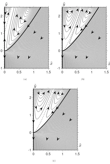
In Figure 5, streamlines of the flow near the contact line are shown atCa= 0.4 in three different regimes: (a) at a pressure where non-equilibrium effects are weak ¯Pg= 0.14 withA= 0, (b) ¯Pg= 0.14 withA= 1 and (c) at a
pressure where non-equilibrium effects are becoming influential ¯Pg= 0.014 withA= 1. Given thatL?∼ 1mm
for typical liquids, dimensionally the scale in Figure 5 is a few microns. In all cases, the flow of the liquid, which is below the free-surface (represented by a thick black line), remains virtually unchanged, with the motion of the solid, located at ˜x= 0, dragging liquid downwards which, to conserve mass, is continually replenished from above. If one notes that the free-surface meets the solid at an equilibrium contact angle of 10◦, and yet any apparent angle defined on the scale seen in Figure 5 would be obtuse, it is clear that at this relatively high capillary number there is significant deformation of the free-surface on a scale below what is visible here.
In all three cases, the flow of liquid, which seems immune to the gas’ dynamics, results in an almost identical velocity tangential to the free-surface on the liquid-facing side of this interface, as shown from curves 1a,2a,3a
in Figure 6a, where the velocities tangential to the gas-solid and liquid-gas interfaces have been plotted. At the top ˜y= 2.5 of the figures, the gas flow field is qualitatively similar in all cases. The motion of both the liquid and the solid drives gas towards the contact line region which, to ensure continuity of mass, results in a ‘split ejection’ type flow, as observed in immiscible liquid-liquid systems (Dussan V & Davis, 1974; Dussan V, 1977), with an upwards flux of gas through the middle of this domain. For A= 1 the split ejection flow is maintained right up to the contact line (Figure 5b,c); however, forA= 0 a flow reversal occurs on the solid-gas interface at ˜y ≈ 1 so that the direction of the gas flow actually opposes the solid’s for ˜y < 1 (Figure 5a). The flow reversal can clearly be seen from curve 1 in Figure 6b fors <10−3, with a substantial minimum of
u2t=−0.3, and can also be seen in previous works, such as Figure 10b of Vandreet al. (2013).
0
0.5
1
1.5
-1
0
1
2
˜
y
˜
x
(a)
0
0.5
1
1.5
-1
0
1
2
˜
y
˜
x
(b)
0
0.5
1
1.5
-1
0
1
2
˜
y
˜
x
[image:12.595.105.494.104.681.2](c)
Figure 5: Streamlines computed at Ca = 0.4 for different ambient gas pressures ¯Pg both with (A = 1) and
without (A= 0) Maxwell slip at the free-surface. In (a): ( ¯Pg, A) = (0.14,0), (b): (0.14,1) and (c): (0.014,1). The
local ‘zoomed in’ coordinates used are ˜x=x×103and ˜y= (y−yc)×103, whereycis the contact line position,
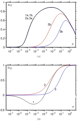
10−7 10−6 10−5 10−4 10−3 10−2 10−1 100 0
0.2 0.4 0.6 0.8 1
s
u
1t
1a,1b, 2a,3a
2b
3b
(a)
10−7 10−6 10−5 10−4 10−3 10−2 10−1 100 −0.5
0 0.5 1
u
2t
s
32
1
[image:13.595.171.422.193.586.2](b)
Figure 6: Tangential velocities as a function of distance from the contact linesalong the (a) liquid-gas and (b) gas-solid boundaries computed atCa= 0.4 with curve 1: ( ¯Pg, A) = (0.14,0), 2: (0.14,1) and 3: (0.014,1). The
velocity tangential to the free-surface and pointing towards the contact line is u1t, with subscripts ‘a’ for the
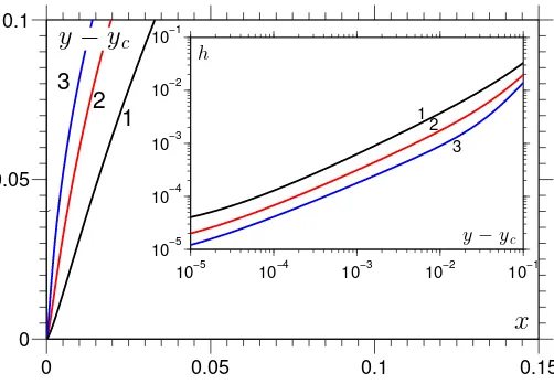
0 0.05 0.1 0.15 0
0.05 0.1
10−5 10−4 10−3 10−2 10−1
10−5 10−4 10−3 10−2 10−1
h
y−yc 1
3 2
y
−
y
cx
2 1
[image:14.595.170.421.61.235.2]3
Figure 7: Free-surface shapes obtained in our base case, with ¯Pg = 0.014, with curve 1: Ca= 0.4 (in black),
2: Ca= 0.6 (in red) and 3: Ca= 0.8 (in blue). The inset shows how the height of the gas filmhvaries as a function ofy−yc showing that for 10−4< y−yc<10−1 it can be considered in a lubrication setting.
When A= 1, slip is also allowed at the gas-liquid interface, see curves 2aand 2b in Figure 6a, so that, as can be seen from curve 2 in Figure 6b, there is no flow reversal on either of the gas’ boundaries. This more symmetric flow field remains when the gas pressure is decreased to ¯Pg= 0.014, see Figure 5c and curves labelled
3 in Figure 6. Although the flow remains qualitatively the same, one can clearly see from Figure 6 that lowering the pressure significantly increases slip at the gas’ boundaries. For example, at s= 10−2, for ¯Pg = 0.14 the
velocity on the solid u2t = 0.65 whereas for ¯Pg = 0.014 the velocity is just u2t= 0.16. Therefore, less gas is
dragged into the contact line region when (a) slip is accounted for on the gas-liquid boundary (A= 1) and/or (b) slip is increased through reductions in pressure. Both of these mechanisms reduce the gas’ resistance to contact line motion, as shown analytically in§4.4, and contribute to postponing the point of wetting failure.
4.3
Characteristics of the Gas Film
At high capillary numbers there is a region between the contact line and the far field in which the gas domain is a ‘thin film’. This region is sufficiently far from the contact line region where the free-surface bends from its equilibrium angle of 10◦towards an obtuse apparent angle and near enough to the contact line that gravitational forces have not started to flatten the free-surface. For our base case, for Ca≥ 0.4, which includes all values of Cac, this region exists between 10−4< y−yc <10−1 as one can see from Figure 7. Specifically, the main
figure clearly shows that the gas film is ‘thin’ on the scale of around y−yc ∼0.1 whilst the inset shows on a
logarithmic plot that this behaviour continues down toy−yc ∼10−4.
The dynamics of the gas film are key to the air entrainment phenomenon so that one may expect that reductions in ambient pressure will only start to influence Cac once Maxwell slip on the boundaries is large
enough to affect the gas’ flow characteristics. This happens when the (dimensionless) slip lengthKn= 4.8×
10−5/P¯gbecomes comparable to the height of the gas filmx=h(y). This results in afunctionKnloc(h) =Kn/h
which characterises the importance of non-equilibrium effects as one goes along the film. How though, should we define a particular position along the filmh=H on which we can base a local Knudsennumber KnH?
Research into dynamic wetting/dewetting phenomena (Dejaguin & Levi, 1964; Vandre et al., 2013; Eggers, 2004) has long recognised that wetting failure is strongly linked to the behaviour of the inflection point on the free-surface, where the surface’s curvature changes sign; this point can also be used to define an apparent contact angle (Tanner, 1979). Given that the flow near the inflection point seems to be key to determiningCac,
this point is a sensible choice for defining the characteristic film height H, see Figure 2. To do so, we must extractH from our computations and determine how it depends onCaand ¯Pg.
In Figure 8, we can see that although Cac depends on ¯Pg, the value ofH is approximately independent of
¯
Pg, so thatH ≈H(Ca), with smaller ¯Pgsimply revealing more of this curve. In fact, a similar curve is obtained
if the gas flow is ignored altogether (¯µ= 0), as shown by the dashed line in Figure 8, although this may not be the case at higher viscosity ratios. Notably,H decreases rapidly with increasingCain agreement with previous experiments (Marchandet al., 2012) and simulations (Vandreet al., 2013). Reassuringly, atCa=Cac the film
height obtained at atmospheric pressure,H = 4.2×10⁻³, dimensionally corresponds to a filmH? = 1–10µm
for typical liquids, which is precisely what has been found experimentally in Marchandet al. (2012).
Enhancements in Cac at reduced pressure can be quantified by the percentage increase in Cac from its
0 0.25 0.5 0.75 1 1.25 1.5 1.75 2 10−5
10−4 10−3 10−2 10−1
H
C a
1
2
[image:15.595.168.423.60.234.2]3
Figure 8: The dependence of the gas film heightH, at the inflection point on the free surface, on the capillary number Ca. The curve is largely independent of gas pressure ¯Pg, although the lower values of ¯Pg allow more
of the curve to be obtained. Curves corresponds to 1: ¯Pg= 1 (red), 2: ¯Pg = 10−2 (blue) and 3: ¯Pg = 9×10⁻³
(green), with the dashed line obtained for ¯µ= 0. .
4Cac P¯g H KnH
0 1 4.2×10⁻³ 0.011 10% 0.16 3.1×10⁻³ 0.1 20% 7×10⁻² 2.3×10⁻³ 0.3 50% 2.3×10⁻² 1.1×10⁻³ 1.9 100% 1.2×10⁻² 4.1×10⁻⁴ 9.8
≥300% ≤9×10⁻³ ≤7.1×10⁻⁵ ≥75
Table 1: The pressure reduction ¯Pg required for a given enhancement in capillary number 4Cac with the
corresponding film heightH and Knudsen number at the inflection pointKnH at this pressure.
as listing the pressure reduction required, values forH are given from whichKnH=Kn/H is calculated. The
data shows that for ¯Pg ∼0.1, where significant increases in4Cacbegin, corresponds toKnH∼0.1. Therefore,
non-equilibrium effects in the gas, which manifest themselves through Maxwell slip, alter the flow once the slip length is around 10% of the gas film’s characteristic height and it is this mechanism which determines when variations in ¯Pg can start to affectCac.
Notably, all inflection points calculated in Table 1 fall into the thin film region apart from the entries where the critical gas pressure has been passed after which the inflection point gets close to the region of high curvature near the contact line. This suggests that the critical pressure ¯Pg,c = 9×10⁻³ is the one which is low enough
for the inflection point to no longer be located the thin film region. From Table 1 we can see that for ¯Pg≤P¯g,c
we have KnH ≥75 so that Maxwell slip is so strong that the gas flow is hardly affected by the motion of its
boundaries. In this case, the gas effectively offers no resistance to the dynamic wetting process andCac is able
to increase without bound.
4.3.1 Limitations of the Maxwell-slip Model
From Table 1 it is clear that the combined increases in Kn and decreases in H at reduced pressures both contribute to rapid changes inKnH. Across a reduction in the gas pressure of∼102,KnH increases from its
atmospheric value by a factor of ∼104. Consequently, most values ofKnH in the Table fall well outside the
‘slip regime’ where non-equilibrium effects can be attributed entirely to the boundary conditions. Therefore, attributing non-equilibrium effects entirely to the boundary conditions, via Maxwell-slip, as has been considered here is not sufficient to accurately capture its behaviour. This calls into question a number of the results which have been obtained with a gas model which goes outside its strict limits of applicability for the smaller values of ¯Pg. In particular, is it likely that the behaviourCac→ ∞as ¯Pg→P¯g,c, or even as ¯Pg→0, remains robust?
[image:15.595.196.404.311.402.2]0 0.5 1 −1
−0.5 0 0.5
v
1
2
[image:16.595.222.364.63.221.2]x/h
Figure 9: Vertical velocityv predicted by the lubrication analysis forh= 2.5×10⁻⁴ at ¯Pg= 0.14 for the cases
of A= 0, curve 1 in red, andA= 1, curve 2 in black. One can see that when A= 0 the lubrication analysis predicts the flow reversal atx= 0 whilst this does not occur forA= 1. These results can be compared to those in Figure 5a,b by looking at ˜y= 0.3 whereh= 2.5×10⁻⁴.
.
approximately 70% due to increased slip at the wall whilst 30% is due to non-Newtonian effects in the Knudsen layer. This latter phenomenon is not accounted for in our work and suggests that incorporating more complex gas dynamics is likely to enhance the effects already observed with Maxwell-slip rather than suppress them. Therefore, there is good reason to believe that with the incorporation of more complex gas models the qualitative trends observed forCac will remain whilst quantitatively its value could increase for a given ¯Pg.
We shall return to these points in more detail in §8; however, in what follows we will continue to use the problem formulation outlined in§2 to give some insight into the role that non-equilibrium effects play in the gas, despite, in some cases, the model being outside its strict region of applicability.
4.4
Lubrication Analysis
Given the importance of the gas film’s behaviour, it is of interest to see if analytic progress in a lubrication setting will shed some light on the dynamics of this film. Figure 6a shows thatu1t, the liquid’s velocity tangential
to the free-surface is within 10% ofu1t= 0.85 throughout the thin film region. This is a useful observation, as
it allows us to make analytic progress by assuming that the liquid approximately provides a constant downward velocityV = 0.85 along the free-surface in this region.
In the lubrication setting, the steady gas flow between two impermeable surfaces, at x = 0 and x = h, generated by their velocities of magnitude, respectively, v =−1 andv =−V, will, in order to conserve mass (Rh
0 v dx = 0), have parabolic form v = a(x
2−h2/3) +b(x−h/2) . The coefficients a, b are obtained by
applying the boundary conditions atx= 0, h which are, respectively, the Maxwell-slip equations (8) and (11). IntroducingKnloc=Kn/h, the result is
a= −3 [1 + 2AKnloc+V(2Knloc+ 1)]
h2[1 + 4Kn
loc(1 +A) + 12AKn2loc]
and b= 2(3−ah
2)
3h(2Knloc+ 1)
. (14)
A good test for the lubrication theory is to see whether it is able to predict flow the reversal at the solid surface observed in Figure 5a for the case ofA= 0. To do so requires thatv(x= 0)>0, which forA= 0 can be shown to occur when Knloc >1/(2V) so that flow reversal is indeed possible ifKnloc is sufficiently large. For
the case in Figure 5a, usingV = 0.85 andKnloc= 3.4×10⁻⁴/h, the lubrication analysis predicts flow reversal
forh < hr= 5.8×10⁻⁴with a typical flow profile in this regime shown by curve 1 in Figure 9. The agreement
with the computed value ofhr= 6.2×10⁻⁴is good and is an indication of the accuracy of our approximations
in this region.
For A = 1, where there is slip on each interface, we find that for V <1, which is always satisfied, there are no real roots for Knloc so that v(x = 0) < 0 for all h. In other words, in this case there is no flow
reversal adjacent to the solid, in agreement with the streamlines shown in Figure 5b,c. The accuracy of the lubrication approximation for this flow is confirmed in Figure 10, where the computed velocitytangential to the gas’ boundaries ut is plotted against thevertical velocity predicted by (14). Note that here, we have used the
10−4 10−3 10−2 10−1 100 −1
−0.8 −0.6 −0.4 −0.2 0
v
1 1a
2 2a
[image:17.595.169.421.60.236.2]y
−
y
cFigure 10: Comparison of the computed gas velocity tangential to the boundaries of the gas with the vertical
velocity from the lubrication analysis for the case ofA= 1 and ¯Pg = 0.014. Curves 1,2 are, respectively,
com-puted values along the free-surface and solid surface whilst corresponding curves from the lubrication analysis are 1a in red and 2a in blue. Notably, there is no flow reversal asv≤0 in all cases.
.
10-3 10-2 10-1 100 101 102 0
0.2 0.4 0.6 0.8 1
△
p/
△
p0
Kn
H1
2
c b a
Figure 11: Normalised pressure gradient 4p/4p0 given as a function ofKnH, where curve 1:A = 0 (in red)
and curve 2: A = 1 (in black). Circles labelled a, b and c are the values computed for the pressure gradient at ˜y = 0.3 for the cases shown in Figure 5a,b,c and these compare well to the predictions of the lubrication analysis.
In Vandre et al.(2013), it is shown that air entrainment occurs when the capillary forces at the inflection point cannot sustain the pressure gradients required to remove gas from the lubricating gas film. Here, the pressure gradient 4p required to maintain the flow at the inflection point, where Knloc(h =H) = KnH, is
given by
4p≡ ∂ p
∂y h=H
= ¯µ ∂ 2v ∂x2 h=H
=−6¯µ[1 + 2AKnH+V(2KnH+ 1)]
H2[1 + 4Kn
H(1 +A) + 12AKn2H]
. (15)
AsKnH →0, so that one approaches no-slip on the solid surface, we have4p→ 4p0=−6¯µ(1 +V)/H2 and
in Figure 11, the pressure gradient in (15), normalised by 4p0, is given as a function ofKnH for the cases of
A= 0,1 and shown to agree well with the values from our computations. Notably, curves 1, 2 forA= 0,1 show that for largeKnH the normalised pressure gradient forA= 0 asymptotes towards a non-zero value whilst for
A= 1 it tends to zero. Determining4p/4p0asKnH → ∞from (15) confirms that forA= 0 the limit is finite
atV /(2(1 +V)) = 0.23 whilst forA= 1 the limit is zero.
These findings help us to understand the results shown in Figure 4. For A = 1, as the ambient pressure is reduced ( ¯Pg → 0), and hence Maxwell slip is increased (KnH → ∞), the pressure gradient required to
pump gas from the contact line region vanishes, so that the gas offers no resistance to contact line motion and, consequently, the maximum speed of wetting appears to become unboundedCac→ ∞. In contrast, forA= 0,
the lack of slip at the free-surface means that gas is always being driven into the contact line region by the motion of the liquid so that however much ¯Pg is reduced (KnH increased) a pressure gradient in the gas is
[image:17.595.190.403.321.468.2]10-5 10-4 10-3 10-2 10-1 100 0
5 10 15 20
p
g−
p
f1
b
y
−
y
c2
a, b
[image:18.595.166.430.61.239.2]1
a
Figure 12: Deviation of the gas pressure pg from its far field value of pf as a function of distance from the
contact line y−yc with curves 1 (in black) and 2 (in blue) corresponding to, respectively, cases considered in
Figure 5b and Figure 5c. The pressure along the gas-solid interface is given by curves 1a,2awhilst 1b,2b are values from the gas-liquid interface.
4.5
Evaluation of the Incompressibility Assumption
The analytic expression derived for the pressure gradient in the thin film (15) can be used to estimate the validity of the assumptions we have made about the gas flow. In particular, although the flow is clearly low Mach number, compressibility effects in thin films can still be significant, see§4.5 of Gad-el-Hak (2006). This occurs when the large pressure gradients required to pump gas out of the thin film lead to reductions in pressure that are comparable to the ambient pressure in the gas. As it is the gas flow at the inflection point on the free-surface that is most important for air entrainment, we will estimate whether the flow in the gas there is indeed incompressible.
The pressure gradient obtained in (15) takes a maximum value of4p0 =−12¯µ/H2, as V ≤1, so that the
maximum pressure change along a film of length Lf is 12¯µLf/H2. Simulations show that the film length is
never larger than the capillary length so that Lf = 1 is an upper bound. Comparing the pressure change to
the ambient pressure Pg which (dimensionlessly) is Pg = Pg?L?/(µ?U?) gives us that compressibility can be
neglected if4p0Pg which requires
H HT = 3.5
q µ?
gU?/(Pg?L?), (16)
whereHT is the (dimensionless) transition height below which compressible effects can no longer be neglected.
This is consistent with a similar condition derived for drop impact phenomena in Maniet al.(2010).
Taking U? = 1 m s−1 givesHT = 1.2×10⁻³ for air at atmospheric pressure whilst reducing the pressure
by a factor of one hundred gives HT = 1.2×10⁻². When looking at the values of H obtained at various Ca
in Figure 8 it appears that compressibility may indeed be important. However, the estimate obtained in (16) overpredicts HT due to (a) neglecting reductions in pressure gradients associated with slip at the interfaces
and (b) approximating the film as being a channel of lengthL and constant heightH whereas the film height actually increases by orders of magnitude as one moves away from the contact line, see Figure 7. Therefore, before abandoning incompressibility, a more accurate evaluation of this assumption is considered in which the pressure changes along the film obtained from our computations are used instead of4p0 from (15).
In Figure 12 the variation in pg from its far-field value pf is plotted as a function of distance from the
contact liney−yc along both the gas-solid and gas-liquid interfaces for the cases shown in Figure 5b,c, i.e. for
¯
Pg = 0.14, 0.014 with A = 1. As one would expect in a lubrication flow, the values along the two interfaces
are close and are graphically indistinguishable along curve 2. It can be seen that the maximum change inpgin
the thin film region for the cases considered is 17 and 3, respectively. For the liquid associated with the base state, the substrate speed atCa= 0.4 isU?= 0.16 m s−1 so that for ¯P
g = 0.014, where the gas is most likely
to be compressible, we havePg= 260. Therefore, in these cases the pressure change along the filmpg−pf is is
substantially smaller than the ambient pressurePg with (pg−pf)/Pg<0.012.
10−4 10−3 10−2 0
0.5 1 1.5 2
C a
c¯
µ
1
3
[image:19.595.160.435.59.234.2]2
Figure 13: Dependence of the critical capillary numberCac on the viscosity ratio ¯µ, with all other parameters
fixed at their base values, with curve 1: ¯Pg= 1 (black), 2: ¯Pg= 0.1 (red) and 3: ¯Pg= 0.01 (blue).
that the assumption of incompressibility is an accurate one for the base cases considered. Further simulations confirm that even in the most extreme cases considered here, the incompressibility assumption remains a good one.
5
Parametric Study of the System
Having fully analysed the base state, the role of the system’s parameters is now established by perturbing their values about the base ones. Henceforth, we only consider the most relevant case ofA= 1.
5.1
Influence of Viscosity Ratio
The viscosity ratio ¯µ has long been recognised as an important parameter in coating flows as it is a measure of how much resistance the receding gas phase can produce. Working with a dimensionless system allows us to isolate the effect of ¯µonCac, at different ambient pressures, whilst keeping all other parameters fixed at their
base state. The range considered is chosen to cover all values of ¯µobtained for the liquids in Benkreira & Khan (2008) used to coat a solid in air, giving 10−4≤µ¯≤10−2.
In Figure 13 one can see that lower values of the viscosity ratio ¯µ result in higherCac across all values of
¯
Pg. What was less expected, is that for ¯Pg= 0.01 (curve 3) it appears there is a value of ¯µbelow whichCac
increases apparently without bound. This occurs at ¯µ= 3.3×10⁻⁴ which is slightly less than the base case’s viscosity ratio (¯µ0 = 3.6×10⁻⁴) where the critical gas pressurePg,c = 9×10⁻³. Therefore, at smaller ¯µthe
critical value ¯Pg,c increases, i.e. less pressure reduction is required to reach the critical value.
The effect of ¯µon ¯Pg,ccan be understood by looking back to the lubrication analysis in the previous section
and, in particular, the expression for the pressure gradient in the gas (15) which is proportional to ¯µ (in dimensional terms it would be proportional to µ?g). Therefore, whilst the degree of Maxwell slip controls the
boundary conditions to the gas flow, the bulk flow in the gas is characterised by the viscosity ratio ¯µ, with larger values decreasingCac as more effort is required to remove gas from the contact line region.
5.2
Effect of Ohnesorge Number
The effects of inertia are usually assumed to have a negligible influence on the dynamics of air entrainment, with Stokes flow, corresponding toOh→ ∞, often considered. In full computations of coating flows in Vandreet al.
(2013) it was shown that (a) inertial effects in the gas have a negligible influence, reaffirming our assumption that ¯ρ= 0 can be taken without loss of generality, and (b) inertial forces in the liquid do not alterCac until
they are relatively large. The results in Figure 14 at atmospheric pressure agree with these previous conclusions, with a 102 reduction inOhonly increasing value ofCac by about 10%. Note thatCacatOh= 0.1 corresponds
toRe= 52.
For the lowest ambient pressure ¯Pg= 0.01 an entirely different behaviour is observed and there is a critical
value of Oh where Cac appears to increase without bound. In contrast to the influences of ¯Pg and ¯µ which
10−1 100 101 0
0.5 1 1.5 2
C a
cOh
3
2
[image:20.595.172.423.60.236.2]1
Figure 14: The dependence of the critical capillary numberCac on the Ohnesorge number Oh with all other
parameters fixed at their base values, with curve 1: ¯Pg= 1 (black), 2: ¯Pg= 0.1 (red) and 3: ¯Pg= 0.01 (blue).
0 60 120 180
0 0.25 0.5 0.75 1 1.25
1
Ca
cθ
e 32
Figure 15: The dependence of the critical capillary number Cac on the equilibrium contact angle θe with all
other parameters fixed at their base values, with curve 1: ¯Pg= 1 (black), 2: ¯Pg= 0.1 (red) and 3: ¯Pg = 0.01
(blue).
the free-surface becomes less deformed so thatCac increases. Our results show that when combined with small
values of ¯Pg this mechanism can prevent air entrainment at anyCa.
5.3
Role of Substrate Wettability
Experimentally, the wettability of the substrate is known to have an influence on the point of air entrainment both in coating flows and in impact problems, such as the impact of solid spheres on liquid baths (Duezet al., 2007). In Figure 15, our results obtained at constant contact anglesθd=θe, show that the more wettable the
substrate, the higherCac is. Curves are from 5◦≤θe≤175◦to avoid computational difficulties associated with
extremely small angles in either phase, but, despite this, the trends are still clear enough. Notably, at reduced pressures variations inCac withθe are far more dramatic: changingθefrom 30◦ to 90◦ reducesCac by 0.32 at
¯
Pg= 0.01 and compared to 0.1 at ¯Pg = 1.
The model used here predicts that Cac monotonically decreases as θe increases, which is what one may
intuitively expect. However, in Blake & De Coninck (2002) the optimal value of θe which maximises Cac is
not at zero and can even occurs on hydrophobic substratesθe≥90◦. It is likely that such effects can only be
[image:20.595.151.435.289.475.2]5.4
Different Gases
Previous studies in both dip-coating (Benkreira & Ikin, 2010) and drop impact (Xuet al., 2005) have considered the effect of using different gases on wetting failure. The gases used tend to have a similar viscosity and density at atmospheric pressure to air but possess different molecular weights and hence mean free paths. The fluid flow considered here is incompressible, so that changes in the speed of sound in the gas, and hence the Mach number, do not concern us. However, changes in the mean free path at a given ambient pressure will have an effect on our results. This effect can be accounted for in the results presented, without recomputing everything, by simply rescaling the ambient gas pressure ¯Pg. For example, if a new gas considered has a mean free path
`?atm,n which is c times larger than that of air at atmospheric pressure, so that `?atm,n =c`?atm, then from (4) the sameKnis obtained if we use a rescaled pressure ¯Pg,n in the new gas which satisfies ¯Pg,n=cP¯g.
In this way, all the results of the previous section can be used for any gas, rather than just air. For example, if helium is used instead of air, approximately`?
atm,He= 3`?atm,air, so that ¯Pg,He= 3 ¯Pg. Then, for the base case
considered in§4.1 the critical pressure was found to be ¯Pg= 9×10⁻³for air so that for helium this would be
increased to ¯Pg= 2.7×10⁻². Therefore, as seen experimentally, built into the model is the fact that gases with
larger mean free paths require less pressure reduction in order to induce significant non-equilibrium gas effects that increaseCac.
5.5
Summary of the Parametric Study
The effects of non-equilibrium gas dynamics on air entrainment phenomena have been clarified and the role of the various dimensionless parameters onCac has been characterised by perturbing them about a base case.
This has allowed us to isolate the effects of parameters such as ¯µwhich cannot easily be independently varied experimentally. The disadvantage is, of course, that the results cannot easily be used to find, say, the effect of
µ? on coating speeds as this variable comes intoCa,Oh and ¯µwhich have thus far been varied independently.
Therefore, in the next section we compare our results directly to experiments in Benkreira & Khan (2008) and, in doing so, now step into a dimensional setting.
6
Comparison to Experimental Data: Effect of Viscosity and Gas
Pressure
Consider now whether the new model is able to account for the influence of gas pressure P?
g on maximum
coating speedsUc? observed in Benkreira & Khan (2008) for different viscosity liquids. All parameters remain unchanged from§5 except those which depend on viscosity, namelyOh,Caand ¯µwhich will be based on values used in the experiments ofµ?= 20, 50, 100, 200 mPa s.
In Figure 16, a direct comparison between the computations and the experimental results in Benkreira & Khan (2008) is shown. Notably, both predict that a significant reduction in Pg? from its atmospheric value
(P?
g,atm = 100 kPa) is required to induce increases inUc?, but that once this has been achieved, the subsequent
enhancements in U?
c are substantial. At the lowest viscosity, the agreement is relatively good throughout;
however, as is most clear from Figure 16b, one can see that at the higher viscosities, the effect of gas pressure yields enhanced coating speeds earlier in the experiments than in the computations. For example, for the highest viscosity liquid, at P?
g = 12 kPa the experimental data (crosses) shows that Uc? has increased to 0.18 m s−1
from its atmospheric value of 0.11 m s−1 whilst the computations, shown by curve 4, only give this degree of enhancement onceP?
g = 2 kPa.
Promisingly, as in the experimental results, curves 1 and 2 cross at low atmospheric pressure meaning that a higher viscosity liquid can be coated at faster speeds than a lower one, in contrast to what is observed at atmospheric pressure. Other crossovers may have been observed if higher capillary numbers could have been obtained, as suggested by the path of curve 3. However, the position of the crossovers do not match the experimental data; whilst the computed results all appear to crossover around Pg? ∼1 kPa, the experimental results do so at higher values ofPg? with the two highest viscosity solutions crossing over atPg?∼10 kPa.
In summary, whilst all of the qualitative features of the experimental results are recovered in our computa-tions, quantitative agreement is not good over the entire range of data. In particular, less pressure reduction is required in the experiments than in the computations for there to be a noticeable effect on the maximum wetting speed. There are a number of possible reasons for this discrepancy, some of which we will now consider.
0 20 40 60 80 100 0
0.2 0.4 0.6 0.8 1
P
g⋆(kPa)
U
c⋆(ms
−1)
2 3
4
1
(a)
0 5 10 15
0 0.2 0.4 0.6 0.8 1
P
g⋆(kPa)
4 3
2 1
U
c⋆(ms
−1)
[image:22.595.173.424.190.584.2](b)
Figure 16: A comparison of our computations for the critical wetting speed U?
c as a function of gas pressure