Multivariate global testing and adaptive designs

(1)

University of Warwick institutional repository: http://go.warwick.ac.uk/wrap

A Thesis Submitted for the Degree of PhD at the University of Warwick

http://go.warwick.ac.uk/wrap/58321

This thesis is made available online and is protected by original copyright.

Please scroll down to view the document itself.

(2)

Library Declaration and Deposit Agreement

1. STUDENT DETAILS

Please complete the following:

Full name: ………. University ID number: ………

2. THESIS DEPOSIT

2.1 I understand that under my registration at the University, I am required to deposit my thesis with the University in BOTH hard copy and in digital format. The digital version should normally be saved as a single pdf file.

2.2 The hard copy will be housed in the University Library. The digital version will be deposited in the University’s Institutional Repository (WRAP). Unless otherwise indicated (see 2.3 below) this will be made openly accessible on the Internet and will be supplied to the British Library to be made available online via its Electronic Theses Online Service (EThOS) service.

[At present, theses submitted for a Master’s degree by Research (MA, MSc, LLM, MS or MMedSci) are not being deposited in WRAP and not being made available via EthOS. This may change in future.]

2.3 In exceptional circumstances, the Chair of the Board of Graduate Studies may grant permission for an embargo to be placed on public access to the hard copy thesis for a limited period. It is also possible to apply separately for an embargo on the digital version. (Further information is available in the Guide to Examinations for Higher Degrees by Research.)

2.4 If you are depositing a thesis for a Master’s degree by Research, please complete section (a) below. For all other research degrees, please complete both sections (a) and (b) below:

(a) Hard Copy

I hereby deposit a hard copy of my thesis in the University Library to be made publicly available to readers (please delete as appropriate) EITHER immediately OR after an embargo period of ………... months/years as agreed by the Chair of the Board of Graduate Studies.

I agree that my thesis may be photocopied. YES / NO (Please delete as appropriate)

(b) Digital Copy

I hereby deposit a digital copy of my thesis to be held in WRAP and made available via EThOS.

Please choose one of the following options:

EITHER My thesis can be made publicly available online. YES / NO(Please delete as appropriate)

OR My thesis can be made publicly available only after…..[date] (Please give date)

YES / NO(Please delete as appropriate)

OR My full thesis cannot be made publicly available online but I am submitting a separately identified additional, abridged version that can be made available online.

YES / NO (Please delete as appropriate)

OR My thesis cannot be made publicly available online. YES / NO(Please delete as appropriate)

Giorgos Minas

0852199

5

(3)

3. GRANTING OF NON-EXCLUSIVE RIGHTS

Whether I deposit my Work personally or through an assistant or other agent, I agree to the following:

Rights granted to the University of Warwick and the British Library and the user of the thesis through this agreement are non-exclusive. I retain all rights in the thesis in its present version or future versions. I agree that the institutional repository administrators and the British Library or their agents may, without changing content, digitise and migrate the thesis to any medium or format for the purpose of future preservation and accessibility.

4. DECLARATIONS

(a) I DECLARE THAT:

I am the author and owner of the copyright in the thesis and/or I have the authority of the authors and owners of the copyright in the thesis to make this agreement. Reproduction of any part of this thesis for teaching or in academic or other forms of publication is subject to the normal limitations on the use of copyrighted materials and to the proper and full acknowledgement of its source.

The digital version of the thesis I am supplying is the same version as the final, hard-bound copy submitted in completion of my degree, once any minor corrections have been completed.

I have exercised reasonable care to ensure that the thesis is original, and does not to the best of my knowledge break any UK law or other Intellectual Property Right, or contain any confidential material.

I understand that, through the medium of the Internet, files will be available to automated agents, and may be searched and copied by, for example, text mining and plagiarism detection software.

(b) IF I HAVE AGREED (in Section 2 above) TO MAKE MY THESIS PUBLICLY AVAILABLE DIGITALLY, I ALSO DECLARE THAT:

I grant the University of Warwick and the British Library a licence to make available on the Internet the thesis in digitised format through the Institutional Repository and through the British Library via the EThOS service.

If my thesis does include any substantial subsidiary material owned by third-party copyright holders, I have sought and obtained permission to include it in any version of my thesis available in digital format and that this permission encompasses the rights that I have granted to the University of Warwick and to the British Library.

5. LEGAL INFRINGEMENTS

I understand that neither the University of Warwick nor the British Library have any obligation to take legal action on behalf of myself, or other rights holders, in the event of infringement of intellectual property rights, breach of contract or of any other right, in the thesis.

Please sign this agreement and return it to the Graduate School Office when you submit your thesis.

(4)

Multivariate Global Testing and Adaptive Designs

by

Giorgos Minas

Thesis

Submitted to the University of Warwick

in partial fulfilment of the requirements

for admission to the degree of

Doctor of Philosophy

Department of Statistics

(5)

List of Tables

2.1 Properties of various neuroimaging modalities . . . 11

2.2 Means, standard deviations and correlations of ROI data . . . 17

2.3 Means, standard deviations and correlations of the EEG data . . . . 21

3.1 The localt₋andp₋values for the observations collected at each ROI

used in the fMRI study. . . 27

3.2 The local t₋ and p₋values for the observations collected at each

channel used in the EEG depression study. . . 28

4.1 Power ofz+ _{and Bayes Factor test . . . .} ₆₄

7.1 Model parameters, weighting vector and their dimension for the linear

combination z,t,zGS and tGS tests . . . 108

7.2 Model and prior parameters of thez+andz+_ADtests and their dimension111

7.3 Model and prior parameters of thet+andt+_AD tests and their dimension115

8.1 Power and RSSR versus the first-stage rejection critical valueα1,1 . 126

8.2 Power and RSSR versus the first-stage futility critical valueα1,0 . . 127

8.3 Power and RSSR versus the sample allocation ratio for the GS tests 129

8.4 Power and RSSR versus the sample allocation ratio for the z+ _and

z_AD+ tests . . . 130

(10)

8.6 Power versus total sample sizenT for single-stage tests . . . 138

8.7 Power versus total sample sizenT for GS and AD tests . . . 139

8.8 RSSR versus total sample size nT for various tests . . . 140

8.9 Locations of ROI centroids of the fMRI study. . . 144

(11)

List of Figures

2.1 Schematic representation of a subject in a fMRI scan . . . 12

2.2 Typical steps of ROI data analysis . . . 15

2.3 Approximate locations of ROI used in the fMRI study example . . . 16

2.4 Schematic representation of the EEG electrodes placed on the scalp 18 2.5 Schematic presentation of the position of the channels used in the EEG depression study . . . 20

3.1 The ellipsoids χ2 ₌_χ2 K,α of the two-dimensional (K = 2)χ2 test for variousΣ. . . 32

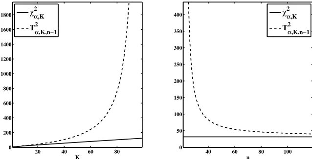
3.2 The critical values of theχ2_and_T2 _{tests versus the dimension}_K _and sample sizen . . . 34

3.3 Schematic representation of the observation vector, the weighting vec-tor and the projection vecvec-tor . . . 38

4.1 The power ofT2 and t∗ _{tests versus the sample size} _n _{. . . .} ₅₆

8.1 Power versus Mahalanobis distance ∆ for various tests . . . 122

8.2 Power versus the total sample sizenT for various tests . . . 123

8.3 RSSR versus Mahalanobis distance ∆ and the total sample size nT for various tests . . . 123

(12)

8.5 Power versus Mahalanobis distance for t+_AD test with various prior

estimates . . . 133

8.6 Power versus Mahalanobis distance for t+_AD test with various prior

estimates . . . 134

8.7 Power versus Mahalanobis distance for various single-stage tests . . . 135

8.8 Power versus Mahalanobis distance forz+ and z+_AD tests . . . 136

8.9 Power versus Mahalanobis distance for various GS and AD tests . . 137

8.10 Box-plots of the angle φ_t+

(13)

Acknowledgments

This thesis would not have come true without all those who have supported me in

many different ways over the last three and a half years.

First, I would like to thank my supervisors Professor John A.D. Aston and

Professor Nigel Stallard for the time and energy that they have spent with me these

years to provide guidance and support in so many different ways. I could not imagine

a better supervision. I would also like to thank Dr Fabio Rigat for the supervision

during the first period of my PhD, and Tom E. Nichols for providing the fMRI data

and his advice at various instances regarding fMRI applications.

Throughout these years I have had the opportunity to discuss my research

with various members of the department. I would like to thank the people of the

statistical inference and neuroimaging reading groups for many fruitful discussions.

Special thanks go to the members of my review panels, Dr Elke Thonnes, Dr Sach

Mukherjee and Professor Jane L. Hutton for providing useful feedback at various

instances during my PhD.

I also feel grateful to the Department of Statistics at the University of

War-wick for providing the facilities, the funding for attending various conferences, but

most importantly the stimulating environment for research. I would also like to

thank the Engineering and Physical Sciences Research Council that has funded my

studies through the Warwick Centre for Analytical Science (EP/F034210/1).

During my PhD I have had the chance to make some new friends that I would

like to thank for making my time more pleasant during these years. To name very

(14)

younger ones, Helen Ogden, Pantelis Samartsidis, Panayiota Touloupou, thank you.

I would also like to thank Chris for proofreading this thesis and Pantelis, Habib

Ganjgahi for helping me to produce an fMRI figure.

Lastly, I could not forget my friends, all my family members - my

grand-parents, my brothers-, sisters- and parents-in-law, my siblings, Giannis, Eleni and

her family, and my parents, Kostas and Loukia - and especially my wife Kyriaki for

(15)

Declarations

I hereby declare that this thesis is based on my own research, except when stated

otherwise, in accordance with the regulations of the University of Warwick, and has

not been submitted elsewhere.

The methodology in chapter 4 and part of the results in chapter 8 are

incor-porated in a paper [Minas et al., 2012] published in Statistics in Medicine (2012,

31) with the title: “A hybrid procedure for detecting Global Treatment Effects in

Multivariate Clinical Trials: Theory and Applications to fMRI Studies”. This is

joint work with F. Rigat, T.E. Nichols, J.A.D. Aston and N. Stallard.

The methods and results contained in chapters 6, 7 and 8 are joint work

with J.A.D. Aston and N. Stallard. The methodological part of this work is

sub-mitted for publication in a paper entitled: “Adaptive multivariate global testing”. A

draft of this paper [Minas et al., 2013] is published inCRISM research papers. The

application of this methodology to fMRI studies is incorporated in the conference

paper entitled: “ROI analysis of pharmafMRI data: an adaptive approach for global

testing” published in the “Proceedings of 46th Scientific meeting of the Italian

Sta-tistical Society, 2012”. T.E. Nichols also participated in this work. A paper that

considers wider application of this methodology to neuroimaging studies is to be

submitted for publication.

In all of these publications I have taken the leading role both in terms of

preparation of the material and conceptual work. In addition, all results presented in

(16)

In addition to the work presented in this thesis, a contribution to the

discus-sion of the paper: “Group sequential tests for delayed responses”, by L.V. Hampson

and C. Jennison, is published in theJournal of the Royal Statistical Society Series

(17)

Abstract

Global tests are a key research endpoint in multivariate studies. They provide an

omnibus assessment of the overall effects across the multivariate outcomes. This

global evaluation is clearly of high practical value in the field of neuroimaging,

which has become increasingly important in recent years. Existing global testing

methodologies, however, fail to accommodate the demands of neuroimaging studies

that have typically small sample sizes and highly correlated local outcomes.

In this thesis a novel class of multivariate global tests is developed. The

proposed tests are based on a formal framework for using prior information and

accumulated data to learn the effect direction. This framework is used to construct

test statistics that target the estimated effect direction, rather than the whole

multi-variate space, for detecting global effects. Adaptive designs are employed to allow for

sequential modifications of the test statistics, based on accumulated data, without

inflating the type I error.

A major focus in our methodology is power performance. The proposed tests

are shown to be optimal in terms of predictive power. Furthermore, a power

charac-terisation allowing us to explain the behaviour of our tests and perform simple power

analysis is derived. An extensive power analysis, including comparisons to

alterna-tive global tests, is performed. Applications to neuroimaging studies are illustrated

through two real examples. Our results show that the developed methodology can

be particularly useful in cases where the sample sizes are small and prior information

(18)

Abbreviations

MRI Magnetic Resonance Imaging

fMRI functional MRI

EEG Electroencephalography

MEG Magnetoencephalography

PET Positron Emission Tomography

BOLD Blood Oxygenation Level Dependent

CNS Central Nervous System

GLM General Linear Model

SPM Statistical Parametric Mapping

ROI Region(s) Of Interest

DFT Discrete Fourier Transformation

OLS Ordinary Least Squares

GLS Generalised Least Squares

SS Standardised Sum

PC Principal Component

SSD Single-Stage Design

GS Group Sequential (design or test)

GSD Group Sequential Design

AD Adaptive design (or test)

CIP Conditional Invariance Principle

CEF Conditional Error Function

(19)

Notation

The following notation is used throughout this thesis, unless otherwise stated. In

addition to their statement here, they are usually described at their first occurrence.

Unless otherwise stated, we use: (i) lower case, normal font type to represent scalars,

(ii) lower case,bold font type to represent vectors and (iii) upper case, bold font type for matrices. No distinction is made between random variables and observed

values in terms of notation, but, if not obvious by the context, this is made clear by

appropriate descriptions.

R the set of real numbers

RK the set ofK₋dimensional vectors with real entries

zT,AT transpose of a vector z, matrixA

c_K K₋dimensional vector with all entries equal to the scalarc

ang(a,b) angle, in measured degrees at the origin, between a and b

Diag(a1, a2, . . . , aK) K×K diagonal matrix with diagonal entries a1, a2, . . . , aK

Diag(a) diagonal matrix with diagonal the vector a

IK K×K identity matrix

E(_·) expectation function

P r(A) probability of eventA

(20)

N(µ, σ2) Normal distribution with mean µand variance σ

NK(µ,Σ) K−dimensional normal distribution with mean vectorµand

covariance matrixΣ

tν Student’st distribution withν degrees of freedom

tν(θ) Non-central t distribution with ν degrees of freedom and

location/non-centrality parameterθ

tK(ν,θ,S) K−dimensional non-centralt distribution withν degrees of

freedom, location/non-centrality parameterθand scale

ma-trixS

IWK×K ν,S−1

Inverse Wishart distribution with ν degrees of freedom and

scale matrixS

χ2_K χ2 distribution withK degrees of freedom

χ2

K(D) Non-central χ2 distribution with K degrees of freedom and

non-centrality parameterD

T2

K,n Hotelling’sT2 distribution with (K, n) degrees of freedom

T_K,n2 (D) Non-central Hotelling’s T2 distribution with (K, n) degrees

of freedom and non-centrality parameter D

φ(_·) The standard normal probability density function

Φ(_·) The standard normal cumulative density function

Ψθ,ν The cumulative distribution function of tν(θ)

ψθ,ν The probability density function oftν(θ)

∆ Mahalanobis distance

k dimension index

K dimension of observations

i subject index

n sample size

j stage index

(21)

H0 null hypothesis

H1 alternative hypothesis

α nominal type I error

β power

1₋β type II error

χ2 _test _{single stage multivariate}_χ2 _test

T2 _test _{single stage multivariate Hotelling’s}_T2 _test

χ2

GS test group sequential test with test statistic the multivariate χ2

T_GS2 test group sequential test with test statistic the multivariate

Hotelling’sT2 test

z test single stage test with test statistic the linear combination

z₋statistics with fixed weighting vector

t test single stage test with test statistic the linear combination

t₋statistics with fixed weighting vector

zGS test group sequential test with test statistics the linear

combina-tionz₋statistics with fixed weighting vectors

tGS test group sequential test with test statistics linear combination

z₋statistics with fixed weighting vectors

z+ test single stage linear combinationz₋test with weighting vector

selected using prior information and/or pilot data

t+ test single stage linear combinationt₋test with weighting vector

selected using prior information and/or pilot data

z_AD+ test adaptive linear combination z₋test with weighting vector

initially selected using prior information and sequentially

adapted to accumulating data at interim analyses

t+_AD test adaptive linear combination t₋test with weighting vector

initially selected using prior information and sequentially

(22)

Chapter 1

Introduction

Multiple outcomes emerge in almost every area of scientific investigation.

Natu-rally, when performing a scientific study, researchers wish to monitor a number of

measures for each experimental unit. With more measures recorded and explored,

one can develop greater knowledge about the problem. This multiplicity, however,

does not solely arise from scientific curiosity and luxury to collect more information,

but often because of the nature of the problem which implies that a single isolated

measure is not sufficient to answer key experimental questions. Particularly, in

med-ical studies, to evaluate the effects of a treatment on subjects, multiple symptoms

and bodily functions need to be monitored. This situation occurs in many other

fields of statistical application including industry, economics, ecology, biology and

psychology, in cases where multiple events or phenomena are essential to evaluate

an effect of interest.

A fundamental question arising in experimental studies, regardless of whether

single or multiple outcomes are evaluated, is whether the results provide significant

evidence for the existence of the effect of interest or not. This is most often a

key question. In the presence of multiple outcomes, it is translated as whether the

results provide significant evidence for an overall effect. An omnibus assessment

(23)

no treatment effect in any of the multiple outcomes is formed and suitable testing

procedures are constructed. These global tests, as opposed to being interested in

detecting “local” effects, as in effects on specific outcomes, simultaneously evaluate

multiple outcomes to provide a global statement for the presence of the treatment

effect.

Global testing is a classical field of statistical inference with several different

approaches being available. Multiple testing methods, such as Bonferroni correction,

can be used to evaluate global hypotheses. These are typically simple procedures,

usually constructed under weak modeling assumptions, but they become

conserva-tive if the multiple outcomes are highly correlated. In the latter case, it is often

useful to consider the multiple outcomes as multivariate observations and to

incor-porate correlations into the modeling assumptions. This multivariate approach is

especially appropriate when the multiple outcomes are biologically (or in some other

context) related. The classical multivariate global test, Hotelling’sT2, can efficiently

detect effects in every direction of the multivariate space, when the sample size of

the study, n, is sufficiently large. However, in settings where n approaches or

be-comes smaller than the observation dimensionK, theT2 _{test becomes respectively}

inefficient and inapplicable. This cost in efficiency, paid because of searching in

ev-ery direction of the alternative space, seems particularly wasteful if prior knowledge

about the direction of the effect is available.

The present thesis investigates global testing procedures in the presence of

multivariate observations. This work is motivated by an area which introduces new

challenges in global testing, highlighting some deficiencies of existing methodology

and necessitating the demand for novel methodology. This is the very exciting, and

rich in statistical applications, field of neuroimaging.

Neuroimaging uses powerful techniques, such as Magnetic Resonance

Imag-ing (MRI), to explore the anatomy, function and pharmacology of the normal and

(24)

of neural activity at various brain locations suggest a significant overall treatment

effect is fundamental. These local neural measures, even after substantial

sum-marisation, can have relatively large dimension. Furthermore, these measures are

typically highly correlated and the effects across them are often dispersed in the

sense that they are locally small, but, if combined, globally large. Another property

of neuroimaging studies is that the great amount of research in the area and the

spatial characterization of neural measures typically provide the researchers prior

information about various aspects of their investigation. Finally, the high cost of

neuroimaging equipment and expertise typically restricts sample size of

neuroimag-ing studies to small levels.

These properties are taken into consideration in the present thesis to develop

novel methodology for global testing. Multivariate assumptions are imposed on the

observation vectors enabling us to incorporate correlations and combine dispersed

local effects for a single global evaluation. The proposed tests are based on linear

combinations of the observation vectors. The crucial element in this approach is

the weighting vector reducing the observation vectors to scalar linear combinations.

This defines the direction in which we decide to search for effects, and it can

sub-stantially affect both type I and type II error rates of the tests. A formal framework

for selecting the weighting vector using prior information and pilot data without

inflating the type I error is developed. This enables the proposed tests to attain

high power levels for large sample sizes, but can be efficient even in situations where

the sample size is limited to relatively low values.

In a major development of our methodology, global testing procedures are

implemented within an adaptive design framework. Adaptive designs allow for

in-terim design modifications, based on the observed data, without inflating the type

I error rate. The use of adaptive design methodology increases the possible actions

of the proposed procedures and can potentially improve efficiency. The global test

(25)

based on accumulated data at subsequent interim analyses. Early termination of

the study, due to early acceptance or rejection of the null hypothesis at interim

analyses, is also possible within the adaptive design framework.

While the developed tests are analytically proved to control type I error, a

major focus of our methodology is power performance. The test statistics of the

constructed procedures are derived to be optimal, within the class of linear

com-bination tests, with respect to predictive power given the information available at

interim analyses. Furthermore, a framework for performing power analysis of

lin-ear combination tests is derived. In this, we reduce the complexities in performing

power analysis of linear combination tests, by re-expressing the possibly high

dimen-sional design space as a lower dimendimen-sional easily interpretable space, that is, still

sufficient to determine power. These results provide wide understanding of the

be-haviour of linear combination tests and allow us to perform relatively simple power

analysis. The main results of an extensive power analysis, including comparisons to

alternative tests and application to neuroimaging studies, is provided in this thesis.

Finally, it is useful to note here that the methodology developed in this thesis

is motivated by neuroimaging studies, but our framework is rather more generic

and can be applied for multivariate global testing in many other fields. Biomedical

studies and particularly clinical trials would likely provide an area of application.

Clinical trials are studies undertaken to examine the effects of different medical

interventions on human subjects [Friedman et al., 2010]. The issues of multiple

outcomes, global testing, error rates control are often crucial in clinical trials and

this is addressed by the present thesis.

1.1 Outline of the thesis

The remainder of this thesis is structured as follows.

(26)

intro-duced. I briefly summarize the current state of the field, focusing on the two

neu-roimaging modalities, functional MRI (fMRI) and Electroencephalography (EEG),

which I target in this work. fMRI and EEG data analysis is then discussed with

special attention given to the types of preparatory analysis that generated the two

datasets used throughout this thesis to illustrate applications of various global tests.

In chapter 3, we discuss the problem of testing global hypotheses. Various

global tests available in the literature are discussed, with special attention given

to their strengths and weaknesses. We first briefly discuss p₋value adjustment

methods, such as the Bonferroni global test. We then proceed to multivariate global

tests which are the broad focus of this thesis. We discuss the fully multivariateχ2

and Hotelling’s T2 tests and briefly introduce one-sided multivariate tests. Finally,

we proceed to the class of linear combination tests which is the specific area of

focus in this thesis. Here, we describe the available approaches in the literature

and address the weaknesses which we attempt to mitigate using the methodology

developed in later chapters.

In chapter 4, we develop novel methodology for performing linear

combi-nation tests. The class of linear combicombi-nation tests is first formally introduced.

Then, power-optimal linear combination tests are derived. Using this result, links

to O’Brien linear combination and Hotelling’s T2 _{test are derived. The}

power-optimal linear combination tests use weighting vectors which depend on unknown

model parameters. The weighting vectors which maximise predictive power given

prior information and preliminary data obtained from a pilot study are then derived.

The proposedz+ and t+ tests are discussed, while a comparison to the alternative

approach of a fully Bayesian test is also provided.

Adaptive designs provide the possibility of substantially improving the tests

developed in chapter 4. In chapter 5, the framework of adaptive design

methodol-ogy is introduced. Here sequential designs are also discussed as they are strongly

(27)

pro-vide the framework for various alternative global tests considered for comparison to

the developed methodology. The concepts that give rise to sequential and adaptive

designs are first discussed. Group sequential and adaptive testing is next developed

with the main attention given to the combination tests used in our methodology.

Finally, we briefly describe various types of applications of these designs available

in the literature, while the chapter is closed with a discussion for the current state,

challenges and potentials of the field.

In chapter 6, we develop a methodology for performing adaptive linear

com-bination tests. First, we formulate the J₋stage tests with stage-wise statistics

obtained via linear combinations. The power-optimal J₋stage linear combination

tests are then derived. The latter tests use weighting vectors which depend on

the unknown modelling parameters. For practical implementation, a framework for

sequentially updating the weighting vector, initially constructed based on prior

in-formation, using the data observed at interim analyses is constructed. Adaptation

rules maximising the predictive power given the interim results are derived. These

tests are analytically proved to control type I error.

The problem of performing power analysis of multivariate global tests and

particularly linear combination tests is discussed in chapter 7. We derive a power

characterisation of linear combination tests in terms of low-dimensional easily

inter-pretable parameter summaries. The implications of these results, with respect to

our understanding for linear combination tests and for performing power analysis,

are discussed.

In chapter 8, the main results of an extensive power analysis are presented.

We start by describing the effect of various design and model parameters on power

performance. Comparisons between various global tests, including the constructed

procedures, are next provided. Finally, application of various global tests on our

real examples of an fMRI and an EEG study are considered.

(28)

future developments and extensions of the proposed methodology.

(29)

Chapter 2

Neuroimaging studies

2.1 Introduction

In this chapter, we attempt to outline the enormously exciting field of neuroimaging

which has motivated the methodology developed in this thesis. Our target is to

establish our motivations and to provide the necessary background to understand

the examples to which we apply our methods.

We first briefly provide some background about neuroimaging and its current

state. We then provide some more details on the neuroimaging modalities, fMRI and

EEG, in which we are most interested. Here, we discuss fMRI and EEG data analysis

and particularly Regions of Interest (ROI) analysis of fMRI data and frequency

analysis of EEG data from which our real datasets are derived. We also introduce our

real examples arising from a fMRI drug development study and an EEG depression

study.

2.2 Neuroimaging

The study of the human brain has a long history tracing back at least to the father

(30)

in-different aspects of the nervous system. In the late 1960s, scientists of all these

disciplines decided to merge their knowledge under an interdisciplinary field coined

neuroscience. The Society of Neuroscience, formed in 1971, set a common principal

target for neuroscientists: to understand the structure and function of the normal

and abnormal brain. This initiated an era of revolutionary achievements and great

public interest with neuroscience being one of the leading areas of science today

and the Society of Neuroscience being, according to Bear et al. [2007], the “largest

and fastest-growing association of professional scientists in all experimental biology”

[Bear et al., 2007; Squire et al., 2008].

Neuroimaging is the branch of neuroscience that uses various techniques to

create images of the structure, function and/or pharmacology of the brain.

Struc-tural neuroimaging targets the description of brain anatomy, while functional

neu-roimaging attempts to describe the functional organization of the brain [Squire et al.,

2008]. Technological development enabled the invention of various neuroimaging

techniques over the 20th century [Raichle, 2000]. The consecutive discoveries of

Positron Emission Tomography (PET) in 1980s and especially fMRI [Ogawa et al.,

1992] in early 1990s led to an explosion of interest in functional neuroimaging over

the last decades (see for example Friston [2009]).

Neuroimaging is now the predominant technique in behavioral and

cogni-tive neuroscience [Cabeza et al., 2001; Friston, 2009] and it has a fast-growing role

in psychiatry [Phillips, 2012], evidence-based neurology [Burneo et al., 2011] and

image-guided neurosurgery [Aquilina et al., 2005]. An emerging application of

neu-roimaging is in the discovery and development of drugs for the treatment of disorders

of the Central Nervous System (CNS). This is regarded by many authors as a great

opportunity to respond to the increasing burden of CNS disorders by improving

the efficiency of current practice in CNS drug development [Matthews et al., 2011;

Wong et al., 2008].

(31)

acqui-sition. Using the various modalities of neuroimaging, the living human brain can be

studied with great spatio-temporal resolution while activated and possibly engaged

to symptom-related tasks. Many authors have argued that neuroimaging can play

an important role in early stages of drug development by providing objective

mark-ers of brain activity. Imaging biomarkmark-ers can replace subjective behavioral measures

especially to support proof-of-concept studies and go/no-go decision making. At the

current time, neuroimaging techniques are (strictly) not validated for drug

develop-ment, but most major pharmaceutical companies are embracing this technology by

establishing it in-house or via academic collaborations [Borsook et al., 2011; Wise

and Tracey, 2006].

Nevertheless, there are several challenges to be overcome before these

tech-niques become further established. The signal of various important neuroimaging

modalities needs to be better understood and neuroimaging traits of CNS diseases

need to be established. The high cost of the equipment and the need for trained

individuals to run the experiments most often limits the sample size of the studies,

while the pressure for efficiency remains high. Hence, there is a need for

standard-ized statistical methodologies specialstandard-ized to neuroimaging data analysis [Borsook

et al., 2011; Whitcher and Matthews, 2006]. We respond to the latter problems,

as we explain later, by providing methodology which uses the special properties of

neuroimaging to achieve high efficiency even in settings with small sample sizes.

The modalities of functional neuroimaging can be broadly separated into two

categories. The first, which mainly consists of Electroencephalography (EEG) and

Magnetoencephalography (MEG), directly measures brain activity by capturing the

electrical or magnetic signals produced by neurons during activation. The second,

which is currently dominated by functional Magnetic Resonance Imaging (fMRI)

and Positron Emission Tomography (PET), indirectly measures brain activity by

capturing changes in local blood flow linked with neuronal activation. The nature

(32)

which along with their invasiveness and their cost are important properties in terms

[image:32.595.126.536.201.423.2]

of application (see table 2.1).

Table 2.1: Properties of various neuroimaging modalities. Source: Lystad and Pol-lard [2009]

PET fMRI EEG MEG

Measure indirect indirect direct direct

Response haemodynamic haemodynamic neuroelectrical neuromagnetic

Invasive yes no no no

- confined yes yes no yes

- radiation yes none none none

Device cost $8,000,000 $2,000,000 $100,000 $2,000,000

Operating cost $1,500 $800 $150 $600

Temporal res 1-2 min 4-5 s <1 ms <1 ms

Spatial res 4 mm 2 mm 10 mm 5 mm

In the following, we discuss further two important neuroimaging techniques, fMRI

and EEG, which motivate the methodology developed in this thesis.

2.3 fMRI

The most prominent form of fMRI is based on the so-called Blood Oxygenation

Level Dependent (BOLD) contrast. BOLD fMRI (often simply called fMRI) uses

the strong magnetic fields generated by MRI scanners to capture the local changes

in blood oxygenation level that accompany neural activation. These local

haemo-dynamic responses of the brain are recorded in 3₋dimensional images with great

(33)

seconds) of the scanner is restricted by various issues including the delay of the

haemodynamic response to neural activation [Huettel et al., 2008].

Figure 2.1: Schematic representation of a subject in a fMRI scan. Image by Duff Hendrickson, U.W., Copyright Hunter Hoffman, U.W.

The key properties of fMRI are the non-invasive, unharmful nature of the

technique and the very high spatial resolution allowing for a study of the brain

at the systems level. fMRI is currently one of the main drivers in understanding

brain function. The potential of further application to drug development studies is

discussed in a number of review publications (see Iannetti and Wise [2007]; Matthews

et al. [2011]; Whitcher and Matthews [2006]; Wise and Tracey [2006] for overviews).

fMRI is currently used to study the function and pharmacology of the brain under

several pathologies, such as Alzheimer’s disease [Pihlajam¨aki and Sperling, 2008] and

drug addiction [Smith et al., 2010]). Honey and Bullmore [2004] report more than

50 published articles on psychopharmacological studies using fMRI while Schwarz

et al. [2011a,b] provide guidelines for good imaging practice in pharmacological fMRI

studies.

2.3.1 FMRI data analysis

The typical fMRI dataset produced by a single scanning session consists of BOLD

recordings acquired from a small number of subjects (often around 15) during a

relatively short period of time (few hundreds time points) at around 104 ₋₁₀5

voxels1 _{throughout the brain.}

(34)

The raw fMRI data is preprocessed using several techniques of signal

process-ing, image processing and statistics. This typically involves realignment and spatial

normalization using suitable transformations to register the raw data to a

com-mon reference image. Spatial smoothing and temporal filtering are also employed

to eliminate the most common experimental artifacts (such as motion and scanner

artifacts) and increase the signal-to-noise ratio [Poldrack et al., 2011]. The typical

approach to model the preprocessed fMRI data is to apply mass-univariate

Gen-eral Linear Models (GLMs) to the time-series of each voxel separately. Normality

is a common and generally acceptable assumption for the preprocessed fMRI data

[Friston et al., 2007; Lindquist, 2008; Poldrack et al., 2011]. The default approach

for statistical inference is based on maps of the brain, called Statistical Parametric

Maps (SPMs), depicting the value of thet-statistics for each voxel. Parametric (for

example random field theory) or non-parametric (for example permutation tests)

approaches are then widely used to handle the huge multiple-testing problem of

detecting activated voxels throughout the brain while controlling for false positives

[Friston et al., 2007; Poldrack et al., 2011].

The burden of this multiple-testing problem can be alleviated by restricting

the search for activated voxels only to specific brain areas. In the following, we

briefly describe one method of data reduction. This is the ROI analysis applied to

the fMRI study of the example in section 2.3.2.

ROI analysis

In fMRI data analysis, investigators often primarily target selected brain locations

called regions of interest (ROI). ROI analysis is also very often reported as

supple-mentary to the standard mass-univariate voxel-by-voxel analysis in fMRI studies.

Compared with the voxel-by-voxel approach, ROI analysis provides a number of key

benefits. First, in data exploration, it enables the investigator to take advantage of

(35)

regarding the anatomy and function of a great number of brain ROI. For similar

rea-sons, ROI analysis is more suitable than voxel-by-voxel analysis for studying specific

regional hypotheses about the drug action [Wise and Tracey, 2006]. Such

hypothe-ses are more strict and therefore potentially more conformable to the regulations of

drug authorities. Finally, ROI analysis results in a drastic reduction of data

dimen-sion and this is expected to substantially increase statistical power [Mitsis et al.,

2007; Poldrack et al., 2011].

The first step in ROI analysis is to define the exact location of the ROI

to be analyzed. This can be performed based on structural or functional features.

Structural or anatomical ROI can be defined based on anatomical landmarks of

the brain. These are described by standard brain atlases, such as the Talairach

atlas [Talairach and Tournoux, 1988], which are widely available. In some cases,

brain atlases can even be specific to the area of investigation. For example, Mitsis

et al. [2007] use a “pain-atlas” for a pain treatment study. Based on such atlases,

investigators define the detailed location of ROI in each subject either in terms of

the subject’s brain anatomy, derived using high-resolution structural MRI, or using

“probabilistic atlases” reflecting the anatomical variability between subjects. On

the other hand, functional ROI are often derived using an independent “localizer”

scan to identify voxels in particular brain areas that show a characteristic response

of interest. Finally, ROI can be defined based on previous studies, preferably from

a meta-analysis on the domain of interest. It is important to note that to control

the type I error, the ROI locations need to be defined prior to analyzing the data

of the main study [Poldrack et al., 2011].

The next step in ROI analysis is to quantify the measure to be extracted

from each ROI. One method is to count the activated voxels within the defined

ROI. However, this approach, used mainly in early fMRI studies, is very

sensi-tive to the specified activation threshold. More commonly, voxel-wise estimates, ˆβ,

(36)

mass-univariate GLM. These ˆβ-values are often standardized to the design of the

experiment by appropriate scaling. Summaries of the ˆβ-values across the voxels of

each ROI of each subject are then derived using either weighted (for example first

Principal Component [Friston et al., 2007]) or un-weighted averages. These averages

of the estimated effects constitute the ROI data which are used to derive statistical

inference for the brain action at, between or across the selected ROI [Poldrack et al.,

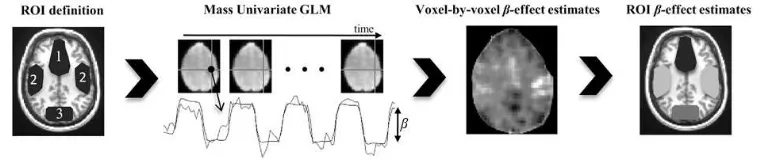
[image:36.595.130.510.276.356.2]

2011]. The main steps for deriving ROI data are also described in figure 2.2.

Figure 2.2: Typical steps of ROI analysis producing the multivariate outcome used in our real example in section 2.3.2. The preprocessed series of fMRI images are modelled at voxel-by-voxel resolution using mass univariate General Linear Models (GLMs). Suitable estimates of parameter values (β) expressing the treatment effect in each voxel are first extracted from the GLM and then averaged across the pre-defined ROI to produce a multivariate outcome where each component corresponds to a measure of the treatment effect in a specific ROI.

2.3.2 Example: fMRI drug development study

For the purposes of drug development, a fMRI study was conducted by

Glaxo-SmithKline plc. A total of 13 subjects participated in the study. At the planning

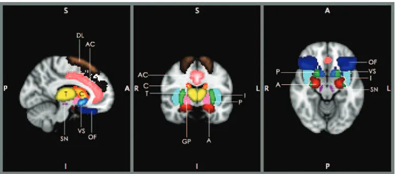
stage, the following anatomical ROI (see figure 2.3) were defined: 1. Anterior

Cin-gulate (AC), 2. Atlas Amygdala (A), 3. Caudate (C), 4. Dorsolateral Prefrontal

Cortex (DL), 5. Globus Pallidus (GP), 6. Insula (I), 7. Orbitofrontal cortex (OF),

8. Putamen (P), 9. Substantia Nigra (SN), 10. Thalamus (T), 11. Ventral Striatum

(VS).

ROI summary data was extracted from the mass-univariate GLM applied to

(37)

aver-aged across the voxels of each ROI for each subject. The available data represents

the difference between paired treatment-placebo observations across ROI for each

[image:37.595.128.515.176.346.2]

subject.

Figure 2.3: Approximate locations of ROI used in the fMRI study example. Each of the following ROI are indicated by a different colour and abbreviation: Anterior Cin-gulate (AC-pink), Atlas Amygdala (A-red), Caudate (C-red/yellow), Dorsolateral Prefrontal Cortex (DL-copper), Globus Pallidus (GP-magenta), Insula (I-purple), Orbitofrontal cortex (OF-blue), Putamen (P-green), Substantia Nigra (SN-cyan), Thalamus (T-yellow), Ventral Striatum (VS-blue/lightblue)

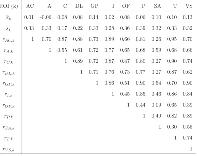
The means, standard deviations and correlations matrix of this ROI dataset

are presented in table 2.2. As we can see, effect sizes differ across ROI, the standard

deviations are relatively large and generally high correlations are observed.

Using this data, the investigators wished to address a fundamental question

arising in neuroimaging studies. This concerns the existence of global treatment

effects across ROI. The term global is used here to stress the difference to being

interested in local effects, as in effects at specific ROI. The null hypothesis to be

evaluated is then whether the treatment-placebo differences provide no statistically

significant evidence for treatment effects across the selected ROI. To answer this

global question, within this setting but also more generally, we employ various

test-ing procedures introduced in the next chapters. We now turn our interest to another

(38)

[image:38.595.125.518.145.457.2]

Table 2.2: Means, standard deviations and correlations of ROI data (nT = 13) of

the fMRI study.

ROI (k) AC A C DL GP I OF P SA T VS

¯

xk 0.01 -0.06 0.08 0.08 0.14 0.02 0.08 0.06 0.10 0.10 0.13

s_k 0.33 0.33 0.17 0.22 0.33 0.28 0.36 0.39 0.32 0.33 0.32

rAC,k 1 0.70 0.87 0.88 0.73 0.89 0.66 0.81 0.26 0.95 0.70

rA,k 1 0.55 0.61 0.72 0.77 0.65 0.68 0.59 0.68 0.66

rC,k 1 0.89 0.72 0.87 0.47 0.80 0.27 0.90 0.74

rDL,k 1 0.71 0.76 0.73 0.77 0.27 0.87 0.62

rGP,k 1 0.86 0.51 0.90 0.54 0.70 0.90

rI,k 1 0.45 0.85 0.46 0.86 0.84

rOF,k 1 0.44 0.09 0.65 0.39

rP,k 1 0.49 0.82 0.89

rSA,k 1 0.30 0.55

rT,k 1 0.74

rV S,k 1

2.4 EEG

EEG records the electrical activity of the brain. Specifically, EEG captures the

summed electrical potential generated by synchronously activated neurons (tens

of thousands). This activity is captured by electrodes typically placed at various

locations of the scalp. EEG has unrivalled temporal resolution (around 1-10

mil-liseconds) with recordings regarded as “real-time” measures. On the other hand,

spatial resolution has fundamental physical limits with up to a number of sites,

often called channels, sampled in routine studies. For clinical studies, typically 19

(39)

used [Gevins, 2002].

The high temporal resolution, the relatively low cost compared to other

neu-roimaging techniques, as well as the non-invasive, safe, portable equipment are the

main advantages of EEG. During the last decade, neuroscientists have shown great

interest in combining EEG with fMRI to achieve high spatial and temporal

resolu-tion [Mulert and Lemieux, 2010]. There is also interest in the so-called event-related

potentials (ERPs) which employ EEG to record brain response to specific stimuli

[Handy, 2005]. EEG has made great contribution in studying the effects and

phar-macology of various CNS-related disorders (see [Bauer and Bauer, 2005]),

particu-larly epilepsy [Thompson and Ebersole, 1999] and depression [Steiger and Kimura,

[image:39.595.252.391.368.526.2]

2010]. An example of the latter application is described in section 2.4.2.

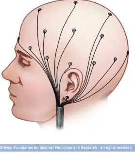
Figure 2.4: Schematic representation of the EEG electrodes placed on the scalp. Image source: www.riversideonline.com

2.4.1 EEG data analysis

EEG raw data of a single subject consists of multiple time-series recorded at a

num-ber of different location or channels. They are typically preprocessed by applying

high- and low-pass filters to eliminate experimental artifacts and possibly signals of

no interest for the study. Baseline correction is also applied by subtracting a “mean

(40)

artifacts such as sweating and muscle tension [Hauk, 2013; Sanei and Chambers,

2007].

EEG data can be analyzed as observed in the time-domain, but they are

of-ten transformed to the frequency-domain to perform data analysis. Frequency data

analysis is particularly important in EEG. The rhythms that characterize normal

and abnormal brain activity in EEG are categorized in four major frequency ranges.

These are (from low to high frequency): delta (0.5₋4 Hertz), theta (4₋8 Hertz),

alpha (8₋13 Hertz) and beta (13₋30 Hertz). In terms of cognition states, delta is

associated with deep sleep and theta with creative inspiration and deep meditation.

Alpha frequency is associated with relaxed awareness and beta is observed during

active thinking, focus and creation. Abnormal EEG signal in alpha and beta

fre-quency ranges is associated with various CNS related disorders (for example epilepsy

[Sanei and Chambers, 2007]).

The Discrete Fourier Transformation (DFT) is typically used to transform

the time-series of each channel to the frequency domain. Formally, the DFT is

defined as

y(f) =

N

X

t=1

x(t) exp−i2πf t,

where x(t) the response at time t and y(f) the amplitude of the spectrum at

fre-quency f. The square of the amplitude, (y(f))2, named the power spectrum, or

more commonly its logarithm, log y(f)2

, is then used in data analysis [Rao, 2010].

In practice, EEG data is typically segmented into short time intervals before

ap-plying the DFT. These epochs are defined by the clinicians, by taking into account

the experimental design, to ensure that they have similar characteristics. To avoid

discontinuities at the epoch edges, overlapping between them and suitable window

functions (such as the Hanning or Gaussian window) are often used. DFT is then

applied to the time-series of each epoch (after windowing and overlapping) to derive

(41)

data, the power spectra are typically averaged across these epochs to derive a

sum-mary aggregate power spectrum (stationarity assumptions are made here) for each

subject. This average power spectrum function, or the average power spectrum at

specific frequencies, are then often used for data analysis [Kropotov, 2009; Sanei

and Chambers, 2007]. Gaussianity is the typical assumption for the logarithms and

other transformations of the average power spectra [Collura et al., 2009; Lopes da

Silva, 2005; Sanei and Chambers, 2007].

2.4.2 Example: EEG depression study

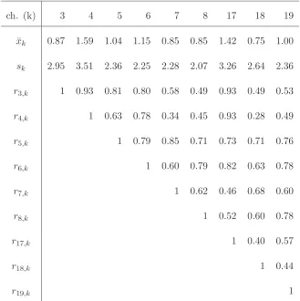
L¨auter et al. [1996] published frequency data from an EEG study. As they describe,

the data is collected fromn= 19 depressive patients at the beginning and at the end

of a six week therapy. The published data represent the changes on the absolute2

theta power of channels 3,4,5,6,7,8,17,19 (K = 9 locations, see figure 2.5) during

[image:41.595.259.373.423.549.2]

the therapy of each patient.

Figure 2.5: Schematic presentation of the position of the channels used in the EEG depression study

In table 2.3 we present the means, standard deviations and correlation matrix

of the data. Note that the correlations especially of nearby locations are high.

Furthermore, an increase in theta power is indicated in all channels, but the standard

deviations are generally high.

2_{The term absolute is used in EEG data analysis to distinguish from the relative power where,}

(42)

Similarly to the fMRI study in section 2.3.2, the investigators were

primar-ily interested in the global treatment effects. That is, they wished to investigate

whether the differences in the absolute theta power suggest a statistically

signifi-cant treatment effect across the selected channels. This question can be expressed

[image:42.595.156.485.258.588.2]

in terms of a global hypothesis.

Table 2.3: Means, standard deviations and correlations for the EEG depression study presented in L¨auter et al. [1996].

ch. (k) 3 4 5 6 7 8 17 18 19

¯

xk 0.87 1.59 1.04 1.15 0.85 0.85 1.42 0.75 1.00

sk 2.95 3.51 2.36 2.25 2.28 2.07 3.26 2.64 2.36

r3,k 1 0.93 0.81 0.80 0.58 0.49 0.93 0.49 0.53

r4,k 1 0.63 0.78 0.34 0.45 0.93 0.28 0.49

r5,k 1 0.79 0.85 0.71 0.73 0.71 0.76

r6,k 1 0.60 0.79 0.82 0.63 0.78

r7,k 1 0.62 0.46 0.68 0.60

r8,k 1 0.52 0.60 0.78

r17,k 1 0.40 0.57

r18,k 1 0.44

r19,k 1

2.5 Conclusions

Neuroimaging is a very important and exciting field of neuroscience. Neuroimaging

studies can provide great insight into the normal and abnormal brain anatomy and

(43)

clinical trials setting, a number of challenges remain outstanding and some of them

regard statistical methodology.

Some of these challenges are illustrated by the real examples of the fMRI and

EEG study. These studies share common properties which are typical in

neuroimag-ing studies. Firstly, high correlations are observed especially but not exclusively

be-tween nearby locations. Secondly, the observed effects are dispersed across different

locations, in the sense that they are locally small but, as we show in section 3.3.1,

globally large. This suggests combining the local outcomes, rather than treating

them separately, to detect global effects. In addition, due to the high cost of these

studies, the sample size is small and even after the reduction in data dimensionality

(for example using ROI or frequency analysis) remains close to the observations’

dimension. Furthermore, for these studies but also more generally in neuroimaging,

there are opportunities to elicit prior information from earlier results. In section

8.4 we provide some examples of such prior information which may arise from the

spatial characterization of the signal and from the nature of the study. Lastly, as

our examples illustrate, effects are often expressed in different directions between

brain locations with hyperactivation simultaneously occurring with deactivation.

These properties of neuroimaging studies are taken into consideration in the

methods introduced in later chapters. The deficiencies of existing global tests in

(44)

Chapter 3

Global testing

3.1 Introduction

As we discussed in the previous chapter, in neuroimaging studies the neural

ac-tivity is simultaneously investigated at multiple brain locations. More generally,

in biomedical studies but also in experiments performed in many other fields (for

example industry, ecology and psychology), investigators are often interested in a

number of outcomes and only rarely focus on a single measure. This situation often

becomes necessary due to the nature of the research questions. For example, in order

to evaluate the treatment effect on patients, multiple symptoms and relevant body

functions need to be monitored and hence multiple outcomes need to be evaluated

[D’Agostino and Russell, 2005; Dmitrienko et al., 2010].

In this chapter, we consider methods that can be used to evaluate

treat-ment effects in settings where multiple outcomes are studied. Specifically, we are

interested in testing procedures which can be used to evaluate global effects

ob-served across these outcomes. That is, as opposed to focusing on local effects on

specific outcomes, we consider methodology which evaluates multiple outcomes

si-multaneously to provide an omnibus assessment of the effects over all the outcomes.

(45)

observed outcomes suggest a significant treatment effect. [D’Agostino and Russell,

2005; O’Brien, 1984; Pocock, 1997; Sankoh et al., 1997]. This methodology can be

used to evaluate the question posed by the examples of neuroimaging studies, as

seen in sections 2.3.2 and 2.4.2, regarding global treatment effects across multiple

brain locations.

In the following, we consider various testing procedures, focusing mainly on

the essence of their methodology and discussing when they are appropriate. We

discussp₋value adjustment methods and multivariate tests, including “fully”

mul-tivariate tests and the class of linear combination tests which is the main

method-ological focus in this thesis. We begin with a general formulation of the global

testing problem.

Formulation

The K₋dimensional observation vectors, xi = (xi1, xi2, . . . , xiK)T, of subjects i =

1,2, . . . , n, are assumed to be independent with common mean vector E(x) =

µ = (µ1, . . . , µK)T and covariance matrix (the symmetric positive definite) Σ =

(σkk′)K_k,k′₌₁. The mean vector µ is often interpreted as the effect of interest or the

treatment effect. We wish to test the global null hypothesis of no treatment effect

against the two-sided alternative. That is,

H0 :µ=0K = (0,0, . . . ,0)T versus H1 :µ6=0K. (3.1)

In global testing, and more generally in statistical hypothesis testing, we are

inter-ested in controlling or minimising the potential incorrect decisions, called errors, of

the test. Specifically, we focus on controlling the type I error rate as in ensuring

that

(46)

and minimising the type II error rate

1₋β =P r( not reject H0 |µ=µ1), (µ1 6=0K) (3.3)

or, equivalently, maximising the power of the test

β=P r( reject H0|µ=µ1). (3.4)

If the type I error is equal to the significance level α, that is, the equality in (3.2)

is satisfied, we say that the test controls/maintains the type I error exactly or,

simply, the test is exact. The target of maximising power is sometimes replaced by

minimising the sample size of the test (or other design parameters) while controlling

power at a fixed level. We stress that in this thesis power is denoted by the letter β

rather than the (more common) expression 1₋β, to simplify notation.

Note that the testing procedures which follow equally apply to the

two-sample setting with common covariance matrix. This can be formulated in terms

of two independent samples, xAi, xBi, i = 1,2, . . . , n from groups A and B, with

E(xAi) = µA, E(xBi) = µB, var(xAi) = var(xBi) = Σ which are used to test

the null hypothesis H0 : µA−µB = 0K against the two-sided alternative H0 :

µA−µB6=0K. Furthermore, the setting of paired multivariate observations (as in

observations before and after a treatment), where the multivariate outcomes are set

equal tod_i =x_Ai₋x_Bi,i= 1,2, . . . , n, can also be accommodated by the methods

which follow. Finally, with a few trivial changes in the procedures to follow, the

situation where the hypotheses of interest are H′

0 :µ=µ0 and H1′ :µ6=µ0, with

µ0 6= 0K can also be accommodated. However, to simplify notation we continue

(47)

3.2 P

₋

_{value adjustment methods}

The above global hypotheses can be evaluated usingp₋value adjustment methods,

such as the Bonferroni test. In the well-known Bonferroni correction test, the local

outcomes, x1, x2, . . . , xK, are used to construct the statistics t1, t2, . . . , tK, with

correspondingp₋valuesp1, p2, . . . , pK, to test the local null hypotheses

H0k : µk= 0, k= 1,2, . . . , K.

The Bonferroni test rejects the k₋th local null hypothesis H0k if and only if pk ≤

α/K. Note that the global null hypothesis H0 in (3.1) can be written as the

inter-section of the local null hypotheses, formally

H0 =

K

\

k=1

H0k, (3.5)

and thus rejection of a local null hypothesis implies rejection of the global null

hypothesis.

Thus, by ordering thep₋values as p₍₁₎_≤p₍₂₎_{≤ · · · ≤}p₍_K₎, we can write the

global Bonferroni test as

reject H0 iff p(1) ≤α/K. (3.6)

Due to the first-order Bonferroni inequality (Boole’s inequality) this procedure

con-trols the type I error at the nominalα level [D’Agostino and Russell, 2005].

The global Bonferroni test is easy and convenient to apply and it does not

require any distributional assumption to control the type I error. It can even be

used if the observations of each dimension are measured at a different scale. On

the other hand, the Bonferroni method relies entirely on the smallest p₋value and

(48)

nominalα level) and inefficient (that is, power at unexpectedly low levels). This is

the case when, as in our motivating example, high correlations exist between the

local outcomes. The problem becomes worse as the dimension,K, of the observation

vectors increases. Pocock et al. [1987] and Dmitrienko et al. [2010] found, through

simulation studies, that for large positive correlations, especially when these are

higher than 0.5, the type I error rate of the Bonferroni method is substantially

lower than the nominal level. The results in Dmitrienko et al. [2010] show that the

conservatism is considerably larger if the observation dimension is increased even

from K = 2 to K = 5. We next consider the application of the global Bonferroni

test to the examples in sections 2.3.2 and 2.4.2.

Example: Global Bonferroni test for fMRI and EEG study data

We compute the values of the t test statistics and the corresponding two-sided

p₋values (12 degrees of freedom) at each of the 11 ROI.

Table 3.1: The local t₋ and p₋values for the observations collected at each ROI used in the fMRI study.

ROI AC A C DL GP I OFC P SA T VS

tk 0.03 -0.72 1.80 1.28 1.55 0.21 0.76 0.59 1.14 1.10 1.46

pk 0.98 0.48 0.10 0.23 0.15 0.84 0.46 0.57 0.28 0.29 0.17

The smallest p₋value p₍₁₎ = p3 = 0.10 is clearly larger than α/K ≈ 0.0045 for

α= 0.05,K = 11 and thus the Bonferroni method fails to reject H0.

Similarly, in the next table, we present the t₋ and p₋values of the theta

(49)

Table 3.2: The localt₋and p₋values for the observations collected at each channel used in the EEG depression study.

ch. 3 4 5 6 7 8 17 18 19

tk 1.29 1.97 1.92 2.22 1.63 1.80 1.90 1.24 1.84

pk 0.22 0.06 0.07 0.04 0.12 0.09 0.07 0.23 0.08

The smallestp₋value is p₍₁₎ =p4 = 0.04> α/K ∼= 0.0055 forα = 0.05,K = 9 and

thus the Bonferroni method fails to rejectH0.

A number of modifications of the Bonferroni method exist in the literature.

Simes [1986] global test rejects H0 if and only if p(k) ≤ kα/K, for at least one k,

k= 1,2, . . . , K. This test does not rely heavily on the smallestp₋value and it is less

conservative and more efficient than the Bonferroni method. Further, despite the

slight increase in computation, it is still very easy and convenient to apply. However,

Simes’ global test does not always control the type I error. Simes [1986] analytically

proved that his test controls type I error for independent outcomes, while, through

simulations, he showed that the type I error is also controlled for specific correlation

structures under various distributions including the multivariate normal. Hommel

[1988] also proposed two p₋value adjustment methods, which control the type I

error and are less conservative than Bonferroni method but more conservative than

Simes global test [D’Agostino and Russell, 2005].

The above methods completely ignore correlations and thus they all become

conservative when correlations are high. Some p₋value adjustment methods

ac-counting for correlations exist in the literature (for example James [1991], random

field theory [Friston et al., 2007] and non-parametric [Westfall and Young, 1993]

methods), but these tend to require complex calculations and they often rely on

Multivariate global testing and adaptive designs

University of Warwick institutional repository: http://go.warwick.ac.uk/wrap

A Thesis Submitted for the Degree of PhD at the University of Warwick

http://go.warwick.ac.uk/wrap/58321

This thesis is made available online and is protected by original copyright.

Please scroll down to view the document itself.

Library Declaration and Deposit Agreement

Giorgos Minas

0852199

5

Multivariate Global Testing and Adaptive Designs

Giorgos Minas

Department of Statistics

Contents

List of Tables

List of Figures

Acknowledgments

Declarations

Abstract

Abbreviations

Notation

Chapter 1

Introduction

1.1

Outline of the thesis

Chapter 2

Neuroimaging studies

2.1

Introduction

2.2

Neuroimaging

2.3

fMRI

2.4

EEG

2.5

Conclusions

Chapter 3

Global testing

3.1

Introduction

3.2

P

−

value adjustment methods

₋

_{value adjustment methods}